Talbot effect in cylindrical waveguides

Abstract

We extend the theory of Talbot revivals for planar or rectangular geometry to the case of cylindrical waveguides. We derive a list of conditions that are necessary to obtain revivals in cylindrical waveguides. A phase space approach based on the Wigner and the Kirkwood-Rihaczek functions provides a pictorial representation of TM modes interference associated with the Talbot effect.

1 Introduction

Although the Talbot effect was discovered firstly in the beginning of nineteen century (1836) and then rediscovered many times in different systems, it has never been a widely known phenomenon. In quantum systems it is often referred as “self-imaging” or “quantum revivals”. Even in the optical domain not always Talbot name is mentioned when this phenomenon is described and discussed. However, it was W. H. F. Talbot, who firstly observed that monochromatic light passing through periodic grating at a certain distance from the grating forms its ideal image and consecutively at integer multiples of this distance similar images are reproduced. He also demonstrated that when white light is used, images of the grating of different colors are formed at different distances and that is why we believe that all “self-imaging” effects should be referred as Talbot effects.

After the original paper by Talbot [1], followed by the work of Lord Rayleigh [2], and then by a series of papers of Wolfke [3], many papers have been written about this subject. A comprehensive description of the Talbot effect and its rediscoveries in classical optics can be found in Patorski [4]. Similar historical review and a detailed description of “quantum revivals” can be found in [5]. In the last years of the XX century fractional aspects of the Talbot effect attracted considerable interest [6, 7, 8, 9]. These effects were studied both in optical and quantum mechanical domains. As regards Talbot effect in optical waveguides most significant are works of Ulrich [11], who investigated waveguides of planar and ribbon geometries.

The literature concerning the Talbot effect in planar or rectangular waveguide geometries is quite reach (even some US patents for applications of the Talbot effect in those systems exist), but the much more practical cylindrical geometry was not taken into account in optical studies. We present in this paper a comprehensive theoretical study of the Talbot effect in cylindrical waveguides. This should fill the gap in the available descriptions of self-imagining phenomena in various waveguides. There is a limited number of papers mentioning cylindrical geometry in quantum revivals [12], but the results presented in this paper go beyond the one obtained so far.

The paper is organized as follows. In Section 2 we present general assumptions from which our study starts. We use a formal similarity between field propagation in waveguides and the dynamics of wave packets in potential wells in a given geometry. Using this analogy phase space Wigner and Kirkwood-Rihaczek functions are used. The phase space functions provide a pictorial description of interference effects, that are the basis of the Talbot revivals. In Section 3, the case of dielectric fibers and the possibility of revivals in this most practical for possible application system is studied. In Section 4, solutions of the wave equation in cylindrical mirror waveguides are analyzed and requirements that have to be fulfilled to obtain revivals are derived and imposed. A detailed study of approximations used is included. Finally, a summary of the results is given with a short paragraph devoted to the presentation of the applied method.

2 Talbot effect in phase space

2.1 General assumptions

The reason why the Talbot effect appears both in optical and quantum mechanical systems, mathematically can be summarized very briefly: The Helmholtz equation is common for classical electrodynamics and quantum mechanics. The dependence of the electromagnetic field in the direction of field propagation can be regarded as an analogue of time dependence of a wave packet in quantum mechanics. In the regime where paraxial approximation is justified this analogy is especially clear.

This paper is focused on Talbot revivals of an initial field in cylindrical waveguides which is purely an optical phenomenon but, nevertheless, as we shall see in the next paragraphs, its most simple explanation can be given referring to quantum mechanical concept of phase space distributions. The key question we shall pose and answer is whether the Talbot effect in cylindrical waveguides exists and can be used in practice.

We assume that harmonic, monochromatic plane waves propagate through the waveguide which symmetry axis was chosen as the $z$ direction of the system. Inserting the fields

$${\mathbf{E}}(x,y,z,t)={\text{E}}(x,y)e^{\pm ikz-i\omega t},\qquad{\mathbf{B}}(x,y,z,t)={\text{B}}(x,y)e^{\pm ikz-i\omega t}\,,$$ (1)

into the Maxwell equations, we obtain the two-dimensional Helmholtz equation:

$$\big{[}\nabla^{2}_{\perp}+\gamma^{2}\big{]}\left(\begin{array}[]{c}{\text{E}}\\ {\text{B}}\end{array}\right)=0\,,\quad{\text{where}}\quad\gamma^{2}=\mu\varepsilon\frac{\omega^{2}}{c^{2}}-k^{2}\,,\quad\nabla^{2}_{\perp}=\nabla^{2}-\frac{\partial^{2}}{\partial z^{2}}\,.$$

The propagating constants $k_{i}$ corresponding to specific modes are to be derived from appropriate boundary conditions (see, e.g. [13]).

2.2 Phase space distributions

As we have already mentioned the basis of Talbot effect, i.e. interference, is especially clearly seen in the phase space description. The quasi–distribution functions used for the study of electromagnetic fields, especially pulses, usually work in the time–frequency domain. Here, a totally different approach was chosen as all the fields taken into consideration are assumed to be monochromatic and of a harmonic time–dependence. Thus, we shall use a typical phase space known from mechanics constructed from the position and momentum variables.

Some complications result from the fact that the electromagnetic field requires a vector description. However, in many cases (e.g. mirror waveguides) solutions of the Maxwell equations are divided into $TM$ and $TE$ modes, i.e. are of type entirely determined by the $E_{z}$ or $B_{z}$ field component, respectively. Thus, we can treat $E_{z}$ ($B_{z}$) component, that fully describes the field, as a single scalar function corresponding to the quantum mechanical wave function of a potential well problem with analogous geometry.

To present problems of revivals is phase space we shall use the following two quasi-distribution functions: the Wigner function [14, 15],

$$W_{\Psi}(\vec{x},\vec{p})=\frac{1}{(2\pi)^{\mathrm{d}}}\;\int\Psi^{\star}(\vec{x}+\vec{\xi}/2)\;e^{{i\vec{p}\vec{\xi}}}\,\Psi(\vec{x}-\vec{\xi}/2)\,d_{\mathrm{d}}\xi\;,$$ (2)

which is the most commonly known phase space distribution, and the Kirkwood-Rihaczek (K-R) function [16, 17]:

$$K(\vec{x},\vec{p})=\frac{1}{(2\pi)^{\mathrm{d}}}\int d_{\mathrm{d}}\xi\,\Psi^{\star}(\vec{\xi})\,e^{{i(\vec{\xi}-\vec{x})\vec{p}}}\,\Psi(\vec{x}).$$ (3)

that is very convenient for calculations. Subscript $\mathrm{d}$ in the definitions above denotes number of spatial dimensions of the system, whereas $\Psi$ is a function that characterizes a system (e.g. wave function in quantum mechanical applications, or $E_{z}$ field component for TM modes in waveguides, etc.) Because for 3 dimensional systems phase space distributions are 6 dimensional, graphically only selected cross-sections can be presented. This arbitrary choice is made somehow easier for solutions of the form of Eq. (1), when the $z$-dependence of the field separates from the transversal components. Figure 1 shows examples of the “transversal” Wigner and K–R functions calculated for $E_{z}=J_{0}(j_{1}r)-J_{0}(j_{2}r)$, which corresponds to superposition of TM₀₁ and TM₀₂ modes in cylindrical mirror waveguide: $j_{1}$, $j_{2}$ denote the first and the second zero of Bessel function $J_{0}(u)$ and $r=\sqrt{\frac{x^{2}+y^{2}}{a^{2}}}$, where $a$ is a waveguide radius.

      

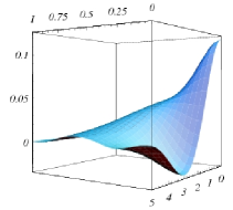
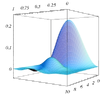
Figure 1: The $y=0$ and $p_{y}=0$ cross-sections of “transversal” quasi–distributions corresponding to $E_{z}=J_{0}(j_{1}r)-J_{0}(j_{2}r)$: a) cross-section of the Wigner function; b) cross-section of the real part of the K-R function.

As we have already mentioned in the case of solutions of Maxwell equations having the plane wave form we consider here, the $z$-dependence of the field separates from the transversal components. Thus, when describing Talbot effect, we can simply “forget” the transversal dependence of the field and concentrate on the $z$–$p_{z}$ cross-section of the phase space distribution which is essential for the Talbot revivals. Integrals corresponding to the $\exp(-ik_{i}z)$ factors are quite elementary and the cross-sections of quasi-distribution functions for given $x$, $y$, $p_{x}$, $p_{y}$, i.e. set the transversal position and momentum components, are easy to obtain.

The Wigner function for a superposition of two plane waves $\exp(-ik_{1}z)+\exp(-ik_{2}z)$ is given by

$$W_{\mathbf{2}}(z,p_{z})\sim\delta(p_{z}-k_{1})+\delta(p_{z}-k_{2})+2\,\delta\left(p_{z}-\frac{k_{1}+k_{2}}{2}\right)\cos(z(k_{2}-k_{1})).$$ (4)

The real part of the K–R distribution for such a superposition takes the form

$$\!\!\mathrm{Re}[K_{\mathbf{2}}(z,p_{z})]\!\sim\delta(p_{z}\!-\!k_{1})\!+\!\delta(p_{z}\!-\!k_{2})\!+\!\left[\delta(p_{z}\!-\!k_{1})\!+\!\delta(p_{z}\!-\!k_{2})\right]\cos[z(k_{2}\!-\!k_{1})].$$ (5)

When there are $N$ superposed waves, the following sums are obtained:

$$W_{N}(z,p_{z})\sim\sum_{i=1}\delta(p_{z}-k_{i})+2\sum_{1=i<j=N}\delta\bigg{(}p_{z}-\frac{k_{i}+k_{j}}{2}\bigg{)}\cos[z(k_{i}-k_{j})]$$ (6)

for the Wigner function and, for the real part of the K–R function,

$$\mathrm{Re}[K_{N}(z,p_{z})]\sim\sum_{j=1}^{N}\delta\left(p_{z}-k_{j}\right)\bigg{(}1+\sum_{i=1,\,i\neq j}^{N}\cos\left[z(k_{i}-k_{j})\right]\,\bigg{)},$$ (7)

with appropriate coefficients. In both cases the whole $z$ dependence is inserted into interference $\cos[z(k_{i}-k_{j})]$ terms. Initially, at $z=0$, all this cosines are equal to 1. The further $z$ dependence is guided by $(k_{i}-k_{j})$ factors. When all these $(k_{i}-k_{j})$ factors are commensurable with each other, perfect regular revivals are obtained at such $z_{rev}$ for which all $\cos[z_{rev}(k_{i}-k_{j})]$ are simultaneously equal to 1 again.

Obviously, all superpositions of just two different modes, like Eqs. (4), (5), will revive perfectly at multiples of $\frac{2\pi}{k_{2}-k_{1}}$, no matter what kind of waveguide we consider. But, when there is more superposed modes, commensurability of all possible $(k_{i}-k_{j})$ factors is needed to obtain perfect revivals. As the propagating constants $k_{i}$ vividly depend on the type of waveguide and its parameters, such a commensurability is rather an exceptional then a typical case. Even dealing with highly symmetric problems like mirror waveguides of planar or square cross-sections we have to keep in mind that $k_{i}=\sqrt{k_{0}^{2}-\gamma_{i}^{2}}$ which means that commensurability of $\gamma_{i}$’s (in these waveguides $\gamma_{i}$’s are commensurable) is not automatically followed by commensurability of propagating constants $k_{i}$. Only when linear approximation of $\sqrt{k_{0}^{2}-\gamma_{i}^{2}}$ holds, commensurability of $\gamma_{i}$’s is sufficient and that is why we shall often limit ourselves to the lowest from propagating modes. A definite advantage of working within the range where the linear approximation of square root holds for systems having $\gamma_{i}$’s proportional to each other is the fact that for a given wavelength the Talbot distance is settled, it does not depend on superposed modes. Otherwise, different modes superpositions shall revive at different distances.

All the features characteristic for the Talbot effect can be clearly explained by looking at interference $\cos[z(k_{i}-k_{j})]$ terms, their getting in and out of phase. The phase space description brings us in a natural way to this simple idea and indicates how fundamental this concept is.

3 Talbot effect in dielectric waveguides

Cylindrical dielectric waveguides are called optical fibers. We shall analyze only the step–index fibers, i.e. the fibers with constant refractive indexes in the core and the cladding, which are entirely characterized by radii of core and cladding and their reflective indexes $n_{1}=\sqrt{\mu_{1}\varepsilon_{1}}$ and $n_{2}=\sqrt{\mu_{2}\varepsilon_{2}}$. Assuming that the cladding and the core differ only by dielectric constants (magnetic permeabilities $\mu_{1}=\mu_{2}$) the standard boundary conditions lead to the following equation [18, 19]

$$\left[\frac{1}{\Gamma}\frac{J^{\prime}_{\nu}(\Gamma)}{J_{\nu}(\Gamma)}+\frac{1}{\kappa}\frac{K^{\prime}_{\nu}({\kappa})}{K_{\nu}({\kappa})}\right]\left[\frac{n_{1}^{2}}{\Gamma}\frac{J^{\prime}_{\nu}(\Gamma)}{J_{\nu}(\Gamma)}+\frac{n_{2}^{2}}{\kappa}\frac{K^{\prime}_{\nu}({\kappa})}{K_{\nu}({\kappa})}\right]=\frac{\nu^{2}\omega^{2}}{k^{2}c^{2}}\left[\frac{n_{1}^{2}}{\Gamma^{2}}+\frac{n_{2}^{2}}{{\kappa}^{2}}\right]^{2}\,,$$ (8)

where $a$ denotes the core radius, $\,\,\Gamma=a\gamma\,$, $\,{\kappa}=a\beta\,$, $\,\gamma^{2}=\mu_{1}\varepsilon_{1}\frac{\omega^{2}}{c^{2}}-k^{2}\,$ and $\beta^{2}=k^{2}-\mu_{2}\varepsilon_{2}\frac{\omega^{2}}{c^{2}}$. Although Eq. (8) has a quite nice regular form there is no way to solve it analytically. In the simplest case when the field has no azimuthal dependence, i.e. $\nu=0$, its solutions can be divided into $TE$ and $TM$ type, as for the mirror waveguides. Then a graphical picture gives a clear representation of solutions similarly to the case of finite potential wells in quantum mechanics. However, we have to keep in mind that the $\varphi-$independence, corresponding to $\nu=0$, is not a typical case. General solutions of Eq. (8) are $\varphi$ dependent and, actually, the lowest propagating mode in step-index dielectric fiber is obtained for $\nu=1$. Thus, let us start our analysis from general solutions.

3.1 General solutions in step index fibers

The lowest propagating mode in a cylindrical dielectric waveguide is always an $HE_{11}$ mode (in this notation $HE$ means that field $H_{z}$ dominates over $E_{z}$ field, while for $EH$ modes the $E_{z}$ field dominates). Single mode fibers are of a great practical importance, but in this study we are not interested in them because a single mode propagates without a change in its transverse distribution. Next modes are $TE_{01}$, $TM_{01}$, and $HE_{21}$. They appear almost simultaneously as their propagating constants are nearly the same.

Let us firstly consider a fiber in which there are only these four propagating modes (e.g. $\lambda=1550nm$, $n_{1}=1.46$, $n_{2}=1.45$, $a=4.5\mu m$). We shall refer to this situation as to the “limit of small number of modes”. Numerical solutions of Eq. (8) obtained for these parameters are: $a\gamma_{HE_{11}}=1.79268$, $a\gamma_{TE_{01}}=2.75973$, $a\gamma_{TM_{01}}=2.76234$, $a\gamma_{HE_{21}}=2.76342$. While analyzing problem of revivals of superpositions of $HE_{11}$, $TE_{01}$, $TM_{01}$, and $HE_{21}$ modes, one has to realize that although four modes are superposed, it is a special case when three propagating constants (corresponding to $TE_{01}$, $TM_{01}$, and $HE_{21}$ modes) are really close to each other. As we have already mentioned, superpositions of arbitrary two modes with propagating constants $k_{1}$, $k_{2}$ shall revive at all integer multiples of $z_{T}=\frac{2\pi}{k_{1}-k_{2}}$. It is easy to calculate that initial images constructed from superposition of pairs ($HE_{11}$, $TyE_{01}$), or ($HE_{11}$, $TM_{01}$) or ($HE_{11}$, $HE_{21}$) shall revive at multiples of $z^{t}_{1}=3,40787mm$, $z^{t}_{2}=3.3967mm$, $z^{t}_{3}=3.39214mm$, respectively. Those values are so close to each other that images constructed from all four modes shall revive at a mean value which is $\bar{z}_{T}=3.39891mm$. In numerical simulations of field propagation one can observe the first, second and even 20th or 50th Talbot revival. Obviously, higher revivals are less accurate, and after several tenths of faithful revivals they get out of phase – but then, after some propagating distance they get in phase again, and again some faithful revivals are obtained. Then the situations of getting in and out of phase appropriate cosines repeats almost cyclicly.

Plots of initial light intensity corresponding to superposition of $TM_{01}-TE_{01}-HE_{11}-2HE_{21}$ modes, its first Talbot revival and a characteristic inverted image at the half of the Talbot distance are presented in Figure 2. Infidelities of subsequent revivals, can be calculated using standard measure

$$f_{0}(z)=\frac{\|I(0)-I(z)\|}{\|I(0)\|}=\left(\frac{\int_{0}^{2\pi}d\varphi\int_{0}^{1}d\rho\,\rho\,|I(\rho,\varphi;0)-{I}(\rho,\varphi;z)|^{2}}{\int_{0}^{2\pi}d\varphi\int_{0}^{1}d\rho\,\rho\,|I(\rho,\varphi;0)|^{2}}\right)^{\frac{1}{2}},$$ (9)

to which we refer as to the infidelity as its value increases with increasing deviation of $I(z)$ from original $I(0)$ and only when $f_{0}=0$ the copy is perfect. For superposition of $HE_{11}-TE_{01}-TM_{01}-2HE_{21}$ modes the infidelities of the successive revivals are quite low ($f_{0}=0.0000276$, $f_{0}=0.0029825$, $f_{0}=0.0260536$, $f_{0}=0.0945819$ correspond to the 1st, 10th, 30th, and 60th revival, respectively) and in such a four-mode fiber infidelities of revivals for every initial field distribution would be of this order.

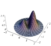
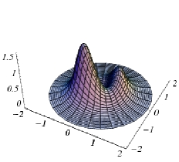
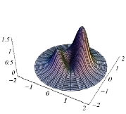
Figure 2: Superposition of $TM_{01}-TE_{01}-HE_{11}-2HE_{21}$ modes:  a) the original intensity; b) intensity at the half of the Talbot distance; c) 1st Talbot revival.

It is seen that in the limit of small number of modes Talbot revivals in dielectric fibers can be obtained. Change of fibers parameters will result in the change of Talbot distance, but it is quite obvious that for a small number of propagating modes Talbot revivals can be obtained. Just as we have seen using phase space representation – appropriate number of cosines have to get in phase to obtain the revivals.

This simple and quite intuitive method of looking for the Talbot distance starts to be more complicated when the number of propagating modes increases. Then, different methods are have to be applied to calculate revival distance as we shall see in the next section on the example of $TE_{0i}$ modes.

3.2 The $\varphi$–independent case ($\nu=0$)

The $\varphi$–independent solutions of Eq. (8) can be divided into $TE$ and $TM$ modes. For $TE$ modes the following relation is obtained:

$$\frac{1}{\Gamma}\frac{J_{1}(\Gamma)}{J_{0}(\Gamma)}+\frac{1}{\kappa}\frac{K_{1}({\kappa})}{K_{0}({\kappa})}=0.$$ (10)

Because the parameters $\Gamma$ and $\kappa$ are (by definition) correlated,

$$\Gamma^{2}+\kappa^{2}=\frac{a^{2}\omega^{2}}{c^{2}}(n_{1}^{2}-n_{2}^{2}):=\mathrm{V}^{2},$$ (11)

we obtain a set of equations that can be solved graphically or numerically. It is convenient to introduce a normalized frequency parameter V, Eq. (11), and depict for example $-\frac{1}{\Gamma}\frac{J_{1}(\Gamma)}{J_{0}(\Gamma)}$ and $\frac{1}{\kappa}\frac{K_{1}({\kappa})}{K_{0}({\kappa})}$ as a function of $\Gamma$ for appropriate values of V.

For $TM$ modes instead of Eq. (10) we would have

$$\frac{1}{\Gamma}\frac{J_{1}(\Gamma)}{J_{0}(\Gamma)}+\frac{\varepsilon_{1}}{\varepsilon_{2}}\frac{1}{\kappa}\frac{K_{1}({\kappa})}{K_{0}({\kappa})}=0.$$ (12)

Graphical solutions of Eq. (12) are similar to those of Eq. (10), the only difference is that the Macdonald part of the plot $\frac{K_{1}({\kappa})}{\kappa K_{0}({\kappa})}$ is modified by a fixed factor $\frac{\varepsilon_{1}}{\varepsilon_{2}}$, which is usually close to 1. In practice this means that $TE_{0n}$ and $TM_{0n}$ modes have nearly the same propagation constants and they will tend to appear simultaneously.

In the previous subsection we were dealing with the small number of modes, so now let us focus on a limit of large number of propagating modes (large frequency parameter V). In the limit $V\rightarrow\infty$, solutions $a\gamma_{n}$ would be given by zeros of the Bessel $J_{1}(\rho)$ function, and propagating constants would correspond exactly to those obtained for $TE_{0n}$ modes in the mirror waveguides. This case would be widely discussed in the next Section, thus, now we shall take into consideration only the finite values of V. Analyzing the graphical representation of Eq. (10) for different values of frequency parameter V one finds that with the increase V the Macdonald part of the plot, $\frac{K_{1}({\kappa})}{\kappa K_{0}({\kappa})}$, starts to be parallel to $\Gamma$ axis for the increasing range of $\Gamma_{n}$’s. Moreover, it is also getting closer to this axis as for $\Gamma\rightarrow 0$ value of $\frac{K_{1}({\kappa})}{\kappa K_{0}({\kappa})}\simeq\frac{1}{V}$. For large V and low mode numbers solutions would be of very regular form: the first one corresponding to $TE_{01}$ mode will be given by, say $\Gamma_{0}$, and the approximate formula for the next solutions would be $\Gamma_{n}=\Gamma_{0}+an\pi$. Obviously the larger V, the more accurate this formula is, and it works well only for modes having numbers low in comparison to the total number of modes. Thus, in order to obtain revivals we shall use only a few percent of the lowest from propagating modes for constructing initial images, namely those modes for which the linear approximation of the square root is sufficient. Sometimes, however, it is easier to omit such analytical approximations and to simply calculate numerically infidelities of intensity distribution as a function of $z$ and look for the minima of this function.

3.2.1 Examples of revivals

In this Section we consider only the $\varphi-$independent fields that are fully characterized by their cross-section along the radius. Thus, the figures presented shall show cross-sections of the light intensity versus the normalized distance from a fiber center $\rho/a$. All the examples were calculated numerically for a quite thick fiber ($a=1mm$) with refractive indexes of the core and cladding equal to $n_{1}=1.47$, $n_{2}=1.45$, respectively and a wavelength of $\lambda=850nm$. For these values of $\lambda$, $n_{1}$, and $n_{2}$ the frequency parameter equals V$=1786.35$, which correspond to more then 550 propagating $TE$ modes, and $\gamma_{0}=3.82956/a$.

a) symmetric superposition of $TE_{01}+TE_{02}+TE_{03}+TE_{04}$ modes

 
Figure 3 presents the light intensity corresponding to the superposition $TE_{01}+TE_{02}+TE_{03}+TE_{04}$ at $z=0$, $z=z_{t}=27.7036m$, $z=10z_{t}$, $z=30z_{t}$, $z=60z_{t}$, and $z=100z_{t}$. The original intensity is depicted in black, the revivals in blue. Above the plots of revivals their infidelities are depicted. The value of the Talbot distance $z_{t}$ was determined numerically by finding minimum of the infidelity function, Eq. (9). It is seen that although revivals are not perfect they are certainly faithful enough even at distances of $1km$. For comparison, Figure 4 presents examples of the light intensities at distances between revivals: it is clear that the intensities at multiples of the Talbot distance differ significantly from typical intensity distribution during propagation.

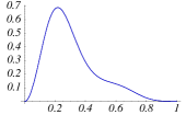
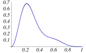
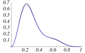
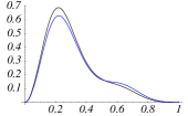
Figure 3: Light intensity for the symmetric superposition of $TE_{0n}$ for $n\in\{1,...,4\}$. The original intensity distribution are plotted in black, the intensity at the Talbot distance $z_{t}=27.7038m$ and its multiples in blue. a) the original intensity; b) 1st Talbot revival; c) 10th Talbot revival; d) 30th Talbot revival; e) 60th Talbot revival; f) 100th Talbot revival.

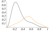
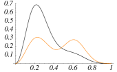
Figure 4: The same superposition as in Fig. 3. The original intensity distribution is plotted in black, in orange are plotted intensities at a) $z=1m,\;$ b) $z=5m,\;$ c) $z=10m.\;$

b) Gaussian “25”

 
Figure 5 presents the revivals of the initial intensity having a Gaussian radial distribution. The Gaussian function was obtained from a superposition of the first 25 $TE_{0.}$ modes. The numerically calculated Talbot distance is $z_{t}=27.7035m$ and the infidelities of revivals (depicted above every plot) are quite low. It is clear that revivals of intensities of a given shape can be observed. Obviously, this result is true only on the assumption that other modes (e.g. modes depending on $\varphi$) do not contribute to the initial image.

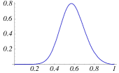
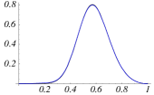
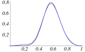
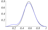
Figure 5: Light intensity for the superposition of $TE_{0n}$, $n\in\{1,...,25\}$, providing a Gaussian distribution. The original intensity distribution are plotted in black, the intensity at the Talbot distance $z_{t}=27.7035$ and its multiples in blue. a) original intensity; b) 1st Talbot revival; c) 10th Talbot revival; d) 30th Talbot revival; e) 60th Talbot revival; f) 100th Talbot revival.

However, the fidelities of revivals depend significantly on the effective number of terms of the Bessel-Fourier (BF) series contributing to the initial image. Although in the example presented above we have taken first 25 terms of the BF series, only first 9 coefficients were larger then $1/1000$ and only first 4 were larger then $1/100$. The coefficients from 11th to 25 were of the order of $5/10000$. If we would like to propagate, say, a more slim Gaussian these proportions would be different. Is is worth noting that in the case of dielectric waveguides this effective number of contributing modes effect not only the fidelities of revivals, but also the optimal Talbot distance, which we will clearly see in the comparison with the next example.

c) symmetric superposition of $TE_{01}+TE_{02}+\dots+TE_{025}$ modes

 
This example of revivals in a thick fiber illustrates how the effective number of contributing modes might modify a Talbot distance. As the initial intensity we take the one corresponding to the symmetric superposition of $TE_{01}+TE_{02}+\dots+TE_{025}$ modes. Figure 6 presents the initial intensity, its 1st Talbot revival and then 10th, 30th, 60th, and 100th Talbot revival. The numerically calculated “optimal” Talbot distance is equal in this case $z_{t}=27.7013m$, which is slightly smaller then in the case presented in examples a), b).

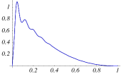
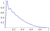
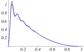
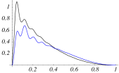
Figure 6: Light intensity for the symmetric superposition of $TE_{0n}$ modes for $n\in\{1,...,25\}$. The original intensity distribution are plotted in black, the intensity at the Talbot distance $z_{t}=27.7013m$ and its multiples in blue. a) the original intensity; b) 1st Talbot revival; c) 10th Talbot revival; d) 30th Talbot revival; e) 60th Talbot revival; f) 100th Talbot revival.

We have already stressed the fact that different initial images have different Talbot distances can be explained by the effective number of modes that are superposed. It is, again, a consequence of importance of the quality of approximations used. In our simplified analysis we have assumed that $\gamma_{n}\simeq\gamma_{0}+n\pi$. On the one hand this is true only for $n$ small enough for $\frac{K_{1}({\kappa})}{\kappa K_{0}({\kappa})}$ plot to be parallel to the $a\gamma$ axis, on the other distance between neighboring zeros of Bessel functions is $\sim\pi$ only for higher modes. Thus, it is obvious that if only first few modes contribute to the initial image (or their contribution dominates) the real Talbot distance would be slightly different then if there were more contributing modes. Differences in optimal Talbot distance $z_{t}$ for superpositions presented in examples a), b), c) can be evaluated explicitly by calculating the infidelities of revivals. They start to be important at 20th, or 50th revival when the initial $2mm$ difference in optimal Talbot distances results in $5$ or $10cm$ divergence from the distance of optimal revival. As long as we are interested only at the first Talbot revival we can take an average $\bar{z}_{t}$ and the infidelities of revivals of different initial images at $\bar{z}_{t}$ should not be larger then 1/100 which is sufficient for most applications. Obviously, when we are interested in revivals at larger distances all the initial images can be divided in classes having the same “effective number of contributing modes” and the revivals at multiples of the corresponding “optimal Talbot distances” would be obtained for all the images within the class.

We have shown numerical simulations indicating that the Talbot revivals of initial images constructed from $TE_{0n}$ modes can be obtained in optical fibers. Although examples a) - c) present superposition of $TE$ modes, one can note that for $TM_{0n}$ modes revivals should be even more faithful, as $\frac{\varepsilon_{1}}{\varepsilon_{2}}<1$ and thus $\gamma_{n}$ are even closer to zeros of $J_{1}(\rho)$ function then it is for TE modes, which brings us to the case of mirror waveguides.

4 Talbot effect in mirror waveguides

Although we present it in the last Section, a model of ideal mirror waveguides is very useful for preliminary calculations. It is analytically soluble for systems of standard geometries because boundary conditions are quite simple: normal component of $\mathbf{B}$ and tangential component of $\mathbf{E}$ have to vanish at the boundary mirror surface.

4.1 Planar mirror waveguides

 
In the elementary case of planar mirror waveguide the propagation constant for $n$th mode is given by $k_{n}^{2}=k_{0}^{2}-\frac{n^{2}\pi^{2}}{d^{2}}$, where $d$ denotes a separation distance between mirrors plates [20, 18]. It is clear that, in general, the field changes its transverse distribution as it travels through the waveguide because different modes travel with different propagation constants and different group velocities. The following expansion of the propagation constant $k_{n}$,

$$k_{n}=\sqrt{k_{0}^{2}-\frac{n^{2}\pi^{2}}{d^{2}}}=k_{0}\sqrt{1-\frac{n^{2}\pi^{2}}{d^{2}k_{0}^{2}}}\simeq k_{0}\left(1-\frac{1}{2}\frac{n^{2}\pi^{2}}{d^{2}k_{0}^{2}}\right),$$ (13)

shows, however, that within this approximation for $z=\frac{4k_{0}d^{2}}{\pi}$ the initial field is obtained. Obviously, requirements for above linear approximation are not met for an arbitrary $k_{n}$. Higher modes have to be prevented from contributing to the image, because only then approximation of the square with accuracy to the linear term is sufficient. The reason why revivals appear is that $\gamma_{i}$ factors are all of the form constant (characterizing the system) times integer. The question arises whether in cylindrical mirror waveguides similar analytical formula for the Talbot distance can be obtained.

Let us note here that necessity of taking care of paraxial approximation is the main difference between optical and quantum mechanical Talbot revivals. In the case of infinite potential well in quantum mechanics, eigenvalues of the system are given by $\frac{n^{2}\pi^{2}}{d^{2}}$ and no excluding of modes (wave functions) that follows from linearization of square root is needed.

4.2 Cylindrical mirror waveguides

 
Solutions of the wave equation in cylindrical mirror waveguides corresponding to angular dependance $e^{\pm i\nu\varphi}$, where $\nu$ denotes a number of Bessel function of a radial solution. Propagating constants are of the form of $\sqrt{{k_{0}^{2}}-\frac{j_{\nu n}^{2}}{a^{2}}}$ for TM modes and $\sqrt{{k_{0}^{2}}-\frac{{j^{\prime}_{\nu n}}^{2}}{a^{2}}}$ for TE modes, where $j_{\nu n}$ denotes the $n$th root of Bessel function $J_{\nu}(x)$ and $j^{\prime}_{\nu n}$ the $n$th root of its derivative and $a$ is a waveguide radius.

In this case not only a linear approximation of square root is needed but also approximation for zeros of Bessel function $j_{\nu n}$ or $j^{\prime}_{\nu n}$. Standard asymptotical expansions for $j_{\nu n}$, $j^{\prime}_{\nu n}$ are given by $j_{\nu n}\simeq n\pi+\left(\nu-\frac{1}{2}\right)\frac{\pi}{2}$ and $j_{\nu n}^{\prime}\simeq n\pi+\left(\nu-\frac{3}{2}\right)\frac{\pi}{2}$. They are believed to be good enough for $n>\nu$ (or in more rigorous manner for $n>2\nu$). Using these formulas we can repeat procedure from Eq. (13) and obtain:

$$\sqrt{k_{0}^{2}-\frac{j_{\nu n}^{2}}{a^{2}}}=k_{0}\sqrt{1-\frac{j_{\nu n}^{2}}{k_{0}^{2}a^{2}}}\approx k_{0}\left(1-\frac{1}{2}\frac{j_{\nu n}^{2}}{k_{0}^{2}a^{2}}\right)\approx k_{0}-\frac{\pi^{2}(4n+2\nu-1)^{2}}{32a^{2}k_{0}}.$$ (14)

Thus,

$$e^{iz\sqrt{{k_{0}^{2}}-\frac{j_{\nu n}^{2}}{a^{2}}}}\approx e^{ik_{0}z}e^{-i2\pi\left(\frac{\lambda}{128a^{2}}\right)(4n+2\nu-1)^{2}z}$$

and

$$(4n+2\nu-1)^{2}=8\biggl{(}2n^{2}+2n\nu-n+\frac{\nu(\nu-1)}{2}\biggr{)}+1.$$

Omitting common phase factor $\exp\big{(}{ik_{0}z+i\frac{2\pi\lambda}{128a^{2}}z}\big{)}$ we find that for a given wavelength $\lambda$ and waveguide radius $a$ at distance $z_{T}={16a^{2}}/{\lambda}$ and its integer multiples Talbot revivals are to be obtained. Similarly, for $TM$ modes approximation for $j^{\prime}_{\nu n}$ leads to the same Talbot distance $z_{T}={16a^{2}}/{\lambda}$.

4.2.1 Examples of revivals in cylindrical mirror waveguides

 
To present the example of the revivals of initial intensity, $I_{org}(0)$, at the Talbot distance and its multiples we have chosen intensity function of the form:

$$I_{org}(0)=\left\{\begin{array}[]{lcl}\sin 2\pi\rho&\mathrm{for}&\rho\in[0,\,0.5),\;\;\varphi\in[0,2\pi[\\ \frac{1}{2}\sin 2\pi\rho&\mathrm{for}&\rho\in(0.5,1],\;\;\,\varphi\in[0,2\pi[.\end{array}\right.$$

Figures 7, 8 show cross-sections for arbitrary $\varphi$ of this initial light intensity $I(0)$ and its Talbot revivals obtained for $ak=10^{3}$ and $ak=10^{4}$, respectively.

 

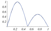
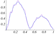
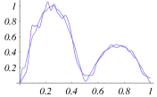
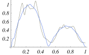
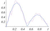
Figure 7: $I(\rho)=\sin(2\pi\rho)$ for $\rho\in[0,\,0.5)$ and $I(\rho)=\frac{1}{2}\sin(2\pi\rho)$ for $\rho\in[0.5,\,1]$. The intensity of light is plotted: $\,a)$ shows initial $I(\rho)$ (an origin and an approximation given by the first 50 terms of BF series, plotted together); $\,b)$ shows the first Talbot revival at $z=z_{T}$ and the initial intensity shown together; $\,c)$, $\,d)$, $\,e)$ show 2nd, 5th, and 10th Talbot revival, respectively.

 

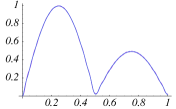
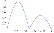
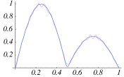
Figure 8: $I(\rho)=\sin(2\pi\rho)$ for $\rho\in[0,\,0.5)$ and $I(\rho)=\frac{1}{2}\sin(2\pi\rho)$ for $\rho\in[0.5,\,1]$. The intensity of light is plotted: $\,a)$ shows initial $I(\rho)$ (an origin and an approximation given by the first 50 terms of BF series, plotted together); $\,b)$ shows the first Talbot revival at $z=z_{T}$ and the initial intensity shown together; $\,c)$, $\,d)$, $\,e)$ show 2nd, 5th, and 10th Talbot revival, respectively.

Analytical function from Eq. (4.2.1) and its approximation by Bessel functions corresponding to $TM_{0i}$ modes are plotted together in Figures 7.a, 8.a. The numerical procedure allowing to approximate a given intensity function we have used here is described in the “Methods” section at the end of the paper. Quality of this approximation, $f_{0}^{a}$, is calculated using measure from Eq. 9. To indicate that the infidelity of approximation is measured, we shall write $f_{0}^{a}$, while the infidelities of revivals defined in a similar way are denoted without this “ ^a ” superscript.

Figures 7.b, 8.b present the first Talbot revival of the initial fields, Figures 7.c, 8.c; 7.d, 8.d; 7.e, 8.e show 2nd, 5th, and 10th Talbot revivals, respectively. Above every plot the corresponding infidelities are depicted. It is very interesting to compare plots and infidelities obtained for the same field distribution, but for different values of $ak$, as it is clearly seen that infidelities are much lower for smaller $\lambda$ to $a$ ratio. This effect is connected with the quality of linear approximation of the square root from Eq. (14). The smaller percentage of all modes is used to construct the initial picture the lower infidelities of higher revivals are to be expected.

4.2.2 Some comments on approximations used

Revivals presented in previous paragraph are quite faithful which means that approximations used to predict the existence of revivals were justified. However, please note, that the examples studied in the previous subsection had the following property: superposed modes were of the same angular dependence (they have corresponded to the Bessel functions of fixed number $\nu$). Studying more complicated combinations one finds out that superpositions of modes with different azimuthal mode numbers do not revive at the Talbot distance [21].

Numerical simulations of field propagation show that the situation is really interesting. As we have already mentioned, superposition of TM or TE modes having the same angular dependance revive quite faithfully at Talbot distance and only for the superpositions of “mismatched” modes revivals are not obtained. Explanation of this surprising fact is the following: the higher terms of the asymptotic formulae for the roots of Bessel functions, and its derivatives [22]:

$$j_{\nu n}=\underbrace{n\pi+\bigg{(}\nu-\frac{1}{2}\bigg{)}\frac{\pi}{2}}_{A}-\underbrace{\frac{4\nu^{2}-1}{8\left(n\pi+\big{(}\nu-\frac{1}{2}\big{)}\frac{\pi}{2}\right)}}_{B}-\underbrace{\frac{(4\nu^{2}-1)(28\nu^{2}-31)}{384\left(n\pi+\big{(}\nu-\frac{1}{2}\big{)}\frac{\pi}{2}\right)^{3}}}_{C}-...$$ (15)

and

$$j^{\prime}_{\nu n}=\underbrace{n\pi+\bigg{(}\nu-\frac{3}{2}\bigg{)}\frac{\pi}{2}}_{A^{\prime}}-\underbrace{\frac{4\nu^{2}+3}{8\left(n\pi+\big{(}\nu-\frac{3}{2}\big{)}\frac{\pi}{2}\right)}}_{B^{\prime}}-\underbrace{\frac{112\nu^{4}+328\nu^{2}-9}{384\left(n\pi+\big{(}\nu-\frac{3}{2}\big{)}\frac{\pi}{2}\right)^{3}}}_{C^{\prime}}-...$$ (16)

are more important then we have assumed so far. In many papers and textbooks only first terms ($A,\,A^{\prime}$) of above approximations are used and we have also limited ourselves to them in preliminary calculations but to obtain a faithful approximation at least two first terms should be taken into account. From formulas (15), (16) it is, however, clear that when higher terms are taken into account, finding the Talbot distance for arbitrary $\nu$ and $n$ fails, because different powers of $\pi$ would be included.

So how we can observe any revivals at all? Let us take a closer look at approximation (16), i.e. one considering TE modes – keeping in mind that similar analysis can be made for TM modes as well. Taking two first terms of approximation (16) the following expression for ${j^{\prime}}_{\nu n}^{2}$ is obtained:

$${j^{\prime}}_{\nu n}^{2}=\underbrace{\left(n\pi+\bigg{(}\nu-\frac{3}{2}\bigg{)}\frac{\pi}{2}\right)^{2}}_{{A^{\prime}}^{2}}-\underbrace{\frac{4\nu^{2}+3}{4}}_{2A^{\prime}B^{\prime}}+\underbrace{\frac{(4\nu^{2}+3)^{2}}{64\left(n\pi+\big{(}\nu-\frac{3}{2}\big{)}\frac{\pi}{2}\right)^{2}}}_{{B^{\prime}}^{2}}$$ (17)

Ratios ${B^{\prime}}^{2}/{A^{\prime}}^{2}$ and $2A^{\prime}B^{\prime}/{A^{\prime}}^{2}$ for a wide range of parameters $\nu$ and $n$ are shown in Figure 9. It is seen that although the ratio ${B^{\prime}}^{2}/{A^{\prime}}^{2}$ for $n>\nu$ is close to zero and can be neglected, the percentage value of $2B^{\prime}/A^{\prime}$ can be quite significant.

   

   

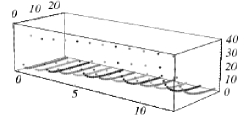
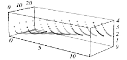
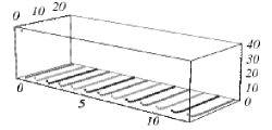
Figure 9: Errors of “asymptotic” approximation of $(j^{\prime}_{\nu n})^{2}$: Notation is taken from from Eqs. 16, 17: Plots a) and b) show in two different scales percentage ratio of $2B^{\prime}/A^{\prime}$ for $\nu\in\{0,...,12\}$, $n\in\{1,...,25\}$. Unicolor dotted lines correspond to one value of azimuthal mode number $\nu$. Plots c) and d) present percentage ratio of ${B^{\prime}}^{2}/{A^{\prime}}^{2}$. It is seen that for $n>\nu$ this term can be neglected.

Obviously, this is the effect we were looking for as term $2A^{\prime}B^{\prime}=\nu^{2}+\frac{3}{4}$ depends only on the azimuthal mode number $\nu$ and not on the radial one $n$. That is the reason why modes having the same angular dependence revive at the Talbot distance $z_{T}=\frac{16}{\lambda}$, while for a superposition of modes with different angular dependence we do not obtain such revivals. In the first case factor $\exp\left(-i(4\nu^{2}+3)z_{T}/4\right)$ is merely a phase common for all the terms of the superposition. When the initial $H_{z}$ is the superposition of a form $H_{z}(0)=J_{\nu}(j^{\prime}_{\nu n}\rho)e^{i\nu\varphi}+J_{\mu}(j^{\prime}_{\mu m}\rho)e^{i\mu\varphi}\;$ then at $z=z_{T}$ phase factors corresponding to $J_{\nu}$ and $J_{\mu}$ differ for $\nu\neq\mu$ and, consequently, they do not cancel. This relative phase destroys the Talbot revivals promised by less accurate approximation.

Similar analysis shows that superpositions of $TM$ and $TE$ modes will not revive at the same distance because of the relative phase. Only for $TM_{1i}$ and $TE_{0j}$ modes this relative phase disappears and Talbot effect can be observed. However, due to possibility of using polarizers, restrictions imposed by necessity of choosing polarization of modes used is experimentally less demanding then that concerning $\varphi$-dependance.

5 Summary

We have discussed in details approximations that appear in the study of the Talbot effect in the cylindrical mirror waveguides as well as different approximations used in the case of dielectric waveguides. We have shown that in many cases almost perfect revivals can be obtained and that even dephased propagation can be used in practice. We have stressed that a phase space description (sometimes regarded as an unnecessary complicated representation) extracts an essence of the interference phenomena and that the conditions needed to be fulfilled to obtain Talbot revivals in a very natural way follow from a phase space description of interference.

6 Methods

The following numerical procedure was used for decomposing given initial light intensity $I_{org}$ into $TM_{0i}$ modes: For an arbitrary spherically symmetric $TM$ field with an initial $E_{z}$ of a form

$$E_{z}(0)=\sum_{i=1}^{50}x_{i}J_{0}(j_{0i}\,\rho)$$ (18)

we have evaluated the light intensity $I(0)$ and this $I(0)$ was expanded again in a Bessel-Fourier series corresponding to $J_{0}$. Numerical evaluation of some integrals was required at this point. In such a way general “basis” $(e_{1},e_{2},...,e_{50})$ was obtained, (every $e_{i}$ being a sum of all possible pairs $x_{i}\cdot x_{j}$ with numerically calculated coefficients). Then, an arbitrary $\varphi$-independent intensity $I_{org}$ that we would like to propagate through the waveguide was decomposed in BF series

$$I_{org}(0)\approx\sum_{i=1}^{50}c_{i}J_{0}(j_{0i}\rho),$$ (19)

and a set of quadratic equations $c_{1}=e_{1}$, $c_{2}=e_{2},\,\cdots\,,$ $c_{50}=e_{50}$ was solved numerically to find $(x_{i})_{i=1}^{50}$. Figures 7.a, 8.a can be treated as a test of faithfulness of the solutions founded in the procedure described above – the infidelities of approximation $f_{0}^{a}$ are of the order of $10^{-2}$.

7 Acknowledgements

We would like to acknowledge useful discussions with Professor W. P. Schleich. This research was partially supported by Polish MEN Grant No. 1 P03B 137 30 and European Union’s Transfer of Knowledge project CAMEL (Grant No. MTKD-CT-2004-014427).

References

- [1] W. H. Fox Talbot, Philos. Mag. 9 no. IV (1836) 401-405
- [2] Lord Rayleigh, Philos. Mag. 11 (1881) 196-205
- [3] M. Wolfke, Ann. Phys. (Germany) 40 (1913) 194-200 and references therein
- [4] K. Patorski, The Self-Imaging Phenomenon and Its Applications, in: E. Wolf (ed.), Progress in Optics, vol. 27, 3-108, North Holland, Amsterdam 1989
- [5] R. W. Robinett, Phys. Rep. 392 (2004) 1-119
- [6] M. V. Berry, S. Klein, J. Mod. Opt. 43 (1996) 2139 - 2164
- [7] K. Banaszek, K. Wódkiewicz, W. Schleich, Opt. Express 2 (1998) 169-172
- [8] M. V. Berry, J. Phys. A 29 (1996) 6617-6629
- [9] I. Marzoli et al., Acta Physica Slov., vol. 48, No. 3, (1998) 323-333
- [10] M. Berry, I. Marzoli, W. Schleich, Phys. World, vol. 14, no. 6, (2001), 39-44
- [11] R. Ulrich, Opt. Commun. 13, no. 3, (1975), 259-264
- [12] B. Rohwedder, Phys. Rev. A 63 (2001) 053604
- [13] J. D. Jackson, Classical Electrodynamics, John Wiley & Sons, 1975
- [14] E. Wigner, Phys. Rev. 40 (1932) 749-759
- [15] W. P. Schleich, Quantum Optics in Phase Space, Wiley-vch, 2001
-
[16]
J. G. Kirkwood, Phys. Rev. 44 (1933) 31-37
A. N. Rihaczek, IEEE Trans. Inf. Theory 14 (1968) 369-374 - [17] L. Praxmeyer, K. Wódkiewicz, Opt. Commun. 223 (2003) 349-365
- [18] Peter K. Cheo, Fiber Optics and Optoelectronics, Prentice-Hall International Editions, 1990
- [19] C. D. Cantrell, Dawn M. Hollenbeck, Fiberoptic Mode Functions: A Tutorial, www.utdallas.edu/ cantrell/ee6328/modefunctions.pdf
- [20] B. E. A. Saleh, M. C. Teich, Fundamentals of Photonics, John Wiley & Sons, 1991
- [21] L. Praxmeyer, Classical and quantum interference in phase space, PhD thesis, 2005.
- [22] F. W. J. Olver, Introduction to asymptotics and special functions, Academic Press, 1974