Asymmetries in Mars’ Exosphere

Abstract

Observations and simulations show that Mars’ atmosphere has large seasonal variations. Total atmospheric density can have an order of magnitude latitudinal variation at exobase heights. By numerical simulations we show that these latitude variations in exobase parameters induce asymmetries in the hydrogen exosphere that propagate to large distances from the planet. We show that these asymmetries in the exosphere produce asymmetries in the fluxes of energetic neutral atoms (ENAs) and soft X-rays produced by charge exchange between the solar wind and exospheric hydrogen. This could be an explanation for asymmetries that have been observed in ENA and X-ray fluxes at Mars.

1 Introduction

Traditionally, exospheric densities and velocity distributions are modelled by spherical symmetric analytical Chamberlain functions (Chamberlain and Hunten, 1987). Chamberlain theory assumes that gravity is the only force acting on the neutrals, that the exobase parameters (density and temperature) are uniform over a spherical exobase, and that no collisions occur above the exobase. Planetary exospheres are however not spherical symmetric due to non-uniform exobase parameters and due to effects such as photoionization, radiation pressure, charge exchange, recombination and planetary rotation. To account for these effects numerical simulations are needed. Using Monte Carlo test particle simulations it is possible to account for the above effects (if ion distributions are assumed).

Even though neutrals in the exospheres by definition do not collide often, collisions occur. Especially near the exobase the transition is gradual from collision dominated regions at lower heights (with Maxwellian velocity distributions) to essentially collisionless regions at greater heights. Using test particles one can model collisions with an assumed background atmospheric profile (Hodges Jr., 1994), but to account for collisions properly the test particle approach is not sufficient, and self consistent simulations are needed. One approach to model collisions is the direct simulation Monte Carlo (DSMC) method (Bird, 1976) for rarefied flows, that has been applied to exospheres by Krestyanikova and Shematovich (2005).

In this work we use the test particle approach to model the effects on the Martian exosphere from non-uniform exobase conditions, from photoionization, from radiation pressure, and from solar wind charge exchange. We launch test particles from the exobase and follow their trajectories. The forces on the particles are from gravity and radiation pressure. Along their trajectories the particles can be photoionized, and they can charge exchange with solar wind protons outside the bow shock. Exospheric column densities give us a qualitative estimate of how exospheric asymmetries effect solar wind charge exchange (SWCX) X-ray images. The energetic neutral atoms (ENAs) produced by charge exchange then gives us estimates of the ENA fluxes near Mars.

In this work we do not include the effects of collisions since it greatly increases the computational cost. Collisions and photochemical reactions are two channels, in addition to charge exchange, that produce an hot hydrogen population (Nagy et al, 1990). By only including charge exchange outside the bow shock as a source of hot hydrogen in this work we therefore under estimate the extent of the hydrogen corona. Including all sources of hot hydrogen would result in more extended emissions of ENAs and X-rays, compared to the results presented here. An additional process that we do not consider is electron impact ionization, since it would require knowledge of electron fluxes and velocity distributions. However, this work should be seen as a first qualitative study of how asymmetries in exobase conditions at Mars effect the exosphere, and in turn the ENA and X-ray fluxes near Mars. To do a more accurate quantitative study is much more difficult. One then would need to specify the exact time, season and Mars–Sun distance; and have access to exobase conditions (at that time) from observations, global circulation models, and solar wind conditions, along with full knowledge of the ion fluxes near Mars.

1.1 ENA and X-ray imaging

When the solar wind encounters a non-magnetized planet with an atmosphere, e.g., Mars or Venus, there will be a region of interaction, where solar wind ions collide with neutrals in the planet’s exosphere. Two of the processes taking place are

• The production of ENAs by charge-exchange between a solar wind proton and an exospheric neutral (Holmström et al, 2002), and

• The production of soft X-rays by SWCX between heavy, highly charged, ions in the solar wind and exospheric neutrals (Holmström et al, 2001).

Images of ENAs and SWCX X-rays can provide global, instantaneous, information on ion-fluxes and neutral densities in the interaction region. It is however not easy to extract this information from the measured line of sight integrals that are convolutions of the ion-fluxes and the neutral densities. We need to introduce models that reduce the complexity of the problem. At Mars, the hydrogen exosphere is enlarged due to the planet’s low gravity, and thus provide a large interaction region, extending outward several planet radii. Traditionally, most of the modeling of the outer parts of Mars’ exosphere has been using analytical, spherical symmetric, Chamberlain profiles. Planetary exospheres are however not spherical symmetric to any good approximation, and asymmetries at Mars observed in ENAs by Mars Express and in X-rays by XMM-Newton could be due to asymmetries in the exosphere. The neutral particle imager, part of ASPERA-4 on-board Mars Express, has observed asymmetries in the ENA fluxes in the shadow of the planet (Brinkfeldt et al, 2006). The decline of ENA fluxes when entering the shadow is different from the rise in flux when exiting the shadow. The XMM Newton X-ray telescope observed Mars in November 2003, and SWCX X-rays were positively identified from the hydrogen corona (Dennerl et al, 2006). The morphology of the images are however different from what have been predicted by simulations (Holmström et al, 2001). One of the differences is that the emissions are asymmetric with respect to the ecliptic plane. Here we investigate the asymmetries in exospheric densities at Mars due to various factors, and their impact on ENA and SWCX X-ray images.

We may note that although asymmetric exospheres have not been used often in modeling of solar wind-Mars interactions, they are well known in the engineering community since aerobraking and satellite drag is directly dependent on exospheric densities, and provides total density measurements (Justus et al, 2002).

In Section 2 we describe in more detail the methods and parameters used in our simulations. In Section 3 we then present the results of our numerical experiments, and finally we present conclusions in Section 4.

2 Methods

Here we first describe the algorithms used to simulate Mars’ hydrogen exosphere, and we then describe the detailed setup used in the numerical experiments.

2.1 The simulation algorithm

In what follows, the coordinate system used is Mars solar ecliptic coordinates, centered at the planet with the $x$-axis toward the Sun, the $z$-axis perpendicular to the planet’s velocity, in the northern ecliptic hemisphere, and a $y$-axis that completes the right handed system. Based on this solar ecliptic coordinate system we define (longitude, latitude) coordinates, with the $z$-axis toward 90 degree latitude, the $x$-axis (sub solar point) at (0,0), and the $y$-axis at (90,0).

The simulation domain is bounded by two spherical shells centered at Mars. An inner boundary (the exobase) with a radius of 3580 km corresponding to a height of 200 km above the planet – assuming from now on a planet radius $R_{M}$ of 3380 km – and an outer boundary with a radius of 10 $R_{M}$. At the start of the simulation the domain is empty of particles. Then meta-particles are launched from the inner boundary at a rate of 1000 meta-particles per second. Each meta-particles corresponds to $N_{m}$ hydrogen atoms. The location on the inner boundary of each launched particle is randomly drawn with probability proportional to the local hydrogen exobase density. The velocity of each launched particle is randomly drawn from a probability distribution proportional to

$$\left(\mathbf{n}\cdot\mathbf{v}\right)e^{-a|\mathbf{v}|^{2}},$$

where $\mathbf{n}$ is the local unit surface normal, $\mathbf{v}$ is the velocity of the particle, and $a=m/(2kT)$, $m$ is the mass of a neutral, $k$ is Boltzmann’s constant, and $T$ is the temperature (at the exobase position). Note that the distribution used is not a Maxwellian, but the distribution of the flux through a surface (the exobase) given a Maxwellian distribution at the location (Garcia, 2000).

After an hydrogen atom is launched from the inner boundary, we numerically integrate its trajectory with a time step of 5 seconds. To avoid energy dissipation, the time advance of the particles is done using a fourth order accurate symplectic integrator derived by Candy and Rozmus (1991).

Between time steps, the following events can occur for an exospheric atom

• Collision with an UV photon. Following Hodges Jr. (1994) this occurs as an absorption of the photon ($\Delta v$ opposite the sun direction) followed by isotropic reradiation ($\Delta v$ in a random direction). From Hodges Jr. (1994) we use a velocity change $\Delta v=3.27$ m/s. The collision rate used is $10^{-3}$ s^-1, and the rate is zero if the particle is in the shadow behind the planet.

• Charge exchange with a solar wind proton. If the hydrogen atom is outside Mars’ bow shock it can charge exchange with a solar wind proton, producing an ENA, at a rate of $8.4\cdot 10^{-8}$ s^-1. The ENA is randomly drawn from a Maxwellian velocity distribution with a bulk velocity of 450 km/s in the anti-sunward direction, and a temperature of $1.2\cdot 10^{5}$ K. Thus, the original exospheric hydrogen atom is replaced by the ENA in the simulation. Following Slavin et al (1991), we define the bow shock by the surface $(x,\rho)$ $R_{M}$ such that

  $$x=\frac{-x_{0}+Le+x_{0}e^{2}-\sqrt{\rho^{2}e^{2}-\rho^{2}L^{2}}}{e^{2}-1},$$

  where $L=2.04$ $R_{M}$, $e=1.02$, and $x_{0}=0.55$ $R_{m}$. Here $\rho=\sqrt{y^{2}+z^{2}}$ is the distance to the $x$-axis (the Mars–Sun line). We can note that the charge exchange rate gives an average life time for an hydrogen atom of more than 100 days in the solar wind. The implication for our simulations is that few ENA meta-particles are produced. To handle this we increase the charge exchange rate by a factor of $f=1000$ and when a charge exchange event occurs, the exospheric meta-particle with weight $N_{m}$ is replaced by a meta-particle with weight $(1-1/f)N_{m}$ and an ENA with weight $N_{m}/f$.

• Photoionization by a solar photon occurs at a rate of $10^{-7}$ s when an exospheric hydrogen atom is outside the optical shadow behind the planet, and then the meta-particle is removed from the simulation.

All rates above are from Hodges Jr. (1994) for Earth, and average solar conditions, scaled by 0.43 to account for the smaller fluxes at Mars. For a given event rate, $\tau$, after each time step, for each meta-particle, we draw a random time from an exponential distribution with mean $\tau$, and the event occur if this time is smaller than the time step. Note that we only consider ENAs produced outside the bow shock, so the fluxes presented here is a lower bound. Additional ENAs are produced inside the bow shock, but including those would require a complete ion flow model. Anyhow, simulations (Holmström et al, 2002) suggest that the ENA flux from the solar wind population is dominant in intensity. Also, we do not consider collisions between neutrals, as discussed in the introduction. We can note that omitting collisions means that the population of particles on satellite orbits will be small. The only generation mechanism for satellite particles will be radiation pressure.

2.2 The simulation setup

As stated in the introduction, the aim of this study is to make a qualitative study of the effects of non-uniform exobase conditions on the hydrogen exosphere, and the implications for ENA and SWCX X-ray fluxes. Thus, we choose to study a simplified model problem where we have artificially chosen a spatial distribution of exobase density and temperature, shown in Figure 1.

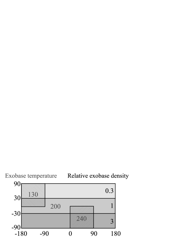
Figure 1: The non-uniform exobase density and temperature for Mars’ hydrogen exosphere used in this study. The coordinate system is Mars solar ecliptic longitude and latitude, with (0,0) corresponding to the sub solar point. The exobase temperature is shown in gray, with a value of 200 K, except for a region of increased temperature on the dayside, and a region of decreased temperature on the nightside. The exobase density is constant in three longitude bands, and shown in black is the density relative to a reference density of $4.2\cdot 10^{5}$ cm^-3.

We have constant density in three longitude bands, and three different temperature regions. This is an approximation of the conditions at southern summer solstice, and was chosen as follows. We use the density and temperature for solar minimum conditions from (Krasnopolsky, 2002, Fig. 1) at a height of 200 km; 200 K and $4.2\cdot 10^{5}$ cm^-3 as a reference value. This is a day side average for a solar zenith angle of 60 degrees. The corresponding density at 130 km (mostly CO₂) is 2.9 kg/km³. Using the spatial variations from (Bougher et al, 2000, Fig. 5 and 10) we scale the reference values, and construct the exobase conditions shown in Figure 1. We will later denote this the non-uniform case, and the case when we use the reference values for all of the exobase will be the uniform case. The spatial variations in (Bougher et al, 2000) are from a global circulation model of Mars’ exosphere and is based on the observations available at that time. Later the model has been partially verified by observations (Lillis et al, 2005). Note that these exobase parameters specify the upward velocity distribution of neutrals at the inner boundary (the exobase). The downward flux is then obtained from the simulation. Therefore, these parameters will differ from the values obtained from the converged simulation, e.g., we can see in Figure 2 that the number density at the inner boundary has the proportions 1, 3, and 7 in the different latitude bands.

3 Numerical experiments

First we investigate the effects of non-uniform exobase conditions on the hydrogen exosphere. Then we study the implications for ENA and SWCX X-ray fluxes.

3.1 The exosphere

Here we use the non-uniform exobase conditions shown in Figure 1. First of all we want to examine how far out from the planet the exosphere is non-uniform. Since the simulation particles are launched on ballistic trajectories, at any point there will be a mix of particles from different regions of the exobase. This will introduce a smoothing of the exobase boundary conditions, and it is not obvious how large this smoothing will be, i.e. how far from the planet the non-uniformity will persist. To investigate this we divide the exosphere into three regions corresponding to the three latitude bands in Figure 1, and plot profiles of the average hydrogen density for each of the regions. These profiles at a time of 10 hours after the start of the simulation are shown in Figure 2.

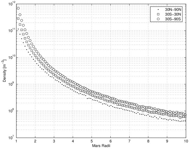
Figure 2: Average hydrogen number density [m^-3] as a function of planetocentric distance in $R_{M}$ for non-uniform exobase conditions. The exosphere has been divided into three regions corresponding to the three latitude bands in Figure 1, and each of the profiles shown is an average over the corresponding region. Latitude 30 to 90 degrees (dots), -30 to 30 (squares), and -90 to -30 (circles).

We see that the density variation at the exobase by a factor of 10 is reduced to approximately a factor of 3 at a planetocentric distance of 2 $R_{M}$, and a factor of 2 at 10 $R_{M}$. Thus, the exospheric densities get more uniform with distance to the planet, but large differences in density persist all through the simulation domain.

3.2 SWCX X-rays

To estimate the effects of the non-uniform exosphere on SWCX X-ray images, we note that the X-ray flux is a line-of-sight convolution of ion flux and hydrogen density. So in the unperturbed solar wind, outside the bow shock, the X-ray flux should be proportional to the hydrogen column density. In Figure 3 we show the hydrogen column density for the cases of uniform and non-uniform exobase conditions. These are then estimates of what SWCX X-ray images would look like, from Earth at Mars’ opposition, at least away from the planet (near the planet X-ray fluorescence dominate anyway). Note that the column density can vary by almost an order of magnitude, for constant planetocentric distances, even far away from the planet, in the non-uniform case. This would directly effect SWCX X-ray images and lead to asymmetries of the same magnitude.

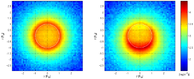
Figure 3: Logarithm of the hydrogen column density [m^-2] along the $x$-axis for uniform (left) and non-uniform (right) exobase conditions. The white circles shows the size of the exobase. The time is 10 hours, the axes’ units are $R_{M}$ and the total number of meta-particles are 848320 and 893240. The maximum column density is 0.781 and 1.86 $\cdot 10^{14}$m^-2.

3.3 ENA fluxes

Here we investigate the fluxes of hydrogen ENAs that are created outside the bow shock by charge exchange between exospheric hydrogen and solar wind protons, with respect to any asymmetries induced by the asymmetric exosphere. One motivation for this investigation is that the neutral particle imager, part of ASPERA-4 on-board Mars Express, has seen asymmetries in the ENA fluxes in the tail behind the planet (Brinkfeldt et al, 2006). In Figure 4 we compare the ENA fluxes through a plane at $x=-1.0$ for uniform and non-uniform exobase conditions.

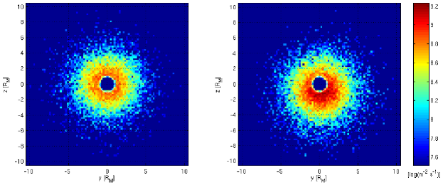
Figure 4: Logarithm of the ENA fluxes [m^-2s^-1] through the $yz$-plane at $x=-1.0$ $R_{M}$ for uniform exobase conditions (left), and for non-uniform conditions (right). The maximum flux is $0.912$ and $1.79$ $\cdot 10^{9}$m^-2s^-1. The fluxes are computed by averages over all ENAs with $-1.05<x<-0.95$, from time 0 to 10 hours, the axes’ units are $R_{M}$, and the total number of ENA meta-particles is 18796 and 22924. The white circle shows the size of the exobase.

We can note the spherical symmetry for the case of uniform exobase conditions, apart from the statistical fluctuations associated with test particle Monte Carlo simulations. On the other hand, in the case of non-uniform exobase parameters the asymmetry of the ENA flux is clearly visible as enhanced, and extended, flux in the south corresponding to the higher densities in the southern hemisphere. There is also a suggestion of enhanced densities in the $+y$ hemisphere corresponding to the enhanced exobase temperature in that hemisphere. For a constant planetocentric distance in this plane we see that the ENA flux can vary by more than a factor of 2.

How does the ENA fluxes vary at different positions relative to the planet? In Figure 5 we plot the fluxes through the $yz$-planes at $x=$ 1.0, 0.0, -1.0, and -3.0.

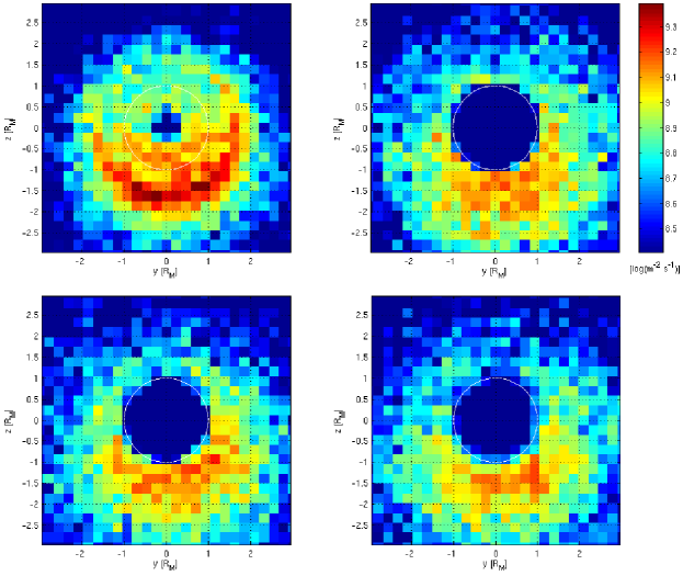
Figure 5: Logarithm of the ENA fluxes [m^-2s^-1] through the $yz$-planes at $x=1$ $R_{M}$ (upper left), $x=0$ (upper right), $x=-1$ (lower left), and $x=-3$ (lower right) for non-uniform exobase conditions. All are averages over an $x$-width of 0.1 $R_{M}$. The maximum fluxes are 2.50, 1.63, 1.79, and 1.60 $\cdot 10^{9}$m^-2s^-1. The white circle shows the size of the exobase.

The north-south asymmetry is visible in all plots, with the highest, most concentrated fluxes at $x=1$. The area of large flux then spreads out slightly and has a bit lower intensity toward the tail. Note however that the flux at $x=-3$ is as large as the flux at $x=0$. For all plots the maximum flux seems to be obtained at an approximate distance from the $x$-axis of 5000 km (about 1600 km outside the optical shadow). This is perhaps a bit surprising — that the maximum flux is not closer to the umbra, but is a consequence of the shape of the bow shock in combination with the exospheric profiles, as seen in the flux through $x=1$ that is a crescent well outside the planet outline.

In all numerical experiments above, radiation pressure and photoionization was not included. It was found that including those events, as described in the previous section, did not change the results presented in any significant way.

4 Conclusions

Traditionally, modeling of the solar wind interaction with Mars’ exosphere, and the production of SWCX X-rays and ENAs, has assumed a spherical symmetric exosphere. From observations and simulations we know however that the exosphere is not symmetric. From the results of our simple test particle model of Mars’ exosphere we find that asymmetries in exobase density and temperature propagate to large heights (many Martian radii). Column densities can deviate by almost an order of magnitude from symmetry, implying similar asymmetries in SWCX X-ray images. We also find that the fluxes of ENAs that are produced in the solar wind can deviate by more than a factor of two from symmetry. These asymmetries could explain the asymmetries seen in X-ray images and in ENA observations, but further studies are needed to find out if that is the case. We also find that radiation pressure and photoionization are unimportant processes in comparison to asymmetries in exobase parameters. Finally, we can note that asymmetries in the exosphere could also possibly explain the low exospheric densities seen by the neutral particle detector on-board Mars Express, as reported in this issue by Galli et al (2006), since that measurement was over the northern hemisphere during early northern spring (April 25, 2004), when exospheric densities should have been low due to the seasonal variations.