Simulation of Three Dimensional Electrostatic Field Configuration in Wire Chambers : A Novel Approach

Abstract

Three dimensional field configuration has been simulated for a simple wire chamber consisting of one anode wire stretched along the axis of a grounded square cathode tube by solving numerically the boundary integral equation of the first kind. A closed form expression of potential due to charge distributed over flat rectangular surface has been invoked in the solver using Green’s function formalism leading to a nearly exact computation of electrostatic field. The solver has been employed to study the effect of several geometrical attributes such as the aspect ratio ($\lambda=\frac{l}{d}$, defined as the ratio of the length $l$ of the tube to its width $d$) and the wire modeling on the field configuration. Detailed calculation has revealed that the field values deviate from the analytic estimates significantly when the $\lambda$ is reduced to $2$ or below. The solver has demonstrated the effect of wire modeling on the accuracy of the estimated near-field values in the amplification region. The thin wire results can be reproduced by the polygon model incorporating a modest number of surfaces ($\geq 32$) in the calculation with an accuracy of more than $99\%$. The smoothness in the three dimensional field calculation in comparison to fluctuations produced by other methods has been observed.

,

1 Introduction

Wire chambers are often employed as tracking devices where it is necessary to detect and localize radiation. Starting from its application in nuclear and subnuclear physics, it has been employed in widely different fields such as biology, medicine, space, industrial radiology, over last three decades or more. The normal operation of a wire chamber is based on the collection of the charges created by direct ionization of the gas medium by the passage of radiation. The charges are collected on the electrodes by application of an electric field across the chamber. From the electric pulses, thus generated, the relevant information regarding the radiation is extracted. The flexibility in the design of wire chambers allows for highly innovative and often considerably complex ones necessitating meticulous investigations on their structure and performance. The study of the electrostatic field plays a key role in optimizing the design of these state of the art detectors to get a desired configuration for the field in a given volume as per the tracking requirement. The analytic solution of the field configuration for a specific geometry is always the best choice to do the same. However, the analytic solution can be derived for severely restricted geometries which is often not applicable to realistic and complicated wire chambers [1, 2]. The diversity in the chamber design necessitates application of other techniques for numerical estimation like Finite Element Method (FEM) and Finite Difference Method (FDM) [3, 4]. FEM is more widely used for the reason that it can seamlessly handle any arbitrary geometry including even dielectrics. However, FEM has several drawbacks as well. It computes the potential at the nodes and the potential at non-nodal points can be obtained by interpolation only. The inaccuracy generated by the interpolation technique can be made arbitrarily small by proper meshing techniques at the cost of computation time and efficiency. The more crucial aspect which harms the accuracy of the estimation is the representation of the electric field by a low order, often linear polynomial which is inadequate especially in the vicinity of the wires where the field changes rapidly. The combination of inadequate representation of the electric field and poor meshing lead to inaccurate estimation of the field in the amplification region with the FEM technique. The other approach which can yield nominally exact result is Boundary Integral Equation (BIE) method. This method is less popular due to its complicated mathematics and inaccuracies near the boundaries. However, for the present problem of computation of electrostatic field in wire chambers, BIE method is reasonably more suitable. It can provide accurate estimate of the electrostatic field at any arbitrary point by employing Green’s function formulation which is necessary to study the avalanche happening anywhere in the chamber due to the passage of radiation. A brief comparison of BEM, the numerical implementation of BIE method, with FEM and FDM in the context of calculating three dimensional field configuration in wire chambers has been presented in [5].

The major drawback of BEM is related to the approximations involved in its numerical implementation. The approximations give rise to the infamous numerical boundary layer where the method suffers from gross inaccuracies [6]. This may lead to inaccurate estimation of electrostatic field configuration which is not desirable in the close vicinity of the wires or the cathode. Recently, we have developed a novel approach in the formulation of BEM using analytic expressions for potential and electrostatic field which leads to their nominally exact evaluation. The analytic expressions being valid throughout the physical volume, the formulation is capable of yielding accurate values even in the near-field region. The application of this Nearly Exact Boundary Element Method (NEBEM) solver [7] for the very accurate estimation of electrostatic field in a wire chamber of elementary but useful geometry has been presented in this paper.

2 Present Approach

For electrostatic problems, the BIE can be expressed as

$$\phi(\vec{r})=\int_{S}G(\vec{r},\vec{r}^{\prime})\rho(\vec{r}^{\prime})dS^{\prime}$$ (1)

where $\phi(\vec{r})$ represents potential at $\vec{r}$ integrating the integrand over boundary surface $S$, $\rho(\vec{r}^{\prime})$ the charge density at $\vec{r}^{\prime}$ and $G(\vec{r},\vec{r}^{\prime})=1/4\pi\epsilon|\vec{r}-\vec{r}^{\prime}|$ with $\epsilon$ being the permittivity of the medium. The BIE is numerically solved by discretizing the charge carrying surface $S$ in a number of segments on which uniform charge densities $\rho$ are assumed to be distributed. The discretization leads to a matrix representation of the BIE as follows

$$\mathbf{A}\cdot\mathbf{\rho}=\mathbf{\phi}$$ (2)

where $A_{ij}$ of $\mathbf{A}$ represents the potential at the mid-point of segment $i$ due to a unit charge density distribution at the segment $j$. For known potential $\mathbf{\phi}$, the unknown charge distribution $\mathbf{\rho}$ is estimated by solving Eqn.(2) with the elements of influence matrix $\mathbf{A}$ modeled by a sum of known basis functions with constant unknown coefficients.

In the present approach, namely NEBEM, the influences are calculated using analytic solution of potential and electrostatic field due to a uniform charge distribution over a flat rectangular surface. The expression for the potential $\phi$ at a point $P(X,Y,Z)$ in free space due to uniform unit charge density distributed on a rectangular surface having corners at $(x_{1},0,z_{1})$ and $(x_{2},0,z_{2})$ as shown in Fig.1 can be represented as a multiple of

$$\phi(X,Y,Z)=\int_{z_{1}}^{z_{2}}\int_{x_{1}}^{x_{2}}\frac{dx\,dz}{\sqrt{(X-x)^{2}+Y^{2}+(Z-z)^{2}}}$$ (3)

where the multiple depends upon the strength of the source and other physical considerations. The closed form expression for $\phi(X,Y,Z)$ can be deduced from the Eqn.(3).

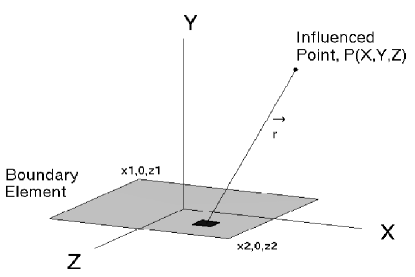
Figure 1: A rectangular surface with uniform distributed source

This can be expressed as follows.

$$\phi(X,Y,Z)=$$ (4)

$$(X-x_{1})\,\ln\left(\frac{D_{12}\,-\,(Z-z_{2})}{D_{11}\,-\,(Z-z_{1})}\right)+(X-x_{2})\,\ln\left(\frac{D_{21}\,-\,(Z-z_{1})}{D_{22}\,-\,(Z-z_{2})}\right)$$

$$+(Z-z_{1})\,\ln\left(\frac{D_{21}\,-\,(X-x_{2})}{D_{11}\,-\,(X-x_{1})}\right)+(Z-z_{2})\,\ln\left(\frac{D_{12}\,-\,(X-x_{1})}{D_{22}\,-\,(X-x_{2})}\right)$$

$$+\frac{i\,|Y|}{2}$$

$$\left(\right.S_{1}\,\left(\right.tanh^{-1}\left(\frac{R_{1}+i\,I_{1}}{D_{11}\,\left|Z-z_{1}\right|}\right)-\,tanh^{-1}\left(\frac{R_{1}-i\,I_{1}}{D_{11}\,\left|Z-z_{1}\right|}\right)$$

$$+\,tanh^{-1}\left(\frac{R_{1}-i\,I_{2}}{D_{21}\,\left|Z-z_{1}\right|}\right)-\,tanh^{-1}\left(\frac{R_{1}+i\,I_{2}}{D_{21}\,\left|Z-z_{1}\right|}\right)\left.\right)$$

$$+\,S_{2}\,\left(\right.tanh^{-1}\left(\frac{R_{2}+i\,I_{2}}{D_{22}\,\left|Z-z_{2}\right|}\right)\,-\,tanh^{-1}\left(\frac{R_{2}-i\,I_{2}}{D_{22}\,\left|Z-z_{2}\right|}\right)$$

$$+\,tanh^{-1}\left(\frac{R_{2}+i\,I_{1}}{D_{12}\,\left|Z-z_{2}\right|}\right)\,-\,tanh^{-1}\left(\frac{R_{2}-i\,I_{1}}{D_{12}\,\left|Z-z_{2}\right|}\right)\left.\right)\left.\right)$$

$$-2\,\pi\,Y$$

where

$$D_{11}=\sqrt{(X-x_{1})^{2}+Y^{2}+(Z-z_{1})^{2}};D_{12}=\sqrt{(X-x_{1})^{2}+Y^{2}+(Z-z_{2})^{2}}$$

$$D_{21}=\sqrt{(X-x_{2})^{2}+Y^{2}+(Z-z_{1})^{2}};D_{22}=\sqrt{(X-x_{2})^{2}+Y^{2}+(Z-z_{2})^{2}}$$

$$R_{1}=Y^{2}+(Z-z_{1})^{2};R_{2}=Y^{2}+(Z-z_{2})^{2}$$

$$I_{1}=(X-x_{1})\,\left|Y\right|;I_{2}=(X-x_{2})\,\left|Y\right|;S_{1}={\it sign}(z_{1}-Z);S_{2}={\it sign}(z_{2}-Z)$$

The electrostatic field can similarly be represented as a multiple of

$$\vec{F}(X,Y,Z)=\int_{z_{1}}^{z_{2}}\int_{x_{1}}^{x_{2}}\frac{\hat{r}\,dx\,dz}{r^{2}}$$ (5)

where $\vec{r}$ is the displacement vector from an infinitesimal area of the element to the point $P(X,Y,Z)$ where the field will be evaluated. The integration of Eqn. (5) gives the exact expressions for the field in $X$, $Y$ and $Z$-directions as follow.

$$F_{x}(X,Y,Z)=\ln\left(\frac{D_{11}\,-\,(Z-z_{1})}{D_{12}\,-\,(Z-z_{2})}\right)\,+\,\ln\left(\frac{D_{22}\,-\,(Z-z_{2})}{D_{21}\,-\,(Z-z_{1})}\right)$$ (6)

$$F_{y}(X,Y,Z)=$$ (7)

$$-\,\frac{i}{2}\,Sign(Y)$$

$$\left(\right.S_{1}\,\left(\right.tanh^{-1}\left(\frac{R_{1}+i\,I_{1}}{D_{11}\,\left|Z-z_{1}\right|}\right)-\,tanh^{-1}\left(\frac{R_{1}-i\,I_{1}}{D_{11}\,\left|Z-z_{1}\right|}\right)$$

$$+\,tanh^{-1}\left(\frac{R_{1}-i\,I_{2}}{D_{21}\,\left|Z-z_{1}\right|}\right)-\,tanh^{-1}\left(\frac{R_{1}+i\,I_{2}}{D_{21}\,\left|Z-z_{1}\right|}\right)\left.\right)$$

$$+\,S_{2}\,\left(\right.tanh^{-1}\left(\frac{R_{2}+i\,I_{2}}{D_{22}\,\left|Z-z_{2}\right|}\right)\,-\,tanh^{-1}\left(\frac{R_{2}-i\,I_{2}}{D_{22}\,\left|Z-z_{2}\right|}\right)$$

$$+\,tanh^{-1}\left(\frac{R_{2}+i\,I_{1}}{D_{12}\,\left|Z-z_{2}\right|}\right)\,-\,tanh^{-1}\left(\frac{R_{2}-i\,I_{1}}{D_{12}\,\left|Z-z_{2}\right|}\right)\left.\right)\left.\right)$$

$$+\,\it{C}$$

$$F_{z}(X,Y,Z)=\ln\left(\frac{D_{11}\,-\,(X-x_{1})}{D_{21}\,-\,(X-x_{2})}\right)\,+\,\ln\left(\frac{D_{22}\,-\,(X-x_{2})}{D_{12}\,-\,(X-x_{1})}\right)$$ (8)

In Eqn.(7), $C$ is a constant of integration as follows:

$$\it{C}=\left\{\begin{array}[]{l l}0&\quad\mbox{if outside the extent of the flat surface}\\ 2\,\pi&\quad\mbox{if inside the extent of the surface and Y $>$ 0}\\ -2\,\pi&\quad\mbox{if inside the extent of the surface and Y $<$ 0}\end{array}\right.$$

All these equations have been used as foundation of the three dimensional solver [8].

In the present problem, two different modeling schemes of the wire have been used to study the field configuration. When the wire has been modeled as a polygon, the above expressions from Eqn.(4)- Eqn.(8) have been employed to estimate the potential and the electrostatic field. In the other model, the wire has been considered as a thin wire where the radius of the wire $a$ has been assumed to be small compared to the distance $r$ of the observation point ($a<<r$). The expression for the potential at any point due to a wire element along $Z$-axis is the following.

$$\phi(X,Y,Z)\,=2\,\pi\,a\,log\left(\frac{\sqrt{X^{2}+Y^{2}+(h+Z)^{2}}+(h+Z)}{\sqrt{X^{2}+Y^{2}+(h-Z)^{2}}-(h-Z)}\right)$$ (9)

where $h$ is the half of the length of the wire element. It should be mentioned here that the analytic solution of the two dimensional electrostatic field of a doubly periodic wire array in the Garfield code [11] is derived using a similar thin-wire approximation [1]. The expressions for the electrostatic field components can be presented as the following under the same assumption.

$$F_{x}(X,Y,Z)=2\,\pi\,a\,X\,{\left(\frac{(h-Z)\sqrt{{X}^{2}+{Y}^{2}+{(h+Z)}^{2}}\,+\,(h+Z)\sqrt{{X}^{2}+{Y}^{2}+{(h-Z)}^{2}}}{\left({X}^{2}+{Y}^{2}\right)\sqrt{{X}^{2}+{Y}^{2}+{(h-Z)}^{2}}\sqrt{{X}^{2}+{Y}^{2}+{(h+Z)}^{2}}}\right)}$$ (10)

$$F_{y}(X,Y,Z)=2\,\pi\,a\,Y\,{\left(\frac{(h-Z)\sqrt{{X}^{2}+{Y}^{2}+{(h+Z)}^{2}}\,+\,(h+Z)\sqrt{{X}^{2}+{Y}^{2}+{(h-Z)}^{2}}}{\left({X}^{2}+{Y}^{2}\right)\sqrt{{X}^{2}+{Y}^{2}+{(h-Z)}^{2}}\sqrt{{X}^{2}+{Y}^{2}+{(h+Z)}^{2}}}\right)}$$ (11)

$$F_{z}(X,Y,Z)=2\,\pi\,a\,{\left(\frac{\sqrt{{X}^{2}+{Y}^{2}+{(h+Z)}^{2}}-\sqrt{{X}^{2}+{Y}^{2}+{(h-Z)}^{2}}}{\sqrt{{X}^{2}+{Y}^{2}+{(h+Z)}^{2}}\,\sqrt{{X}^{2}+{Y}^{2}+{(h-Z)}^{2}}}\right)}$$ (12)

However, a separate set of expressions is needed to evaluate the potential and electrostatic field due to a wire element along its axis. These incorporate the effect of finite radius of the wire element and are expressed below.

$$\phi(0,0,Z)=2\,\pi\,a\,log\left(\frac{\sqrt{a^{2}+(h+Z)^{2}}+(h+Z)}{\sqrt{a^{2}+(h-Z)^{2}}-(h-Z)}\right)$$ (13)

In this case, only the $Z$-component of the field is non-zero and can be written as

$$F_{z}(0,0,Z)=2\,\pi\,a\,\left({\frac{\left(\sqrt{{(h+Z)}^{2}+{{a}}^{2}}-\sqrt{{(h-Z)}^{2}+{{a}}^{2}}\right)}{\sqrt{{(h-Z)}^{2}+{{a}}^{2}}\sqrt{{(h+Z)}^{2}+{{a}}^{2}}}}\right)$$ (14)

3 Numerical Implementation

The present problem studied with the NEBEM is to compute the electrostatic potential and field for a simple geometry consisting of a single anode wire running along the axis of a square tube. Similar configuration is used in Iarocci Tube, Limited Streamer Tube etc. which are widely employed in various high energy physics experiments [9, 10]. It should be noted that no end plate has been considered in the model. A schematic diagram of the wire chamber has been illustrated in Fig.2. The anode wire has been supplied a positive high voltage of $1000$ Volt and the surrounding cathode tube is grounded.

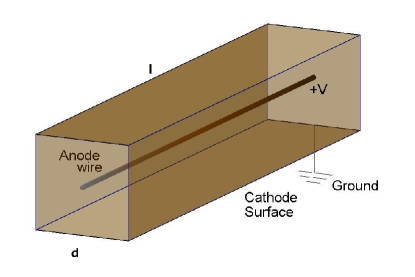
Figure 2: Schematic representation of the wire chamber. The length and the width of the square tube are represented by $l$ and $d$ respectively. The anode wire along its axis has diameter $2a$. The wire is supplied a voltage $+V$ and the cathode is kept grounded.

Several cases for altered tube cross section ($d\times d$), aspect ratio ($\lambda=\frac{l}{d}$) as well as two different wire models have been studied. It should be noted here that if only the mid-plane estimates of the wire chamber are of importance, the computation time can be reduced drastically by using even one element in the axial direction resulting into less than $100$ slender elements in total for the present problem. This has been the case when the computation has been carried out for the mid-plane properties of large aspect ratio chambers. On the other hand, for proper three dimensional computation, the four flat rectangular surfaces have been segmented in to $21$ elements along the $X$-direction and $21$ in $Z$-direction. The anode wire when considered as a polygon has been modeled with $32$ surfaces. The size of influence matrix has varied from $85\times 85$ to $2436\times 2436$ depending upon the scheme of segmentation.

4 Results

The NEBEM calculations for potential and normal electrostatic field ($Y$-component) at the mid-plane of the chamber have been compared with the analytic estimates of an infinitely long tube provided by the Garfield code [11] to demonstrate the accuracy of the solver. In Fig.3 and Fig.4, the results are shown for a variation in the tube cross-section from $5$mm $\times 5$mm to $16$mm $\times 16$mm with wire diameter $50\mu$m, the wire being modeled as a polygon with $32$ surfaces. The aspect ratio, $\lambda=\frac{l}{d}$, has been kept $10$ to retain the property of infiniteness so as to compare with analytic estimates of an infinitely long tube. The comparison of two calculations with a spatial frequency of $100\mu$m shows an excellent agreement over the whole range of tube dimensions. The NEBEM results calculated with thin-wire approximation has not been included in these figures which also yield similar agreement with the analytic ones.

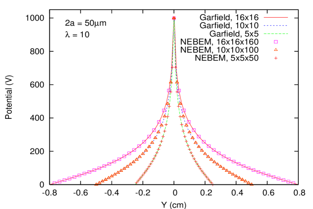
Figure 3: Comparison of potential at the mid-plane of the chamber with aspect ratio $10$ and wire diameter $50\mu$m. Three variations in the chamber cross-section are illustrated along with analytic values.

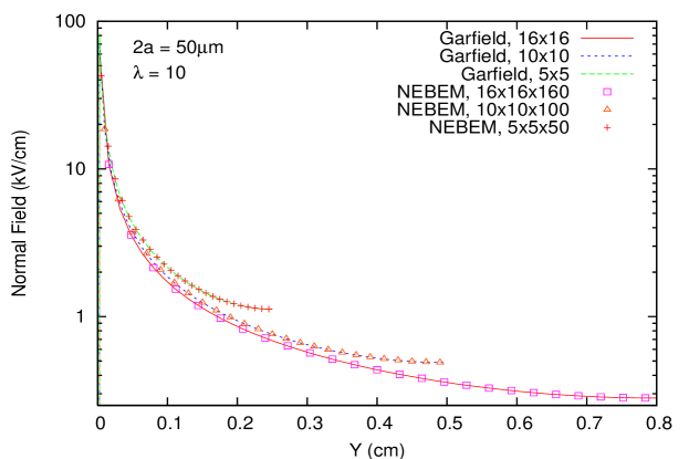
Figure 4: Comparison of normal electric field at the mid-plane of the chamber with aspect ratio $10$ and wire diameter $50\mu$m. Three cases of varied cross-sections are illustrated along with analytic estimates.

The difference of the NEBEM calculations from the analytic values have been estimated as follows.

$$RelativeDeviation(\%)=\frac{Garfield-NEBEM}{Garfield}\times 100$$ (15)

This has been illustrated in Fig.5 by plotting the relative deviation of NEBEM normal electrostatic field from the analytic values calculated at the mid plane of the chamber. The relative deviations estimated with thin-wire approximation have been plotted as well. Since the NEBEM is a full-fledged three dimensional solver, the effect of $\lambda$ of the tube on the field configuration can be studied using it. Several such estimates of relative deviations for different aspect ratios have been shown in Fig.5 calculated using both of polygon with $32$ surfaces and thin-wire models. The cross-section of the tube has been considered to be $10$mm $\times 10$mm with wire diameter $50\mu$m. It has been observed that the departure from the analytic solutions for an infinitely long tube becomes significant when $\lambda$ is reduced to $2$ and below. It becomes apparent (close to $1\%$) as $\lambda$ is dropped down to $2$ and enhances up to $10\%$ when $\lambda$ is still reduced to $1$. The amount of relative deviation in the vicinity of the anode wire is maximum $2\%$ for the smallest aspect ratio. The trend is similar in both of polygon and thin-wire models as can be seen in the figure.

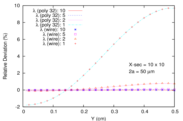
Figure 5: Relative deviation of normal electric field from the analytic values at the mid-plane of the chamber with varied aspect ratios for polygon and thin-wire modeling of the wire. The cross-section of the chamber and the diameter of the wire are $10$mm $\times 10$mm and $50\mu$m respectively.

It should be noted here that the use of end plates is expected to alter the relative deviation particularly at smaller aspect ratios.

The most essential study in such wire chambers is the field configuration in the amplification region which matters most in their performance. Since NEBEM can evaluate three dimensional field at any point in the physical volume including the near-field region, a thorough study of the field values in the amplification region can be made using it. A comparative study has been carried out within twice the diameter from the wire-axis (i.e. $100\mu$m), the closest limit being just $1\mu$m away from the surface of the wire (i.e. $26\mu$m) using two different wire models. The calculations have been shown in Fig.6 for the cases illustrated in Fig.5.

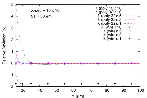
Figure 6: Relative deviation in normal field from the analytic values at close proximity to the anode wire. The tube cross-section and wire diameter are $10$mm $\times 10$mm and $50\mu$m respectively.

Although the agreement between the polygon and thin-wire model is excellent up to quite close proximity of the wire, a departure has been observed within one radius to the wire in case of polygon modeling. It has been observed that the departure is almost negligible (below $1\%$) when larger number of surfaces (about $32$) has been incorporated. It can increase to as high as $5\%$ when less number of surfaces like $12$ is used. It is obvious from the calculation that the thin-wire approximation is adequate to estimate the field configuration in the near-field region in symmetric configurations. However, depending upon the nature of the problem, the polygon model may be useful in calculation of azimuthal variation of properties in an asymmetric configuration. In that case, a modest number of the polygon surfaces should be enough to obtain the field configuration with high accuracy.

Finally, the variation of normal electrostatic field along the axial direction of the tube has been studied which has been plotted in Fig.7. The tube dimension has been considered to be $10$mm $\times 10$mm $\times 100$mm with wire diameter $50\mu$m. The calculations have been carried out at three different transverse locations as indicated in the figure. The middle line represents the calculation done at halfway between the anode and the cathode. The two dimensional analytic solutions provided by the Garfield code have been illustrated in three dimension by the lines representing the uniform field configuration throughout the length. The NEBEM results reproduce the two dimensional analytic values for more than $85\%$ of the tube length. However, in the remaining $15\%$ towards the ends, the three dimensional effects are non-negligible. Even more important point to be noted here is that the NEBEM calculation produces perfectly smooth variation of the field with a spatial frequency of $10\mu$m only while significant fluctuations are known to be present in FDM, FEM and usual BEM solvers because of their strong dependence on nodal properties. This remarkable feature of the present solver should allow more realistic estimation of the electrostatic field of various gas detectors resulting into better gain estimations.

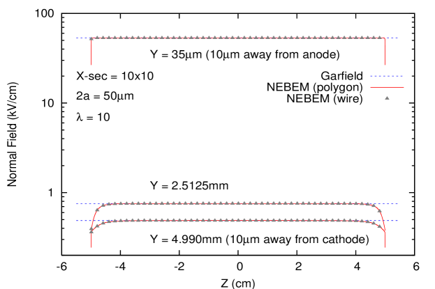
Figure 7: Axial deviation of normal electric field at the mid-plane of the chamber with cross-section $10$mm $\times 10$mm, aspect ratio $10$ and wire diameter $50\mu$m, calculated at three $Y$-positions. Two different wire models are considered.

5 Conclusion

The three dimensional NEBEM solver has yielded accurate electrostatic field configuration of a square tube wire chamber which represents the analytic estimates quite well in most of the detector volume when the aspect ratio is large enough ($\lambda>5$) except at the ends of the chamber where end effects can be observed. For smaller aspect ratios ($\lambda<2$), non-negligible departures (about $2\%$) from the analytic values estimated for infinitely long chamber have been observed even in the amplification region. A large deviation (about $10\%$) has also been observed near the cathode surface. The near-field calculation in the close vicinity to the anode wire (within one diameter) has produced a difference in the results obtained with polygon and thin-wire models. The observation has implied that in order to obtain accurate field estimates with polygon modeling in the asymmetric configuration, an adequate number (e.g.$32$ for error $<1\%$) of polygon surfaces are required to reproduce thin-wire results. The simple but robust formulation of the solver using closed form expressions can also be used to solve for gas detectors of other geometries. Since the solver can produce very smooth and precise estimate of three dimensional electrostatic field even in the near-field region, it should be very useful in providing important information related to the design and interpretation aspects of a wire chamber.

6 Acknowledgement

The authors are thankful to Prof. B. Sinha, Director, SINP, and Prof. S. Bhattacharya, Head, NAP Division of SINP for their encouragement and support throughout this work.

References

- [1] G. A. Erskine, Nuclear Instrumentation and Methods 105 (1972) 565.
- [2] R. Veenhof, Nuclear Instruments and Methods in Physics Research A 419 (1998) 726.
- [3] W. I. Buchanan and N. K. Gupta, Advances in Engineering Software 23 (1995) 111.
- [4] T. M. Lopez and A. Sharma, CERN/IT/99/5 7 (1997).
- [5] S. Mukhopadhyay and N. Majumdar, IEEE Transactions on Nuclear Science 53, No.2 (2006) (to be published)
- [6] A. Renau, F. H. Read and J. N. H. Brunt, Journal of Physics E: Science Instruments 15 (1982) 347.
- [7] S. Mukhopadhyay and N. Majumdar, Advances in Computational and Experimental Engineering and Sciences TechScience Press, 2005
- [8] S. Mukhopadhyay and N. Majumdar, Engineering Analysis with Boundary Elements (accepted)
- [9] M. R. Convery et al., Nuclear Instruments & Methods in Physics Research A 556 (2006) 134.
- [10] B. Van de Vyver, em CERN-THESIS-2002-024 (2002)
- [11] http://garfield.web.cern.ch/garfield