The critical Reynolds number of a laminar mixing layer

Abstract

It has hitherto been widely considered that a mixing layer is unstable at all Reynolds numbers. However this is untenable from energy considerations, which demand that there must exist a non-zero Reynolds number below which disturbances cannot extract energy from the mean flow. It is shown here that a linear stability analysis of similarity solutions of the plane mixing layer, including the effects of flow non-parallelism, using the minimal composite theory and the properties of adjoints following Govindarajan & Narasimha (2005), resolves the issue by yielding non-zero critical Reynolds numbers for coflowing streams of any velocity ratio. The critical Reynolds number so found, based on the vorticity thickness and the velocity differential as scales, varies in the narrow range of $59$ to $55$ as the velocity ratio goes from zero to unity.

1 Introduction

The motivation for the present work arises from an analysis of the stability of a mixing layer due to Betchov & Szewczyk (1963). This analysis, based on the Orr–Sommerfeld (OS) equation, showed that the neutral curve in the wave-number ($\alpha$) – Reynolds number (Re) plane approaches the origin $\alpha=0$ as Re goes to $0$, leading the authors to conclude “No minimum [i.e. critical] Reynolds number is found” for the flow. Mixing layers have been studied extensively since, and recent texts, e.g. Huerre & Rossi (1998, pp. 81–294), Criminale et al. (2003, p. 90) and Drazin & Reid (2004, p. 199–201), still report the critical Reynolds number as zero. This is intriguing, for several early studies of stability (e.g. Prandtl (1935, pp. 178–183), Lin (1955, pp. 31–32, 59+), going back to the two-dimensional analysis of Lorentz (1907, pp. 43–71)), show that (under certain reasonable conditions) a two-dimensional incompressible viscous flow must be stable at sufficiently low Reynolds numbers. Astonishingly, however, there is no analysis in the extensive literature on hydrodynamic stability that yields a non-zero value for this critical Reynolds number. The mixing layer being a very basic flow type, the absence of any definitive commentary on the above issue has led other studies of flows modelled on the mixing layer (e.g.  Solomon, Holloway & Swinney, 1993; Östekin, Cumbo & Liakopoulos, 1999) to base their analyses on the assumption that the critical Reynolds number is zero.

Now all analyses of mixing layer stability, from Esch (1957) to Balsa (1987), start with the OS equation, which is valid only for strictly parallel flow. However, the width of a laminar mixing layer scales as $x^{1/2}$ (where $x$ is the streamwise distance), so the rate of change of thickness (and hence also any parameter measuring the degree of flow non-parallelism) becomes infinite in the limit of $x$ (equivalently Re) going to $0$. In other words, existing studies are based on the assumption of no non-parallelism in a situation where any measure of non-parallelism would be infinite. Thus flow non-parallelism may be expected to play a crucial role in determining the stability characteristics in the limit. Though Bun & Criminale (1994) note that “with viscous effects, the basic flow should be treated as non-parallel”, and other texts (e.g.  Drazin & Reid, 2004, p.197) emphasize that “at small values of Reynolds number the parallel-flow assumption is of questionable validity”, no investigation accounts for the non-parallelism. We show here that a consistent non-parallel flow theory yields finite, non-zero critical Reynolds numbers based on vorticity thickness and velocity differential in the range $55$ to $59$ depending on the velocity ratio.

In a departure from earlier work, the similarity solution of the laminar mixing layer is used as the base flow everywhere in the present analysis. The earlier studies, beginning with ones that assumed zero viscosity, have moved from the discontinuous profile due to Helmholtz to the hyperbolic tangent profile considered by Betchov & Szewczyk (1963). Examples of other approximations appear in Esch (1957), and all later studies to our knowledge use one of these. The similarity profile is a better approximation of reality than any of the above, and its use through what we have called minimal composite theory is both appropriate and convenient in the present approach.

The rest of the paper is arranged as follows. In § 2 the similarity solution of the mean flow profile is presented and some remarks follow. The stability problem is posed and the method of solution briefly outlined in § 3, essentially following the approach used for boundary layers by Govindarajan & Narasimha (1997, 2005). In § 4, the results of the stability analysis are presented and compared with earlier work.

2 Similarity solution of the basic flow

A plane incompressible mixing layer that develops in the positive $x$-direction is considered. The two free-streams flow with velocities $U_{\infty}$ and $\lambda U_{\infty}$ (with $\lambda<1$) before coming into contact with each other at the origin ($x=0$). Both streams are semi-infinite in their lateral ($y$) extent. We omit the case of counterflowing streams ($\lambda<0$) from the present discussion, since they are not relevant to the non-parallel flow theories. Since no other external length scale is present in the problem as formulated, after a sufficient distance from the origin similarity may be taken to be valid.

Henceforth all variables subscripted by d are dimensional quantities. The streamwise coordinate and the coordinate in the direction normal to the flow are $x_{d}$ and $y_{d}$ respectively, and $\nu$ is the kinematic viscosity. The similarity analysis here differs from Schlichting & Gersten (2004, pp. 175–176) only in the definition of the length scale $l_{d}$ in the direction normal to the flow,

$$l_{d}(x_{d})\equiv\displaystyle\sqrt{\nu x_{d}\over U_{\infty}}.$$ (1)

The streamfunction is defined as

$$\mathit{\Phi}_{d}(x_{d},y_{d})=U_{\infty}l_{d}(x_{d})\mathit{\Phi}(y),$$

$y=y_{d}/l_{d}$ being the similarity coordinate. The momentum equation in terms of the non-dimensional streamfunction $\mathit{\Phi}$ becomes

$$\mathit{\Phi}^{\prime\prime\prime}+{1\over 2}\mathit{\Phi}\mathit{\Phi}^{\prime\prime}=0,$$ (2)

where the primes denote derivatives taken with respect to $y$. The boundary conditions to be satisfied are

$$\left.\begin{array}[]{ll}\mathit{\Phi}^{\prime}(y=+\infty)=1,\\[8.0pt] \mathit{\Phi}^{\prime}(y=-\infty)=\lambda\qquad\mbox{ and}\\[8.0pt] \left.(y\mathit{\Phi}^{\prime}-\mathit{\Phi})\right]_{y=\infty}+\lambda\left.(y\mathit{\Phi}^{\prime}-\mathit{\Phi})\right]_{y=-\infty}=0.\end{array}\right\}$$ (3)

The third boundary condition has been a subject of some controversy. As formulated above, it is derived from matching the pressure across the mixing region, following Ting (1959). The zero net transverse force condition suggested by von Karman (1921) results in an identical third boundary condition. Klemp & Acrivos (1972) pointed out an inconsistency in the above formulation and showed that this condition is still incomplete, and further that it cannot be resolved within the context of classical boundary layer theory. Using a different approach to formulate asymptotic expansions to solutions of the Navier–Stokes equations, Alston & Cohen (1992) have however argued that this condition remains the best option compared to the other alternatives used in the literature.

The velocity profiles obtained for different values of $\lambda$ are shown in figure 1. Apart from the displacement of the dividing streamline in the negative $y$ direction, these solutions are identical to those obtained first by Lock (1951). The result for the half jet, i.e. for $\lambda=0$, was validated against that given in Schlichting & Gersten (2004, pp. 175–176). A suitably transformed hyperbolic tangent function is superimposed on the similarity profile for $\lambda=0$ for comparison.

Figure 1: Streamwise velocity profiles from the solution of (2) for different velocity ratios. Solid line, similarity profile for $\lambda=0$; circles, ${1\over 2}(1+\tanh\{2(y+1)/5\})$; dash-dotted line, similarity profile for $\lambda=0.5$; short dashes, similarity profile for $\lambda=0.75$.

Note that for every flow configuration with a $\lambda$ in the range $0$ to $1$, there corresponds an identical but vertically flipped flow with velocity ratio $1/\lambda$. So it is expected that the similarity solution becomes increasingly symmetric about the $x$ axis as $\lambda$ approaches $1$. In the limit $\lambda\rightarrow 1$, redefining the non-dimensional streamfunction as

$$\mathit{\Phi}(y)\equiv(1-\lambda)f(y)+y,$$

the similarity equation (2) becomes

$$f^{\prime\prime\prime}+{1\over 2}[y+(1-\lambda)f]f^{\prime\prime}=0,$$ (4)

with appropriately transformed boundary conditions. Writing ($1-\lambda$) as a small parameter $\epsilon$ and assuming a solution in the form of an asymptotic series in powers of $\epsilon$,

$$f=f_{0}+\epsilon f_{1}+\epsilon^{2}f_{2}+\mbox{ (higher order terms)},$$

we get the streamwise velocity correct to second order in $\epsilon$ as

$$U_{d0}(x_{d},y_{d})=U_{\infty}[1+\epsilon f_{0}^{\prime}(y)]=U_{\infty}\biggl{\{}1-{\epsilon\over 2}\biggl{(}1-\mbox{erf}(y/2)\biggr{)}\biggr{\}}+O(\epsilon^{2}).$$

While such analytically expressible profiles are ubiquitous in the literature, our purpose is to demonstrate that the similarity solution smoothly merges into the error-function profile for $\lambda$ close to $1$. It is therefore not expected (as we shall confirm shortly) that the stability characteristics change very much between these choices. This puts into perspective one of the nuances of our analysis that is different from existing ones, for it must be emphasized that the marked deviation observed in the final result is not to be attributed to the differences in the assumed velocity profiles but to the non-parallel flow analysis.

3 The non-parallel stability problem

A brief outline of the minimal composite theory is described in what follows. A review of the method can be found in Narasimha & Govindarajan (2000).

Each flow quantity, for example the streamfunction, is expressed as the sum of a mean $\mathit{\Phi}_{d}$ and a perturbation ${\hat{\phi\mkern 4.0mu}\mkern-4.0mu}{}_{d}$, where

$$\mathit{\Phi}_{d}(x_{d},y_{d}) = U_{\infty}l_{d}(x_{d})\mathit{\Phi}(y)\qquad\mbox{ and}$$ (5)

$${\hat{\phi\mkern 4.0mu}\mkern-4.0mu}{}_{d}(x_{d},y_{d}) = U_{\infty}l_{d}(x_{d})\phi(x,y)\exp\biggl{[}\mathrm{i}\biggl{(}\int\alpha(x)\mathrm{d}x-\omega t\biggr{)}\biggr{]},$$ (6)

with the (complex) phase speed of the disturbance $c=\omega/\alpha$. Inserting these into the Navier–Stokes equations for two-dimensional incompressible flow written in terms of the streamfunction, and retaining all terms nominally upto $O(\mbox{{Re}}^{-1})$, the non-parallel stability equation can be written as

$$\mathcal{N}\{\phi\}=0,\qquad\mbox{ with boundary conditions}\quad\phi,\mathrm{D}\phi\rightarrow 0\quad\mbox{ at }y=\pm\infty,$$ (7)

where, for the mixing layer,

$$\mathcal{N} \equiv (\mathit{\Phi}^{\prime}-c)(\mathrm{D}^{2}-\alpha^{2})-\mathit{\Phi}^{\prime\prime\prime}+\frac{\mathrm{i}}{\alpha\mbox{{Re}}}\biggl{\{}\mathrm{D}^{4}-2\alpha^{2}\mathrm{D}^{2}+\alpha^{4}+p\mathit{\Phi}\mathrm{D}^{3}\biggr{.}$$

$$+p(\mathit{\Phi}^{\prime}\mathrm{D}^{2}+\mathit{\Phi}^{\prime\prime}\mathrm{D})-\alpha^{2}[2py(\mathit{\Phi}^{\prime}-c)+p\mathit{\Phi}]\mathrm{D}-p\alpha^{2}c+p\mathit{\Phi}^{\prime\prime\prime}$$

$$\biggl{.}+(3\mathit{\Phi}^{\prime}-c)\mbox{{Re}}\alpha\alpha^{\prime}+[\mathit{\Phi}^{\prime\prime\prime}+\alpha^{2}(3\mathit{\Phi}^{\prime}-2c)-\mathit{\Phi}^{\prime}\mathrm{D}^{2}]\mbox{{Re}}\frac{\partial}{\partial x}\biggr{\}},$$

$\mathrm{D}$ is the derivative with respect to $y$ and $p\equiv\mbox{{Re}}(\mathrm{d}l_{d}/\mathrm{d}x_{d})=1/2$. The Reynolds number is based on $U_{\infty}$ and $l_{d}$. Note that in the minimal composite theory the operator $\mathcal{N}$ is flow-specific, and so is different e.g. from that for the boundary layer (see below). Following Govindarajan & Narasimha (1997) the non-parallel operator $\mathcal{N}$ is expressed as the sum of an operator $\mathcal{M}$ that contains all the lowest order terms and an operator $\mathcal{H}$ comprising the higher order terms,

$$\mathcal{M} \equiv (\mathit{\Phi}^{\prime}-c)(\mathrm{D}^{2}-\alpha^{2})-\mathit{\Phi}^{\prime\prime\prime}+\frac{\mathrm{i}}{\alpha\mbox{{Re}}}\mathrm{D}^{4},$$

$$\mathcal{H} \equiv \frac{1}{\mbox{{Re}}}\biggl{\{}p\mathit{\Phi}\mathrm{D}^{3}-2\alpha^{2}\mathrm{D}^{2}+\alpha^{4}+p(\mathit{\Phi}^{\prime}\mathrm{D}^{2}+\mathit{\Phi}^{\prime\prime}\mathrm{D})-\alpha^{2}[2py(\mathit{\Phi}^{\prime}-c)+p\mathit{\Phi}]\mathrm{D}$$

$$-p\alpha^{2}c+p\mathit{\Phi}^{\prime\prime\prime}\biggr{\}}+(3\mathit{\Phi}^{\prime}-c)\alpha\alpha^{\prime}+\mathcal{S}\frac{\partial}{\partial x},$$

$$\mbox{where }\;\qquad\mathcal{S} \equiv [\mathit{\Phi}^{\prime\prime\prime}+\alpha^{2}(3\mathit{\Phi}^{\prime}-2c)-\mathit{\Phi}^{\prime}\mathrm{D}^{2}].$$

The relative order of magnitude of each individual term varies with $y$ because of the presence of the critical layer at $\mathit{\Phi}^{\prime}=c$. While constructing the minimal composite equation that yields results correct upto $O(\mbox{{Re}}^{-1})$, the order of magnitude of any term within the $y$-domain is considered. The final equation consists of all terms that are at least $O(\mbox{{Re}}^{-1})$ somewhere, and rejects all that are $o(\mbox{{Re}}^{-1})$ everywhere in the domain. It must be emphasized that the above equations are different from those in Govindarajan & Narasimha (2005), which were formulated for a boundary layer. For instance, in the construction of the operator $\mathcal{M}$ for the present case clearly no wall layer considerations are needed. Furthermore, the term $p\mathit{\Phi}\mathrm{D}^{3}$, being of higher order everywhere in the mixing layer, is in the operator $\mathcal{H}$, whereas in the boundary layer it is part of $\mathcal{M}$. The solution procedure for estimating the growth of the disturbance, though, remains the same, and is given in that paper in detail. For reference, we recapitulate some of its essential points below.

It is instructive to note that though the non-parallel operator has partial derivatives in both $x$ and $y$, the lowest order terms (comprising $\mathcal{M}$) contain derivatives only in $y$. Taking this as a cue, the total solution $\phi$ is expressed in two parts,

$$\phi(x,y)=A(x)\phi_{m}(x,y)+\epsilon\phi_{h}(x,y).$$ (8)

Here $A(x)$ is the amplitude function that captures the streamwise variation of the lowest order solution $\phi_{m}$, which satisfies the equation

$$\mathcal{M}\{\phi_{m}\}=0.$$ (9)

We consider the downstream growth of disturbances at a constant value of the similarity variable $y$. For future reference, we also define a complex effective wavenumber associated with the non-dimensional streamwise disturbance velocity ${\hat{u\mkern 2.0mu}\mkern-2.0mu}{}$ as

$$\alpha_{\rm{eff}}=\alpha-\mathrm{i}\biggl{(}{1\over A}{\mathrm{d}A\over\mathrm{d}x}+{1\over\partial\phi_{m}/\partial y}{\partial(\partial\phi_{m}/\partial y)\over\partial x}\biggr{)},$$ (10)

such that the growth rate $g$ of ${\hat{u\mkern 2.0mu}\mkern-2.0mu}{}$ is given by

$$g\equiv-\mbox{Im}(\alpha_{\rm{eff}})=-\alpha_{i}+\mbox{Re}\biggl{(}{1\over A}{\mathrm{d}A\over\mathrm{d}x}+{1\over\partial\phi_{m}/\partial y}{\partial(\partial\phi_{m}/\partial y)\over\partial x}\biggr{)},$$ (11)

where $\alpha_{i}$ is the imaginary part of the full complex wavenumber $\alpha$. We find that, in general, a disturbance may amplify at one $y$ and decay at another. Moreover, one disturbance quantity could be amplifying while others decay. The derivative of $\phi_{m}$ with respect to $x$ is obtained by solving (9) for a nearby Re and noting that $\partial/\partial x=p\partial/\partial\mbox{{Re}}$. Substituting from (8) into (7), and noting that $\mathcal{N}=\mathcal{M}+\mathcal{H}$, we obtain the amplitude evolution equation

$$A\mathcal{H}\phi_{m}+{\mathrm{d}A\over\mathrm{d}x}\mathcal{S}\phi_{m}=-\epsilon\mathcal{M}\phi_{h},$$ (12)

the truncated terms here being $O(\mbox{{Re}}^{-2/3})$ compared to the largest of the retained terms. Further the expression for the adjoint of the operator $\mathcal{M}$ is found to be

$$\mathcal{\overline{M}}=(\mathit{\Phi}^{\prime}-c^{*})(\mathrm{D}^{2}-\alpha^{*2})+2\mathit{\Phi}^{\prime\prime}\mathrm{D}-{\mathrm{i}\over\alpha^{*}\mbox{{Re}}}\mathrm{D}^{4}+O(\mbox{{Re}}^{-2/3}),$$

where a quantity superscripted with an asterisk represents its complex conjugate. Using the property of adjoints (cf. Govindarajan & Narasimha, 2005), the contribution to the growth $g$ due to change in the amplitude function, i.e. the quantity $(1/A)\mathrm{d}A/\mathrm{d}x$, is calculated without the need to specifically compute the higher order solution $\phi_{h}$. Equation (12) therefore reduces to

$$A\int_{-\infty}^{\infty}\chi^{*}\mathcal{H}\{\phi_{m}\}\mathrm{d}y+{\mathrm{d}A\over\mathrm{d}x}\int_{-\infty}^{\infty}\chi^{*}\mathcal{S}\{\phi_{m}\}\mathrm{d}y=\mbox{ (higher order terms)},$$

where $\chi$ is the solution of the adjoint problem,

$$\mathcal{\overline{M}}\{\chi\}=0.$$

Now $A\sim O(1)$ and $\mathrm{d}A/\mathrm{d}x$ is $O(\mbox{{Re}}^{-1})$, so the error in the estimation of the growth rate will be $o(\mbox{{Re}}^{-1})$. But as we integrate over a large streamwise distance of $O(\mbox{{Re}})$, the error in the amplitude is expected to be $o(1)$. Here, a solution of the partial differential equation (7) to the desired order of accuracy has been obtained by solving a parametric ordinary differential equation and using the property of adjoints. An obvious advantage is that the complexity of the problem is significantly reduced when compared to the exercise of solving it as a full partial differential equation.

4 Results

4.1 Accuracy of results

Both the parallel and non-parallel stability analyses involve solving an eigenvalue problem. The conditions at infinity are posed at distances sufficiently far away to ensure that results are independent of the size of the domain. For example, on the curve of marginal stability, the Reynolds number for a given $\alpha$ is required to be identical up to the fifth decimal place before any further increase in domain size is considered unnecessary. We notice that at large $y$, $\mathit{\Phi}^{\prime\prime\prime}$ vanishes and the higher derivatives of the eigenfunction with respect to $y$ (appearing in the viscous term) become smaller. Therefore, as an estimate, the eigenfunction decays as $\exp(\pm\alpha y)$, i.e. its $e$-folding rate depends on the wavenumber of the disturbance. The $y$-domain thus needs to be larger for smaller wavenumbers. Further, since the eigenfunctions are discretized as eigenvectors, a sufficient number of grid-points must be contained in the domain so that the results are independent of resolution.

Now, an increase in the number of grid-points directly increases the size of the matrices involved in the eigenvalue problem and this affects the computational effort adversely. For non-dimensional wavenumbers larger than $0.2$, we impose outer boundary conditions at $y=\pm 20$ and use $81$ grid-points with a $\sinh$ grid-stretching. For the smallest wavenumbers considered ($\alpha\simeq 0.02$) the conditions at infinity are imposed at $y=\pm 300$ with $150$ grid-points. Intermediate values were taken to expedite the solution process whenever this did not affect the accuracy above a tolerance level of five significant digits. There is thus a lower cut-off for the real part of the wavenumber in our results, beyond which obtaining numerically accurate results becomes prohibitively expensive computationally. The neutral boundary is defined where the imaginary part of the eigenvalue $\omega$ and the growth rate $g$ are smaller than $1\times 10^{-8}$ and $1\times 10^{-6}$ in magnitude respectively. In calculating the streamwise derivatives, nearby stations are taken corresponding to values of Reynolds number Re apart by $1\%$ of the value at either of these points. Independence of the curve of marginal stability to small deviations in the numerical value of this parameter has also been confirmed.

4.2 Parallel vs. non-parallel analysis

As mentioned before, the non-parallel approach is expected to deviate significantly from the parallel approach in the region where the Reynolds number based on streamwise distance is small.

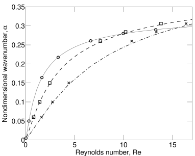
Figure 2: Results of OS (parallel) analysis: circles, Betchov & Szewczyk (1963); solid line, present analysis on $\tanh$ profile; squares, transformed $\tanh$ profile with $\lambda=0$; short dashes, similarity profile with $\lambda=0$; crosses, transformed $\tanh$ profile with $\lambda=0.5$; dash-dot line, similarity profile with $\lambda=0.5$.

First, as validation of the OS solver used, we compare the results of the present analysis on the hyperbolic tangent profile (the case of counterflowing streams with $\lambda=-1$) with those of Betchov & Szewczyk (1963) in figure 2. Secondly, we establish that the result showing the flow to be unstable at $\mbox{{Re}}=0$ is not specific to a counterflow situation, rather it is inherent in the parallel flow assumption. Curves of marginal stability from a parallel analysis on the similarity profiles for the velocity ratios $0$ and $0.5$ are also plotted in figure 2. These are compared with those from a parallel analysis on a suitably transformed hyperbolic tangent profile.

Note that while the similarity solution has a well-defined length scale (1) associated with it, the hyperbolic tangent profile may be arbitrarily scaled. For the results shown in figure 2, the hyperbolic tangent function used is so transformed that its vorticity thickness (14) is identical to that of the similarity solution for the corresponding velocity ratio. We note that all the curves approach the origin, irrespective of whether the hyperbolic tangent or the similarity profile is used.

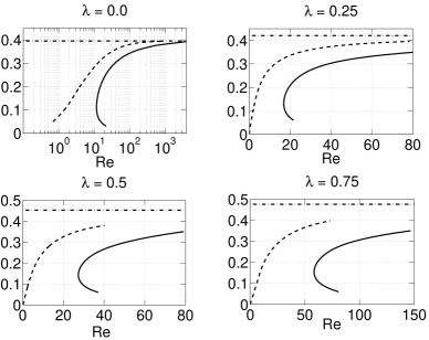
Figure 3: Comparison of the parallel and non-parallel analyses. The Reynolds number is plotted on the horizontal axis. The vertical axis corresponds to the real parts of the wavenumber $\alpha$ and the effective wavenumber $\alpha_{\rm{eff}}$ for the parallel and non-parallel analyses respectively. Short dashes, OS; solid line, non-parallel; dash-dot line, Rayleigh.

Next, the results of the parallel and non-parallel analyses are compared in figure 3 for the four velocity ratios $0.0,0.25,0.5$ and $0.75$. The results correspond to the respective similarity profiles. The relevant quantity on the vertical axis for the results of the parallel analysis is the physical wavenumber $\alpha$, whereas for the non-parallel analysis it is the real part of the effective wavenumber $\alpha_{\rm{eff}}$ defined in (10).

Apart from the terms already present in the OS equation, the non-parallel operator $\mathcal{N}$ includes further terms that essentially provide a correction at low Re. It is expected that the difference between the parallel and non-parallel approaches diminishes in the limit Re $\rightarrow\infty$. Figure 3 shows that the curves of marginal stability, from both parallel and non-parallel analyses, do indeed approach the neutrally stable mode of the solution to Rayleigh’s equation for each of the velocity ratios considered above. Note that the curves for $\lambda=0$ have been plotted with Re on a log scale to show that the results are indistinguishable as Re $\rightarrow\infty$; but differences are noticeable even at $\mbox{{Re}}=10^{3}$!

From § 3 it is evident that the curve of marginal stability and hence the critical Reynolds number can vary depending on the $y$ value at which the growth rate $g$ is determined. The monitoring location makes a huge difference to the stability result in the case of boundary layers Govindarajan & Narasimha (1997). But for the present flow the contribution from the last term in $g$ is smooth in $y$. The critical $\mbox{{Re}}^{*}$ (13) was observed to vary within a range that was about $10\%$ of the value of the critical $\mbox{{Re}}^{*}$ at $y=0$ while traversing from $y=-1.0$ to $y=0.5$. We do not expect any widely different behaviour outside this range as the variation in the velocity profile becomes negligible. It is also interesting to note that the minimum of the critical Reynolds numbers for any given velocity ratio seems to occur close to the $y$-location where the streamwise velocity profile has the maximum slope (see figure 1). With $y$ rescaled with respect to the vorticity thickness, for the four velocity ratios considered, the location of minimum critical $\mbox{{Re}}^{*}$ deviates most from the location of maximum slope for $\lambda=0.25$ (by $0.019$ units) and the least for $\lambda=0$ (by $0.001$ units). All the results from the non-parallel analysis presented in this paper correspond to a monitoring location fixed at $y=0$.

4.3 Critical Reynolds numbers

The variation of critical Reynolds number Re with velocity ratio is shown in figure 4. A more appropriate Reynolds number in the present flow would be one defined in terms of the velocity difference and the vorticity thickness,

$$\mbox{{Re}}^{*}\equiv{(1-\lambda)U_{\infty}\delta_{d}\over\nu}={(1-\lambda)^{2}\over\mathit{\Phi^{\prime\prime}_{max}}}\mbox{{Re}}$$ (13)

where $(1-\lambda)U_{\infty}$ is the velocity difference, and

$$\delta_{\omega}(x)\equiv l_{d}(x){(1-\lambda)\over\mathit{\Phi^{\prime\prime}_{max}}}$$ (14)

is the vorticity thickness determined by the maximum slope of the velocity profile, $\mathit{\Phi^{\prime\prime}_{max}}$.

The variation of critical $\mbox{{Re}}^{*}$ with velocity ratio is shown in figure 4. It varies monotonically with $\lambda$ and approaches a finite limiting value of $55.3$ as $\lambda$ goes to $1$. Also, the variation of critical $\mbox{{Re}}^{*}$ with $\lambda$ is found to be much less than the variation in critical Re.

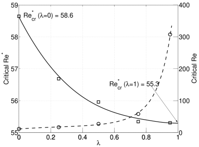
Figure 4: Variation of the critical Reynolds number with velocity ratio. Circles, $\mbox{{Re}}=U_{\infty}l_{d}/\nu$; squares, $\mbox{{Re}}^{*}$ (13). (Dashed and solid curves are fits through the data points.)

5 Conclusions

The main result of the present work is the demonstration of the existence of a non-zero critical Reynolds number for a laminar plane incompressible mixing layer. Choosing the vorticity thickness and velocity differential as length and velocity scales, this critical Reynolds number varies in the narrow range from $58.6$ at $\lambda=0$ to $55.3$ at $\lambda=1$. The present result puts into perspective the prevalent understanding of linear stability of the mixing layer. It also underlines the relevance of a non-parallel analysis vis-a-vis a parallel one in regard to this flow and other open flows exhibiting a high degree of non-parallelism. This is a striking example of a flow where the use of non-parallel theory is essential to avoid drawing incorrect physical conclusions. Though parallel flow theory has given revealing insights to instability mechanisms for over a century, there are regimes of flow where this theory is qualitatively wrong.

The finding of a critical Reynolds number which is not too low has an appealing consequence. The laminar similarity flow analysed here is physically realizable only at some distance downstream of the splitter plate, and the results may therefore be verified experimentally or by direct numerical simulations. This is not possible for the earlier parallel flow results. We note that since the flow is convectively stable below $\mbox{{Re}}^{*}=55$, the question of absolute instability below this Reynolds number does not arise. While it is outside the thrust of the present work, it is relevant to mention that for inviscid flow, from a parallel analysis, it is well established Huerre & Monkewitz (1985) that the instability is convective for any mixing layer formed by coflowing streams.

We also claim that for the purpose of stability analysis, the dependence of results on the exact velocity profile is weak, the form suffices to obtain results to a consistently good accuracy. For all the non-parallel, parallel and inviscid analyses carried out on the similarity profiles, the results differ from corresponding analyses on the (suitably rescaled) hyperbolic tangent profiles by no more than $5\%$. This is in contrast to wall-bounded shear flows where the stability results are very sensitive to the mean-flow velocity profile.