Relativistic calculation of L$\beta_{2}$ satellite spectra of W and Au

Abstract

L$\beta_{2}$ X-ray satellite spectra of tungsten and gold are calculated using the Multi-Configuration Dirac-Fock energies and compared with recent experimental data. New calculations of L₁-L₃M₅ Coster-Kronig transition energies for tungsten are presented, confirming the origin of the L$\beta_{2}$ visible satellites reported by two experimental groups. We found the value 5.09 eV for the average energy of the L₁-L₃M₅ Coster-Kronig transition in tungsten. A detailed calculation of the L$\beta_{2}$ and L$\beta_{15}$ satellite spectra was performed for gold.

1 Introduction

X-ray lines from almost neutral atoms are seldom pure, being in most cases contaminated by the so-called satellite lines, that is, X-ray lines that result from transitions in multi-inner hole atomic configurations. In heavy atoms, X-ray lines resulting from L $\to$ M,N hole transitions with a M spectator hole lead, in general, to satellites that can be resolved from the diagram line (visible satellites), whereas the ones with N-, O- or P-shell spectator holes usually appear embedded within the natural width of the parent line (hidden satellites).

The study of X-ray satellite lines in systems where only one spectator inner hole exists is more than seventy years old, yet not very many works on this subject have been published. Ritchmeyer and Ramberg 1 compared their computed satellite structure of L$\alpha_{1,2}$ (L₃ $\to$ M_4,5 hole transitions), L$\beta_{2}$ (L₃ $\to$ N₅) and L$\beta_{15}$ (L₃ $\to$ N₄) spectra for gold with experimental data. L$\alpha$ X-ray satellite spectra of elements between Zr and Cd were studied by Juslén et al 2 . Doyle and Shafroth 3 measured the intensities of L$\alpha$ and L$\beta_{1}$ (L₂ $\to$ M₄) satellites of elements in the $37\leq Z\leq 56$ region. Hague et al 4 reported on silver L$\alpha$ satellites. Extensive tables of relativistic energies of L X-ray satellite lines, using the Dirac-Fock-Slater (DFS) approach including quantum electrodynamic corrections, were published by Parente et al 5 . The L$\alpha_{1}$ satellite structures of iridium, gold and uranium were studied theoretically by Parente et al 6 and experimentally by Carvalho et al 7 . The possibility that L X-ray satellite lines, not predicted by theory, could be present in tungsten was raised by Salgueiro et al 8 , to explain their experimental data. A simple model to study the relative intensities of satellite and diagram X-ray lines following L-shell ionization in the region around $Z=50$ was proposed by Xu and Rosato 9 . Most recently, Vlaicu et al 10 studied the L emission spectrum of tungsten, confirming the existence of the satellite lines found by Salgueiro et al 8 , and later Oohashi et al 11 focused on the origin of the L$\beta_{2}$ visible satellite lines in gold.

The existence of satellite lines in X-ray spectra has been explained long ago by the creation of multiple vacancies in inner-shells, resulting from the ionization process. Two mechanisms have been proposed for the creation of double vacancies after a primary ionization in the L₁ or L₂ subshells, namely shake-off and L_i-L${}_{j}X_{k}$ Coster-Kronig transitions. Here $i=1,2$, $j=2,3$ (with $i\neq j$), and $X_{k}$ may be any outer subshell. The shake process, for energies not far above the threshold, depends on the excitation energy 12 , whereas Coster-Kronig transitions are independent on the excitation energy. Furthermore, Coster-Kronig transitions are highly probable when energetically allowed so that, in this case, the atom, after the primary ionization, will unavoidably end up with two inner-shell vacancies.

Atomic K- and L-shells relativistic radiationless transition probabilities for 22 elements with atomic numbers $18\leq Z\leq 96$ were published in 1979 by Chen et al 13 . Earlier, in 1977, the same authors had found L₁-L₃M_4,5 Coster-Kronig transitions to be energetically forbidden in the region $50\leq Z\leq 79$ 14 . However, in 1987, Salgueiro et al 8 obtained tungsten L$\alpha$ X-ray spectra where satellite lines were present, which could not be explained by the shake mechanism. Therefore they suggested that, most probably, Coster-Kronig L₁-L₃M₅ transitions could take place in tungsten, contrary to Chen et al predictions. The existence of these satellite lines was confirmed in 1998 by Vlaicu and co-workers 10 . We note, however, that Agarwal 15 already referred the existence of L₁-L₃M₅ Coster-Kronig transitions for $Z>73$ in 1979.

In this work we used the multi-configuration Dirac-Fock code of Desclaux and Indelicato 16 ; 17 ; 17a to calculate the energies of L₁- and L₃M_4,5-hole levels of tungsten, looking for the possibility of existence of L₁-L₃M_4,5 Coster-Kronig transitions. Our results led to the conclusion that L₁-L₃M₅ transitions are indeed energetically allowed in tungsten, contrary to Chen et al 14 prediction. Furthermore, we used the same code to compute transition energies of the X-ray lines in the L$\beta_{2}$ satellite band of tungsten. As the number of lines involved is too big to handle, we used the method suggested by Parente et al 5 , using Racah’s algebra, to predict the shape of this satellite band.

The L$\beta_{2}$ and L$\beta_{15}$ satellite bands of gold, where the number of transitions allows for a full calculation, were also studied in this work and compared with recent experimental results 11 . Spectator holes in all possible subshells were considered in the study, including the ones that give origin to hidden satellites. To assess the accuracy of the method that makes use of Racah’s algebra, we also used this method for gold, to allow for a comparison with the results of the full calculation.

2 Calculation of atomic wave functions and transition probabilities

Bound states wave functions are calculated using the Dirac-Fock program of J. P. Desclaux and P. Indelicato. Details on the Hamiltonian and the processes used to build the wave-functions can be found elsewhere 16 ; 17 ; 18 .

The total wave function is calculated with the help of the variational principle. The total energy of the atomic system is the eigenvalue of the equation

$${\cal H}^{\mbox{{\tiny no pair}}}\Psi_{\Pi,J,M}(\ldots,\bm{r}_{i},\ldots)=E_{\Pi,J,M}\Psi_{\Pi,J,M}(\ldots,\bm{r}_{i},\ldots),$$ (1)

where $\Pi$ is the parity, $J$ is the total angular momentum eigenvalue, and $M$ is the eigenvalue of its projection on the $z$ axis $J_{z}$. The MCDF method is defined by the particular choice of a trial function to solve equation (1) as a linear combination of configuration state functions (CSF):

$$\left|\mathit{\Psi}_{\mathit{\Pi},J,M}\right\rangle=\sum_{\nu=1}^{n}c_{\nu}\left|\nu,\mathit{\Pi},J,M\right\rangle.$$ (2)

The CSF are also eigenfunctions of the parity $\mathit{\Pi}$, the total angular momentum $J^{2}$ and its projection $J_{z}$. The label $\nu$ stands for all other numbers (principal quantum number, …) necessary to define unambiguously the CSF. The $c_{\nu}$ are called the mixing coefficients and are obtained by diagonalization of the Hamiltonian matrix coming from the minimization of the energy in equation (2) with respect to the $c_{\nu}$. The CSF are antisymmetric products of one-electron wave functions expressed as linear combination of Slater determinants of Dirac 4-spinors

$$\left|\nu,\mathit{\Pi},J,M\right\rangle=\sum_{i=1}^{N_{\nu}}d_{i}\left|\begin{array}[c]{ccc}\psi_{1}^{i}\left(r_{1}\right)&\cdots&\psi_{m}^{i}\left(r_{1}\right)\\ \vdots&\ddots&\vdots\\ \psi_{1}^{i}\left(r_{m}\right)&\cdots&\psi_{m}^{i}\left(r_{m}\right)\end{array}\right|.$$ (3)

where the $\psi$-s are the one-electron wave functions and the coefficients $d_{i}$ are determined by requiring that the CSF is an eigenstate of $J^{2}$ and $J_{z}$. The $d_{i}$ coefficients are obtained by requiring that the CSF are eigenstates of $J^{2}$ and $J_{z}.$ A variational principle provides the integro-differential equations to determine the radial wave functions and a Hamiltonian matrix that provides the mixing coefficients $c_{\nu}$ by diagonalization. One-electron radiative corrections (self-energy and vacuum polarization) are added afterwards. All the energies are calculated using the experimental nuclear charge distribution for the nucleus.

The so-called Optimized Levels (OL) method was used to determine the wave function and energy for each state involved. Thus, spin-orbitals in the initial and final states are not orthogonal, since they have been optimized separately. The formalism to take in account the wave functions non-orthogonality in the transition probabilities calculation has been described by Löwdin 19 . The matrix element of a one-electron operator $O$ between two determinants belonging to the initial and final states can be written

$$\left\langle\nu\mathit{\Pi}JM\right|\sum_{i=1}^{N}O\left(r_{i}\right)\left|\nu^{\prime}\mathit{\Pi}^{\prime}J^{\prime}M^{\prime}\right\rangle=$$

$$\times\frac{1}{N!}\left|\begin{array}[c]{ccc}\psi_{1}\left(r_{1}\right)&\cdots&\psi_{m}\left(r_{1}\right)\\ \vdots&\ddots&\vdots\\ \psi_{1}\left(r_{m}\right)&\cdots&\psi_{m}\left(r_{m}\right)\end{array}\right|$$ (7)

$$\times\sum_{i=1}^{m}O\left(r_{i}\right)\left|\begin{array}[c]{ccc}\phi_{1}\left(r_{1}\right)&\cdots&\phi_{m}\left(r_{1}\right)\\ \vdots&\ddots&\vdots\\ \phi_{1}\left(r_{m}\right)&\cdots&\phi_{m}\left(r_{m}\right)\end{array}\right|,$$ (11)

where the $\psi_{i}$ belong to the initial state and the $\phi_{i}$ and primes belong to the final state. If $\psi=\left|n\kappa\mu\right\rangle$ and $\phi=\left|n^{\prime}\kappa^{\prime}\mu^{\prime}\right\rangle$ are orthogonal, i.e., $\left\langle n\kappa\mu|n^{\prime}\kappa^{\prime}\mu^{\prime}\right\rangle=\delta_{n,n^{\prime}}\delta_{\kappa,\kappa^{\prime}}\delta_{\mu,\mu^{\prime}}$, the matrix element (11) reduces to one term $\left\langle\psi_{i}\right|O\left|\phi_{i}\right\rangle$ where $i$ represents the only electron that does not have the same spin-orbital in the initial and final determinants. Since $O$ is a one-electron operator, only one spin-orbital can change, otherwise the matrix element is zero. In contrast, when the orthogonality between initial and final states is not enforced, one gets 19

$$\left\langle\nu\mathit{\Pi}JM\right|\sum_{i=1}^{N}O\left(r_{i}\right)\left|\nu^{\prime}\mathit{\Pi}^{\prime}J^{\prime}M^{\prime}\right\rangle=\sum_{i,j^{\prime}}\left\langle\psi_{i}\right|O\left|\phi_{j^{\prime}}\right\rangle D_{ij^{\prime}},$$ (12)

where $D_{ij^{\prime}}$ is the minor determinant obtained by crossing out the $i$th row and $j^{\prime}$th column from the determinant of dimension $N\times N$, made of all possible overlaps $\left\langle\psi_{k}|\phi_{l^{\prime}}\right\rangle$.

Radiative corrections are also introduced, from a full QED treatment. The one-electron self-energy is evaluated using the one-electron values of Mohr and coworkers 20 ; 21 ; 22 and corrected for finite nuclear size 23 . The self-energy screening and vacuum polarization are treated with an approximate method developed by Indelicato and coworkers 24 ; 25 ; 26 ; 27 .

3 Results

3.1 Tungsten

Using the MCDF code of Desclaux and Indelicato 16 ; 17 , we calculated the energies of all levels in the L₁- and L₃M₅-hole configurations of tungsten, to check for the possibility of Coster-Kronig transitions between these two configurations. Interaction of the inner holes with electrons in outer unfilled shells was taken in account and full relaxation was included but no electronic correlation.

There are 63 energy levels in the L₁ configuration. We found 359 energy levels in the L₃M₅ configuration with energies below the lowest energy level of the L₁ configuration. Thus, we arrive to the conclusion that L₁-L₃M₅ Coster-Kronig transitions are indeed possible in tungsten, originating the double L₃M₅ vacancy state which afterwards yield the satellite lines first detected by Salgueiro et al 8 and confirmed by Vlaicu et al 10 . Averaging over initial and final state energies, we found for the radiationless transition the energy of 5.09 eV.

This value is to be compared to -2.70 eV found by Chen et al 14 , using a relativistic DFS approach. In the latter work coupling with unfilled outer shells was neglected. These authors present the Coster-Kronig transition energies as differences of initial and final average total system energies, which does not allow for a detailed comparison between individual level energies.

Using the MCDF computer code, we calculated the energies of all possible L${}_{3}\to$N₅ radiative transitions in the presence of a M₅ spectator hole, L₃M₅-M₅N₅ transitions, that yield the L$\beta_{2}$ satellite band. In general, to each pair of initial and final angular momenta correspond several X-ray transitions. A full calculation of transition probabilities would be, in this case, a formidable task, due to the enormous number, more than one hundred thousand, of authorized transitions. Instead, we used Racah’s algebra to compute the relative line intensities, using the method of Parente et al 5 . This method assumes:

1. The initial multiplet states are populated statistically;

2. The effect of the multiplet energy differences on the X-ray matrix elements can be neglected;

3. The Auger decay rates of the various multiplet states of a configuration can be taken to be identical. In fact, for heavy atoms there are so many open Auger channels that the multiplet effect on Auger emission rates for double-hole states becomes minimal.

The angular momenta resulting from the unfilled shells are $j_{1},j_{2},j_{3}$ and $j^{\prime}_{1},j^{\prime}_{2},j^{\prime}_{3}$ for the initial and final configurations, respectively, where ${j_{3}}$ and ${j_{3}^{\prime}}$ refer to the outer shell electrons.

Under the above assumptions, the intensity for the line

$\left|~{}j_{1}j_{2}(J_{12}),j_{3};J\right\rangle\to\left|j_{1}^{\prime}j_{2}^{\prime}(J_{12}^{\prime}),~{}j_{3}^{\prime};J^{\prime}\right\rangle$

is found to be proportional to

$$\left|\underset{J_{13}^{\prime}}{\sum}\left(2J_{13}^{\prime}+1\right)\sqrt{\left(2J_{12}^{\prime}+1\right)\left(2J_{12}+1\right)\left(2J^{\prime}+1\right)\left(2J+1\right)}\right.$$

$$\left.\times\sqrt{\left(2j_{1}+1\right)\left(2j_{2}^{\prime}+1\right)}\right.$$

$$\times\left.\left(-1\right)^{J_{12}^{\prime}+j_{3}^{\prime}+3J_{13}^{\prime}+j_{2}^{\prime}+3j_{1}+j_{2}+j_{3}+J^{\prime}+1}\right.$$

$$\left.\times\left\{\begin{array}[c]{ccc}J_{12}^{\prime}&j_{3}^{\prime}&J^{\prime}\\ J_{13}^{\prime}&j_{2}^{\prime}&j_{1}^{\prime}\end{array}\right\}\left\{\begin{array}[c]{ccc}j_{1}&j_{2}&J_{12}\\ j_{3}&J&J_{13}^{\prime}\end{array}\right\}\left\{\begin{array}[c]{ccc}j_{2}^{\prime}&J^{\prime}&J_{13}^{\prime}\\ J&j_{1}&1\end{array}\right\}\right|^{2},$$ (19)

where $J_{ik}$ results from the coupling between angular momenta $j_{i}$ and $j_{k}$. In what concerns the L₃M₅-M₅N₅ transitions, we have $j_{1}=\dfrac{3}{2}$; $j_{2}=j_{2}^{\prime}=\dfrac{5}{2}$; $j_{1}^{\prime}=\dfrac{5}{2}$. For tungsten $j_{3}=0,\ldots,6$; $j_{3}^{\prime}=0,\ldots,6$; $J=0,\ldots,10$; $J^{\prime}=0,\ldots,11$. For each pair of $J,J^{\prime}$ values, the remaining angular momenta values can be found using standard angular momenta calculations. We assumed only one line for each pair of initial and final angular momenta values, assigning to this line the weighted energy and the sum of the line component intensities, in arbitrary units. As L₃M₅-M₅N₄ transition lines are much less intense that L₃M₅-M₅N₅ lines, we did not include them in the calculation for tungsten.

We assume that the natural width of the L₃M₅-M₅N₅ satellite line is given by  14

$$\Gamma\left(\text{L}_{3}\text{M}_{5}\text{-M}_{5}\text{N}_{5}\right)=\Gamma_{\text{L}_{3}}^{\text{tot}}+2\Gamma_{\text{M}_{5}}^{\text{tot}}+\Gamma_{\text{N}_{5}}^{\text{tot}},$$ (20)

where $\Gamma_{X}^{\text{tot}}$ is the natural width of $X$ level. Using the values proposed by Campbell and Papp 30 we obtained 12.2 eV for the width of each of those satellite lines. In this way we arrived at the tungsten L$\beta_{2}$ satellite band presented in figure 1, together with the corresponding spectrum generated using the DFS energy values of Parente et al 5 .

Due to the fact that only the lowest levels of the initial L₃M₅ hole configuration are fed by Coster-Kronig transitions from the L₁ hole initial configuration, the theoretical X-ray satellite band generated in this work is much narrower than if all initial levels were fed. This is clearly shown in figure 1, as the satellite band computed using DFS energy values included all energy levels of the L₃M₅ configuration as initial levels.

This prediction can be compared with the experimental data of Vlaicu et al (figure 2 of  10 ). Although the data resolution is very poor, for obvious lack of statistics, the proeminent peak with energy around 10010 eV is well reproduced in the theoretical band (figure 1 - MCDF). It is obvious that experimental results with better statistics are needed.

Vlaicu et al 10 estimated relative intensities of the L-satellite lines for tungsten, using the expressions proposed by Xu and Rosato 9 , following the model of Krause et al  31 , with values obtained by other authors for the pertinent quantities. As they used Chen et al 14 results for the Coster-Kronig transition probabilities, they assumed that the Coster-Kronig channel for creating M-shell spectator holes is closed, contrary to the findings of the present work.

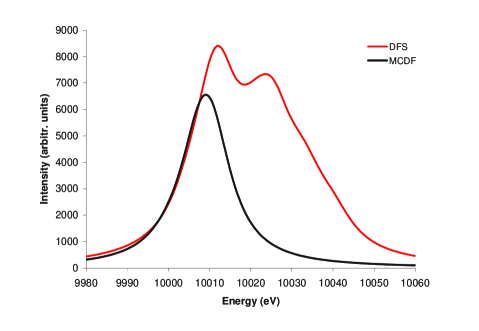
Figure 1: Calculated L$\beta_{2}$ satellite band of tungsten, using Dirac-Fock-Slater - DFS 5 , and Multi-Configuration Dirac-Fock - MCDF (this work) energy values, respectively. In both cases, relative intensities were calculated in the present work using Racah’s algebra, as described in the text. The bands are normalized in intensity.

3.2 Gold

3.2.1 Coster-Kronig transition energies

The L$\beta_{2}$ and L$\beta_{15}$ satellite bands of gold were studied in this work. In this case, the existence of both L₁-L₃M₄ and L₁-L₃M₅ Coster-Kronig transitions were predicted by Chen et al  14 and confirmed by our own calculation.

We found for the L₁-L₃M₄ Coster-Kronig transition in gold the energy of $38.23$ eV and for the L₁-L₃M₅ transition the energy of $132.15$ eV. These values are close to the 37.65 eV and 130.39 eV values, respectively, obtained by Chen et al 13 .

The theoretical L$\beta_{2}$ satellite band of gold was obtained by calculating the transition probabilities for all possible dipolar electric transitions corresponding to the decay of the L₃M₅ and L₃M₄ double-hole configurations, in the energy window between 11600-11700 eV, and, in a separate way, using Racah’s algebra method, as was done for tungsten.

3.2.2 Full MCDF calculation of satellite band

In gold, 8 and 7 energy levels correspond to the L₃M₅- and L₃M₄-hole configurations respectively. On the other hand, 11 and 8 levels correspond to the M₅N₅ and M₄N₅ configurations. This leads to 149 possible electric-dipole allowed lines between the levels of the L₃M_4,5 and M_4,5N₅ configurations that yield the L$\beta_{2}$ visible satellite band. The calculations of the energies and transition probabilities for these lines were performed using the MCDF code of Desclaux and Indelicato, in single-configuration mode, which includes all relativistic CSF originated from a single LS configuration.

Table 1: Energies in eV and transition probabilities ($W$) in s^-1 for gold L$\beta_{2}$, L$\beta_{15}$, and L$\beta_{3}$ diagram lines.

L3 - N5 (L$\beta_{2}$)		L3 - N4 (L$\beta_{15}$)		L1 - M3 (L$\beta_{3}$)
Energy	$W$	Energy	$W$	Energy	$W$
11581.36	1.38$\times 10^{14}$	11563.24	1.28$\times 10^{13}$	11612.24	1.67$\times 10^{14}$
11581.33	1.54$\times 10^{13}$	11563.20	2.66$\times 10^{12}$	11611.82	8.31$\times 10^{13}$
11581.40	2.14$\times 10^{14}$	11563.21	2.55$\times 10^{12}$	11611.87	4.15$\times 10^{14}$
		11563.17	2.28$\times 10^{13}$

Table 2: Energies in eV and transition probabilities ($W$) in s^-1 for gold L$\beta_{2}$ and L$\beta_{15}$ visible satellite lines.

L3M5 - M5N5		L3M4 - M4N5		L3M5 - M5N4		L3M4 - M4N4
Energy	$W$	Energy	$W$	Energy	$W$	Energy	$W$
11627.05	3.38$\times 10^{06}$	11645.44	5.88$\times 10^{11}$	11614.35	4.44$\times 10^{12}$	11616.27	4.51$\times 10^{07}$
11630.44	3.69$\times 10^{11}$	11645.50	1.12$\times 10^{12}$	11614.37	9.63$\times 10^{10}$	11625.33	4.12$\times 10^{12}$
11630.50	1.25$\times 10^{13}$	11645.52	9.47$\times 10^{10}$	11614.41	1.13$\times 10^{11}$	11625.34	2.94$\times 10^{11}$
11631.65	1.28$\times 10^{13}$	11646.48	3.27$\times 10^{08}$	11614.43	3.57$\times 10^{12}$	11625.35	3.04$\times 10^{11}$
11631.71	2.85$\times 10^{11}$	11647.89	9.95$\times 10^{11}$	11615.88	6.82$\times 10^{08}$	11625.35	2.70$\times 10^{12}$
11635.82	1.91$\times 10^{13}$	11647.91	9.18$\times 10^{12}$	11617.83	2.24$\times 10^{12}$	11625.97	1.95$\times 10^{12}$
11635.84	1.34$\times 10^{12}$	11647.94	1.45$\times 10^{13}$	11617.89	1.73$\times 10^{12}$	11625.98	9.88$\times 10^{11}$
11635.90	1.37$\times 10^{12}$	11647.96	8.51$\times 10^{11}$	11617.89	6.45$\times 10^{10}$	11629.82	1.39$\times 10^{08}$
11635.93	1.22$\times 10^{13}$	11650.18	2.27$\times 10^{12}$	11621.86	1.38$\times 10^{12}$	11633.24	2.47$\times 10^{12}$
11638.60	1.16$\times 10^{12}$	11650.20	3.49$\times 10^{13}$	11621.90	2.44$\times 10^{12}$	11633.25	1.27$\times 10^{11}$
11638.66	5.08$\times 10^{13}$	11650.24	4.96$\times 10^{13}$	11621.92	2.86$\times 10^{11}$	11633.26	1.75$\times 10^{12}$
11638.70	6.23$\times 10^{13}$	11653.43	1.53$\times 10^{08}$	11623.20	1.65$\times 10^{08}$	11634.52	2.70$\times 10^{12}$
11639.27	5.04$\times 10^{05}$	11654.39	2.35$\times 10^{12}$	11624.62	2.74$\times 10^{10}$	11634.54	3.13$\times 10^{11}$
11640.46	1.06$\times 10^{12}$	11654.41	6.01$\times 10^{13}$	11624.65	1.72$\times 10^{11}$	11634.55	1.51$\times 10^{12}$
11640.46	1.38$\times 10^{12}$	11654.45	7.81$\times 10^{13}$	11624.65	2.57$\times 10^{11}$	11634.63	2.90$\times 10^{12}$
11640.52	4.36$\times 10^{10}$	11655.15	2.25$\times 10^{12}$	11624.68	1.35$\times 10^{10}$	11634.69	1.43$\times 10^{11}$
11646.62	3.07$\times 10^{12}$	11655.15	4.37$\times 10^{12}$	11626.66	1.25$\times 10^{11}$	11634.71	2.00$\times 10^{12}$
11646.69	5.16$\times 10^{12}$	11655.22	1.14$\times 10^{13}$	11626.66	2.75$\times 10^{12}$	11635.05	1.83$\times 10^{12}$
11646.69	2.86$\times 10^{12}$	11655.23	2.12$\times 10^{12}$	11626.68	1.91$\times 10^{12}$	11635.06	1.95$\times 10^{11}$
11646.71	5.90$\times 10^{11}$	11655.82	4.42$\times 10^{11}$	11633.46	5.46$\times 10^{08}$	11635.06	1.00$\times 10^{12}$
11647.32	3.55$\times 10^{12}$	11655.85	6.54$\times 10^{11}$	11634.69	5.01$\times 10^{12}$	11638.91	6.71$\times 10^{06}$
11647.38	1.72$\times 10^{11}$	11655.87	1.36$\times 10^{10}$	11634.70	1.46$\times 10^{11}$	11642.44	1.14$\times 10^{07}$
11647.46	2.46$\times 10^{12}$	11657.61	3.27$\times 10^{12}$	11634.76	3.81$\times 10^{12}$	11642.54	6.92$\times 10^{12}$
11649.22	1.05$\times 10^{12}$	11657.62	1.74$\times 10^{13}$	11636.15	3.11$\times 10^{12}$	11642.55	3.05$\times 10^{11}$
11649.25	1.49$\times 10^{13}$	11657.67	3.08$\times 10^{13}$	11636.18	2.22$\times 10^{12}$	11642.60	2.61$\times 10^{11}$
11649.29	2.13$\times 10^{13}$	11658.09	4.67$\times 10^{11}$	11636.21	1.80$\times 10^{11}$	11642.62	5.18$\times 10^{12}$
11650.77	1.21$\times 10^{12}$	11658.11	9.65$\times 10^{12}$	11638.16	1.01$\times 10^{11}$	11644.24	9.65$\times 10^{11}$
11650.83	3.16$\times 10^{13}$	11658.15	1.30$\times 10^{13}$	11638.17	2.10$\times 10^{12}$	11644.25	2.05$\times 10^{11}$
11651.99	3.29$\times 10^{13}$	11658.17	5.34$\times 10^{11}$	11638.22	1.57$\times 10^{12}$	11644.26	2.09$\times 10^{11}$
11658.25	1.85$\times 10^{07}$	11659.00	8.31$\times 10^{12}$	11638.22	9.85$\times 10^{10}$	11644.26	4.15$\times 10^{11}$
11658.93	7.78$\times 10^{07}$	11659.07	1.63$\times 10^{13}$	11646.35	9.90$\times 10^{10}$	11644.42	5.92$\times 10^{06}$
11660.33	1.06$\times 10^{13}$	11659.91	6.87$\times 10^{09}$	11646.36	2.29$\times 10^{11}$	11648.09	1.00$\times 10^{12}$
11660.42	1.19$\times 10^{12}$	11661.46	1.57$\times 10^{09}$	11646.41	5.56$\times 10^{11}$	11648.11	4.67$\times 10^{11}$
11660.43	5.88$\times 10^{12}$			11646.42	1.18$\times 10^{11}$
11660.73	6.33$\times 10^{11}$			11649.14	1.94$\times 10^{11}$
11660.78	1.27$\times 10^{13}$			11649.15	9.40$\times 10^{11}$
11660.80	1.71$\times 10^{13}$			11649.17	1.75$\times 10^{12}$
11660.85	6.47$\times 10^{11}$			11651.17	3.52$\times 10^{08}$
11671.11	2.33$\times 10^{12}$
11671.12	4.69$\times 10^{12}$
11671.18	2.39$\times 10^{12}$
11671.19	4.81$\times 10^{12}$
11671.20	1.20$\times 10^{13}$
11671.21	2.41$\times 10^{12}$
11673.74	4.37$\times 10^{07}$

The L$\beta_{15}$ (L₃M_4,5-M_4,5N₄) visible satellite lines, although much less intense than the previous ones, also exist in the same energy window. So, we included these lines in our calculation.

Results for transition energies and probabilities of L$\beta_{2}$, L$\beta_{15}$ and L$\beta_{3}$ (L₁ $\to$ M₃) diagram lines are presented on Table 1. Transition energies and probabilities for L$\beta_{2}$ and L$\beta_{15}$ visible satellite lines are shown on Table 2.

Furthermore, satellite lines originating from double-holes, in L₃ and N, O, or P subshells, have energies that are embedded in the natural widths of the diagram lines. So, the corresponding transition energies and probabilities have also been calculated.

In order to compare MCDF calculations of transition energies and probabilities with experiment, we have to know the X-ray production cross sections for lines arising from single- and double-hole states in gold. Again, the pertinent expressions can be found in Xu and Rosato 9 , using the model of Krause et al 31 .

We define the cross section for creation of a single-hole configuration in the L_i subshell as

$$\sigma_{\text{L}_{i}}^{\prime}=\sigma_{\text{L}_{i}}\left(1-Q_{\text{L}_{i}}\right),$$ (21)

whereas for the L${}_{3}X$ $\left(X=\text{M,N,O,P}\right)$ double-hole configurations the corresponding expressions are

$$\sigma_{\text{L}_{3}X}^{\prime} = \sigma_{\text{L}_{1}}\left(1-Q_{\text{L}_{1}}\right)f_{13}P\left(\text{L}_{1}\text{-L}_{3}X\right)$$ (22)

$$+\ \sigma_{\text{L}_{2}}\left(1-Q_{\text{L}_{2}}\right)f_{23}P\left(\text{L}_{2}\text{-L}_{3}X\right)$$

$$+\ \sigma_{3}Q_{\text{L}_{3}}\left(X\right).$$

In equations (21) and (22) $\sigma_{\text{L}_{i}}$ are the L_i-subshell ionization cross sections, $Q_{\text{L}_{i}}$ is the sum of the shake-off probabilities from all possible orbitals when a hole is created in the L_i subshell, $f_{ij}$ is the partial Coster-Kronig transition probability from level L_i to level L_j, $P\left(\text{L}_{i}\text{-L}_{j}X\right)$ is the relative probability of the radiationless transition L_i-L${}_{j}X$ that results in the double vacancy state L${}_{j}X$, and $Q_{\text{L}_{3}}\left(X\right)$ is the probability of shake-off from the $X$ orbital when a hole is created in the L₃ subshell. It is assumed that L_i vacancies always decay before the outer M holes.

Ionization cross sections are taken from Pálinkas and Schlenk 32 , for 60 keV electron impact, and shake-off probabilities are calculated in this work with MCDF wavefunctions (Table  3). The quantities $P\left(\text{L}_{i}\text{-L}_{3}X\right)$ in equation (22) are taken from Chen et al 13 corresponding values for Hg, corrected for the difference in atomic number, and Coster-Kronig transition probabilities are from Chen et al 14 . Values of $\sigma_{\text{L}_{3}X}^{\prime}$ calculated in this way are presented in the last column of Table 3.

Table 3: Shake-off probabilities from the $X$ orbital when a hole is created in the L_i subshell (this work) and cross sections for creation of double L${}_{3}X$ hole configurations in barn, for gold.

$X$	$Q_{L_{1}}(X)$	$Q_{L_{2}}(X)$	$Q_{L_{3}}(X)$	$\sigma^{\prime}_{L_{3}X}$
K	2.82$\times 10^{-8}$	1.65$\times 10^{-7}$	3.73$\times 10^{-8}$
L1	1.11$\times 10^{-5}$	1.51$\times 10^{-5}$	1.02$\times 10^{-5}$
L2	1.25$\times 10^{-5}$	2.69$\times 10^{-5}$	1.38$\times 10^{-5}$
L3	3.05$\times 10^{-5}$	5.49$\times 10^{-5}$	3.77$\times 10^{-5}$
M1	8.95$\times 10^{-5}$	1.36$\times 10^{-4}$	1.20$\times 10^{-4}$
M2	1.63$\times 10^{-4}$	1.53$\times 10^{-4}$	1.80$\times 10^{-4}$
M3	3.60$\times 10^{-4}$	4.56$\times 10^{-4}$	3.51$\times 10^{-4}$
M4	5.26$\times 10^{-4}$	4.95$\times 10^{-4}$	5.89$\times 10^{-4}$	24.1
M5	7.74$\times 10^{-4}$	8.93$\times 10^{-4}$	7.52$\times 10^{-4}$	31.9
N1	3.99$\times 10^{-4}$	4.92$\times 10^{-4}$	4.68$\times 10^{-4}$	3.0
N2	6.71$\times 10^{-4}$	6.37$\times 10^{-4}$	7.12$\times 10^{-4}$	7.6
N3	1.44$\times 10^{-3}$	1.63$\times 10^{-3}$	1.42$\times 10^{-3}$	3.8
N4	2.81$\times 10^{-3}$	2.62$\times 10^{-3}$	2.98$\times 10^{-3}$	11.4
N5	4.23$\times 10^{-3}$	4.41$\times 10^{-3}$	4.16$\times 10^{-3}$	8.2
N6	9.19$\times 10^{-3}$	8.87$\times 10^{-3}$	9.13$\times 10^{-3}$	7.6
N7	1.22$\times 10^{-2}$	1.19$\times 10^{-2}$	1.21$\times 10^{-2}$	9.9
O1	1.89$\times 10^{-3}$	2.02$\times 10^{-3}$	2.01$\times 10^{-3}$	1.7
O2	3.38$\times 10^{-3}$	3.34$\times 10^{-3}$	3.46$\times 10^{-3}$	3.2
O3	7.92$\times 10^{-3}$	9.07$\times 10^{-3}$	7.83$\times 10^{-3}$	4.9
O4	4.11$\times 10^{-2}$	4.05$\times 10^{-2}$	4.19$\times 10^{-2}$	24.2
O5	7.44$\times 10^{-2}$	7.61$\times 10^{-2}$	7.38$\times 10^{-2}$	41.4
P1	7.72$\times 10^{-2}$	7.67$\times 10^{-2}$	7.66$\times 10^{-2}$	41.4
Total ($Q$)	2.39$\times 10^{-1}$	2.41$\times 10^{-1}$	2.39$\times 10^{-1}$

Relative L${}_{3}X$ double-hole to L₃ single-hole configuration creation cross-sections are compared in Table 4 with those presented in reference 11 . Minor differences are due to shake-off values and to corrections for the atomic number, made in our calculations, in the $P\left(\text{L}_{i}\text{-L}_{j}X\right)$ values.

Table 4: Relative Coster-Kronig and shake-off contributions for L${}_{3}X$ double-hole to L₃ single-hole creation cross-sections, $\sigma^{\prime}_{L_{3}X}/\sigma^{\prime}_{L_{3}}$, for gold (%).

Spectator hole	Coster-Kronig		Shake-off	Total	Total
$X$	L1-L${}_{3}X$	L2-L${}_{3}X$	L${}_{3}X$	This work	Oohashi 11
M4	5.34	0.00	0.08	5.42	5.70
M5	7.07	0.00	0.10	7.17	7.60
N1	0.41	0.22	0.06	0.69	0.74
N2	0.17	1.50	0.09	1.76	1.80
N3	0.26	0.43	0.19	0.87	0.93
N4	0.64	1.60	0.39	2.63	2.70
N5	0.80	0.55	0.55	1.90	2.00
N6	0.51	0.07	1.20	1.77	1.80
N7	0.63	0.10	1.59	2.32	2.20
O1	0.08	0.04	0.26	0.39	0.39
O2	0.03	0.26	0.45	0.74	0.82
O3	0.05	0.07	1.03	1.15	1.20
O4	0.07	0.17	5.51	5.74	15.57
O5	0.08	0.06	9.69	9.83
P1	0.01	0.00	10.07	10.08	6.50

The X-ray production cross sections for the diagram lines can be written as

$$\sigma^{\text{R}}\left(\text{L}_{3}\text{-N}_{k}\right)=\sigma_{\text{L}_{3}}^{\prime}\dfrac{\Gamma\left(\text{L}_{3}\text{-N}_{k}\right)}{\Gamma_{\text{L}_{3}}^{\text{tot}}}$$ (23)

for the L$\beta_{2}$ ($k=5$) and L$\beta_{15}$ ($k=4$) lines, with $\sigma_{\text{L}_{3}}^{\prime}=432.45$ barn, and

$$\sigma^{\text{R}}\left(\text{L}_{1}\text{-M}_{3}\right)=\sigma_{\text{L}_{1}}^{\prime}\dfrac{\Gamma\left(\text{L}_{1}\text{-M}_{3}\right)}{\Gamma_{\text{L}_{1}}^{\text{tot}}}$$ (24)

for the L$\beta_{3}$ line, with $\sigma_{\text{L}_{1}}^{\prime}=139.55$ barn. In equations (23) and (24) $\Gamma\left(\text{L}_{i}\text{-X}\right)$ is the radiative width of the L${}_{i}\text{-}$X line, and $\Gamma_{\text{L}_{i}}^{\text{tot}}$ is the total width of the L_i subshell.

Assuming that satellite lines are caused by a single Coster-Kronig transition and/or by shake-off processes, the X-ray production cross section for each line can be expressed as

$$\sigma^{\text{R}}\left(\text{L}_{3}X\text{-}X\text{N}_{k}\right) = \sigma_{\text{L}_{3}X}^{\prime}\dfrac{\Gamma\left(\text{L}_{\text{3}}X\text{-}X\text{N}_{k}\right)}{\Gamma_{\text{L}_{\text{3}}X}^{\text{tot}}},$$ (25)

where $\Gamma\left(\text{L}_{\text{3}}X\text{-}X\text{N}_{\text{5}}\right)$ is the radiative width of the L${}_{3}X$-$X$N₅ transition, and $\Gamma^{\text{tot}}_{\text{L}_{3}X}$ is the total width of the state with holes in the L₃ and $X$ subshells.

Widths for L₁ to N₇ levels were taken from Campbell and Papp 30 . For the remaining one-hole levels, to our knowledge, no data are available in the literature. We used the following values $\Gamma_{\text{O}_{1}}=5.0$ eV, $\Gamma_{\text{O}_{2}}=3.8$ eV, $\Gamma_{\text{O}_{3}}=3.0$ eV, $\Gamma_{\text{O}_{4}}=2.4$ eV, $\Gamma_{\text{O}_{5}}=2.3$ eV, and $\Gamma_{\text{P}_{1}}=5.0$ eV. For the double-hole level widths we use ${\Gamma_{XY}^{\text{tot}}}={\Gamma_{X}^{\text{tot}}}+{\Gamma_{Y}^{\text{tot}}}$, where ${\Gamma_{X}^{\text{tot}}}$ and ${\Gamma_{Y}^{\text{tot}}}$ are single-hole level widths.

Table 5: Gold L$\beta_{15}$ and L$\beta_{2}$ satellite widths relative to L$\beta_{2}$ width (columns 2 and 3) and relative L₃ to L${}_{3}X$ total level widths (column 4). In column 5, L$\beta_{15}$ and L$\beta_{2}$ satellite lines production cross sections relative to L$\beta_{2}$ diagram line are presented, Eq.(26).

$X$	$\frac{\Gamma(\text{L}_{3}X-X\text{N}_{4})}{\Gamma(\text{L}_{3}-\text{N}_{5})}$	$\frac{\Gamma(\text{L}_{3}X-X\text{N}_{5})}{\Gamma(\text{L}_{3}-\text{N}_{5})}$	$\frac{\Gamma^{\text{tot}}(\text{L}_{3})}{\Gamma^{\text{tot}}(\text{L}_{3}X)}$	$\frac{\sigma^{\text{R}}(\text{L}_{3}X-X\text{N}_{4})}{\sigma^{\text{R}}(\text{L}_{3}-\text{N}_{5})}$	$\frac{\sigma^{\text{R}}(\text{L}_{3}X-X\text{N}_{5})}{\sigma^{\text{R}}(\text{L}_{3}-\text{N}_{5})}$
M4	0.118	1.024	0.72	0.0046	0.040
M5	0.120	1.021	0.72	0.0061	0.053
N1	0.144	0.983	0.39	0.0004	0.003
N2	0.112	0.998	0.46	0.0009	0.008
N3	0.160	0.952	0.52	0.0007	0.004
N4	0.125	0.701	0.57	0.0019	0.011
N5	0.132	0.830	0.59	0.0015	0.009
N6	0.114	0.759	0.94	0.0019	0.013
N7	0.099	0.890	0.94	0.0022	0.020
O1	0.112	1.008	0.5	0.0002	0.002
O2	0.111	0.873	0.6	0.0005	0.004
O3	0.092	0.998	0.7	0.0007	0.007
O4	0.105	1.109	0.7	0.004	0.044
O5	0.103	0.691	0.7	0.007	0.048
P1	0.111	1.000	0.5	0.006	0.053

The L$\beta_{15}$ and L$\beta_{2}$ X-ray satellite line production cross sections ratio relative to the L$\beta_{2}$ line are given by

$$\dfrac{\sigma^{\text{R}}\left(\text{L}_{3}X-X\text{N}_{4,5}\right)}{\sigma^{\text{R}}\left(\text{L}_{3}-\text{N}_{5}\right)}=\dfrac{\sigma_{\text{L}_{3}X}^{\prime}\dfrac{\Gamma\left(\text{L}_{3}X-X\text{N}_{4,5}\right)}{\Gamma_{\text{L}_{3}X}^{\text{tot}}}}{\sigma_{\text{L}_{3}}^{\prime}\dfrac{\Gamma\left(\text{L}_{3}-\text{N}_{5}\right)}{\Gamma_{\text{L}_{3}}^{\text{tot}}}}.$$ (26)

In equation (26) $X=$ M₄,M₅ for the visible satellites and $X=$ N₁ to P₁ for the hidden satellites. In their work, Oohashi el al 11 assumed

$$\dfrac{\dfrac{\Gamma\left(\text{L}_{3}X-X\text{N}_{5}\right)}{\Gamma_{\text{L}_{3}X}^{\text{tot}}}}{\dfrac{\Gamma\left(\text{L}_{3}-\text{N}_{5}\right)}{\Gamma_{\text{L}_{3}}^{\text{tot}}}}=1,$$ (27)

allowing for a further simplification of the equations. We did not use here this simplification. Instead we explicitly calculated all the contributions for the radiative linewidths both in diagram and satellite lines (Table 5).

The theoretical spectrum obtained using the methods discussed above and assuming, for each line, a linear combination of a Gaussian and a Lorentzian distribution, is compared with the experimental data 11 in Fig. 2. To allow for a better comparison, the experimental energy was shifted by -3.2 eV in order to superimpose the L$\beta_{2}$ line in both the theoretical and measured spectra. The discrepancies between the energy values, calculated in this work, of the diagram lines and the experimental ones are due to the neglect of correlation and other many-body corrections in our calculation 26 ; 27 ; 33 .

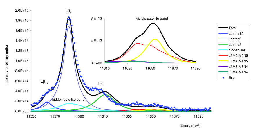
Figure 2: Gold L X-ray spectrum calculated in this work, including L$\beta_{2}$, L$\beta_{3}$, and L$\beta_{15}$ diagram lines and satellite bands, compared with the experimental data (diamonds) 11 . In the inset L$\beta_{2}$, and L$\beta_{15}$ satellite lines are shown in a different intensity scale.

3.2.3 Calculation of gold L$\beta_{2}$ satellite band using Racah’s algebra

To assess the validity of the calculation of relative satellite intensities using Racah’s algebra in the case of tungsten, we used the same procedure for the L₃M_4,5-M_4,5N₅ satellite bands of gold, where a more precise calculation allows for a comparison.

For gold, angular momenta that result from unfilled outer shells are $j_{3}=\dfrac{1}{2}$ and $j_{3}^{\prime}=\dfrac{1}{2}$. Now, in what concerns equation (19), for the L₃M₅-M₅N₅ transitions we have $J=\dfrac{1}{2},\ldots,\dfrac{9}{2}$ and $J^{\prime}=\dfrac{1}{2},\ldots,\dfrac{11}{2}$.

In order to compare the spectra generated using the two different methods, we normalized the total intensity of the L₃M₅-M₅N₅ satellite band to the same band obtained with the method described in 3.2.2.

The L₃M_4,5-M_4,5N₅ satellite bands thus obtained are presented in figure 3. The agreement obtained allows us to conclude for the validity of the tungsten L$\beta_{2}$ spectrum we generated with relative intensities obtained with Racah’s algebra.

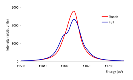
Figure 3: Calculated satellite spectrum of gold, including the L₃M_4,5-M_4,5N₅ bands, using Multi-Configuration Dirac-Fock energy values and intensities obtained with the Racah’s algebra method - Racah, and from the MCDF calculation - Full.

4 Discussion and conclusions

In this work we computed the theoretical L$\beta_{2}$ satellite band of tungsten using MCDF relativistic transition energies and a statistical model for the shape of the band.

Due to the large number of transitions involved, we were only able to estimate the position and the shape of the the L$\beta_{2}$ satellite band, using a method that employs Racah’s algebra to find relative line intensities in this band. Although the experimental values suffer from very poor statistics, our results reproduce well the main features of the measured spectrum.

In the case of gold, we used the MCDF code to compute both the transition energies and the transition probabilities of the L$\beta_{2}$, L$\beta_{3}$, L$\beta_{15}$ diagram lines as well as the L$\beta_{2}$ and L$\beta_{15}$ satellite lines, corresponding to spectator holes in the M₄ and M₅ subshells. These satellite lines are visible satellites. We also computed the energies and transition probabilities for the hidden L$\beta_{2}$ and L$\beta_{15}$ satellites. These are satellite lines, corresponding to spectator holes in the N_i ($i=1,7$), O_i ($i=1,5$), and P₁ subshells, whose energies are such that they are superimposed on the L$\beta_{2}$ diagram line.

Table 6: Energies and relative X-ray production cross sections of L$\beta_{2}$ plus L$\beta_{15}$ visible satellites for gold. Production cross sections are relative to L$\beta_{2}$ diagram line (a) and L$\beta_{2}$ diagram line plus hidden satellites (b) production cross sections, respectively.

	Energy (eV)			Relative production cross section (%)
Spectator	This	Oohashi 11		This work		Oohashi 11
hole	work	Theory	Experiment	(a)	(b)	Theory	Experiment
M5	11646.9	11648.4	11641.7$\pm$ 1.1	5.9	4.6	5.5	4.1 $\pm$ 0.4
M4	11654.0	11657.5	11658.7$\pm$ 1.1	4.4	3.5	4.2	4.1 $\pm$ 0.8

The values found in this work for the ratio of L₃M_4,5-M_4,5N_4,5 to L₃-N₅ X-ray production cross sections are presented in Table 6. For comparison with the experiment, the ratios of the L₃M_4,5-M_4,5N_4,5 to L₃-N₅ plus hidden satellites production cross sections were also computed. These ratios are compared with Oohashi et al 11 theoretical and experimental values on the same table. We note that in the latter calculation, L₃M_4,5-M_4,5N₄ satellite line production cross sections were not taken in account. Also, transition yields for satellite and diagram lines are taken by this authors as equal.

We estimate that the uncertainty in our calculation of the relative X-ray production cross sections is of the order of 20%, due mainly to the uncertainty in the L₁- and L₃-subshells ionization cross sections which are 20% and 10%, respectively.

The theoretical spectrum for gold obtained in this work agrees very well with experiment. Taking in account the uncertainties, the satellite bands relative intensities found in this work are consistent with the measured values of Oohashi et al 11 .

References

- (1) F. K. Ritchmeyer, E. G. Ramberg, Phys. Rev. 51, 925 (1937)
- (2) Juslén, M. Pessa, G. Graeffe, Phys. Rev. A 19, 196 (1979)
- (3) B. L. Doyle, S. M. Shafroth, Phys. Rev. A 19, 1433 (1979)
- (4) C. F Hague, J. -M. Mariot, G. Dufour, Phys. Lett. A 78, 328 (1980)
- (5) F. Parente, M. H. Chen, B. Crasemann, H. Mark, At. Data and Nucl. Data Tables 26, 383 (1981)
- (6) F. Parente, M. L. Carvalho, L. Salgueiro, J. Phys. B 16, 4305 (1983)
- (7) M. L. Carvalho, F. Parente, L. Salgueiro, J. Phys. B 20, 935 (1987)
- (8) L. Salgueiro, M. L. Carvalho, F. Parente, J. de Physique 48, C9-609 (1987)
- (9) J. Q. Xu, E. Rosato, Phys. Rev. A 37, 1946 (1988)
- (10) A. M. Vlaicu,T. Tochio, T. Ishizuka, D. Ohsawa, Y. Ito, T. Mukoyama, A. Nisawa, T. Shoji, S. Yoshikado, Phys. Rev. A 58, 3544 (1998)
- (11) H. Oohashi, T. Tochio, A. M. Vlaicu, Phys. Rev. A 68, 032506 (2003)
- (12) T. A. Carlson, M. Krause, Phys. Rev. 140, A1057 (1965)
- (13) M. H. Chen, B. Crasemann, H. Mark, At. Data and Nucl. Data Tables 24, 13 (1979)
- (14) M. H. Chen, B. Crasemann, K.-N. Huang, M. Aoyagi, H. Mark, At. Data and Nucl. Data Tables 19, 97 (1977)
- (15) B. K. Agarwal, X-Ray Spectroscopy, 210 (Springer-Verlag, Berlin 1979)
- (16) J. P. Desclaux, in Methods and Techniques in Computational Chemistry (STEF, Cagliary, 1993), Vol. A
- (17) P. Indelicato, Phys. Rev. Lett 77, 3323 (1996)
- (18) MCDFGME, a MultiConfiguration Dirac Fock and General Matrix Elements program, (release 2005)”, written by J. P. Desclaux and P. Indelicato (http://dirac.spectro.jussieu.fr/mcdf)
- (19) K. Dyall, I.P. Grant, C. T. Johnson, F. A. Parpia, E. P. Plummer, Comp. Phys. Commun. 55, 425 (1989)
- (20) P. O. Löwdin, Phys. Rev. 97, 1454 (1955)
- (21) P. Indelicato, Phys. Rev. A 26, 2338 (1982)
- (22) P. J. Mohr, Y.-Kim, Phys. Rev. A 45, 2727 (1992)
- (23) P. J. Mohr, Phys. Rev. A 46, 4421 (1992)
- (24) P. J. Mohr, G. Soff, Phys. Rev. Lett 70, 158 (1993)
- (25) P. Indelicato, O. Gorceix, J. P. Desclaux, J. Phys. B 20, 651 (1987)
- (26) P. Indelicato, J. P. Desclaux, Phys. Rev. A 42, 5139 (1990)
- (27) P. Indelicato, E. Lindroth, Phys. Rev. A 46, 2426 (1992)
- (28) P. Indelicato, S. Boucard, E. Lindroth, Eur. Phys. J. D 3, 29 (1998)
- (29) Campbell and Papp, At. Data and Nucl. Data Tables 77, 1 (2001)
- (30) M. O. Krause, F. Wuilleumier, C.W. Nestor, Jr., Phys. Rev. A 6, 871 (1972)
- (31) J. Pálinkas, B.Schlenk, Z. Physik A, 297, 29 (1980)
- (32) R. D. Deslattes, E. G. Kessler, Jr., P. Indelicato, L. de Billy, E. Lindroth, J. Anton, Rev. Mod. Phys. 75, 35 (2003)