Memory functions and Correlations in Additive Binary Markov Chains

Abstract

A theory of additive Markov chains with long-range memory, proposed earlier in Phys. Rev. E 68, 06117 (2003), is developed and used to describe statistical properties of long-range correlated systems. The convenient characteristics of such systems, a memory function, and its relation to the correlation properties of the systems are examined. Various methods for finding the memory function via the correlation function are proposed. The inverse problem (calculation of the correlation function by means of the prescribed memory function) is also solved. This is demonstrated for the analytically solvable model of the system with a step-wise memory function.

I Introduction

The problem of long-range correlated dynamic systems (LRCS) has been under study for a long time in many areas of contemporary physics bul ; sok ; bun ; yan ; maj ; halvin , biology vossDNA ; stan ; buld ; prov ; yul ; hao , economics stan ; mant ; zhang , literature schen ; kant ; kokol ; ebeling ; uyakm , etc. stan ; czir . One of the ways to get a correct insight into the nature of correlations in a system consists in constructing a mathematical object (for example, a correlated sequence of symbols) possessing the same statistical properties as the initial system. There exist many algorithms for generating long-range correlated sequences: the inverse Fourier transformation czir ; maks , the expansion-modification Li method li , the Voss procedure of consequent random additions voss , the correlated Levy walks shl , etc. czir . The use of the multi-step Markov chains is one of the most important among them because they offer a possibility to construct a random sequence with necessary correlated properties in the most natural way. This was demonstrated in Ref. uya , where the concept of Markov chain with the step-wise memory function was introduced. The correlation properties of some dynamical systems (coarse-grained sequences of the Eukarya’s DNA and dictionaries) can be well described by this model uya .

A sequence of symbols in the Markov chain can be thought of as the sequence of states of certain particle, which participates in a correlated Brownian motion. Thus, every $L$-word (the portion of the length $L$ in the sequence) can be considered as one of the realizations of the ensemble of correlated Brownian trajectories in the ”time” interval $L$. This point gives an opportunity to use the statistical methods for examining the correlation properties of the dynamic systems. Another important reason for the study of Markov chains is its application to the various physical objects tsal ; abe ; den , e.g., to the Ising chains of spins. The problem of thermodynamics description of the Ising chains with long-range spin interaction is still unresolved even for the 1D case. However, the association of such systems with the Markov chains can shed light on the non-extensive thermodynamics of the LRCS.

In this paper, we ascertain the relation between the memory function of the additive Markov chains and the correlation properties of the systems under consideration. We examine the simplest variant of the random sequences, dichotomic (binary) ones, although the presented theory can be applied to arbitrary additive Markov processes with finite or infinite number of states.

The paper is organized as follows. In the first Section, we introduce the general relations for the Markov chains, derive an equation connecting the correlation and memory functions of additive Markov chains, and verify the robustness of our method by numerical simulations. The second part is devoted to the study of the correlation function for the Markov chain with the step-wise memory function. In Subsec. (III.2) we reveal a band structure of the correlation function and obtain its explicit expression. Subsec. (III.3) contains the results of asymptotic study of correlation function.

II General Properties of Additive Markov Chains

II.1 Basic notions

Let us consider a homogeneous binary sequence of symbols, $a_{i}=\{0,1\}$, $i\in\textbf{{Z}}=...,-2,-1,0,1,2,...$. To determine the $N$-step Markov chain we have to introduce the conditional probability $P(a_{i}\mid a_{i-N},a_{i-N+1},\dots,a_{i-1})$ of the definite symbol $a_{i}$ (for example, $a_{i}=1$ or $a_{i}=0$ ) occurring after the $N$-word $T_{N,i}$, where $T_{N,i}$ denotes the sequence of symbols $a_{i-N},a_{i-N+1},\dots,a_{i-1}$. Thus, it is necessary to define $2^{N}$ values of the $P$-function corresponding to each possible configuration of the symbols in the $N$-word $T_{N,i}$. Since we intend to deal with the sequences possessing the memory length of the order of $10^{6}$, we need to make some simplifications. We suppose that the $P$-function has the additive form,

$$P(a_{i}=1\mid T_{N,i})=\sum\limits_{k=1}^{N}f(a_{i-k},k).$$ (1)

Here the value $f(a_{i-k},k)$ is the additive contribution of the symbol $a_{i-k}$ to the conditional probability of the symbol unity occurring at the $i$th site. Equation (1) corresponds to the additive influence of the previous symbols on the generated one. Such Markov chain is referred to as additive Markov chain, Ref. mel . The homogeneity of the Markov chain is provided by the independence of the conditional probability Eq. (1) of the index $i$. It is possible to consider Eq. (1) as the first term in expansion of conditional probability in the formal series of terms that correspond to the additive (or unary), binary, ternary, and so on functions up to $N$-ary one.

Let us rewrite Eq. (1) in an equivalent form,

$$P(a_{i}=1\mid T_{N,i})=\bar{a}+\sum\limits_{r=1}^{N}F(r)(a_{i-r}-\bar{a}).$$ (2)

Here

$$\bar{a}=\sum\limits_{r=1}^{N}f(0,r)/[1-\sum\limits_{r=1}^{N}(f(1,r)-f(0,r))]$$

is the average number of unities in the sequence, Ref. mel , and

$$F(r)=f(1,r)-f(0,r).$$

We refer to $F(r)$ as the memory function (MF). It describes the strength of impact of previous symbol $a_{i-r}$ upon a generated one, $a_{i}$. Evidently, this function has to satisfy condition $0\leqslant P(a_{i}=1\mid T_{N,i})\leqslant 1$. To the best of our knowledge, the concept of the memory function for multi-step Markov chains was introduced in papers uyakm ; uya where it is shown that it is convenient to use it in describing the correlated properties of complex dynamical systems with long-range correlations.

The function $P(a_{i}=1\mid T_{N,i})$ contains complete information about correlation properties of the Markov chain. In general, the correlation function and other moments are employed as the input characteristics for the description of the correlated random systems. Yet, the correlation function takes account of not only the direct interconnection of the elements $a_{i}$ and $a_{i+r}$, but also their indirect interaction via other elements. Our approach operates with the “origin” characteristics of the system, specifically with the memory function.

The positive values of the MF result in persistent diffusion where previous displacements of the Brownian particle in some direction provoke its consequent displacement in the same direction. The negative values of the MF correspond to the antipersistent diffusion where the changes in the direction of motion are more probable. In terms of the Ising long-range particles interaction model, which could be naturally associated with the Markov chains, the positive values of the MF correspond to the attraction of particles and negative ones conform to the repulsion.

We consider the distribution $W_{L}(k)$ of the words of definite length $L$ by the number $k$ of unities in them, $k_{i}(L)=\sum\limits_{l=1}^{L}a_{i+l}$, and the variance $D(L)$ of $k_{i}(L)$,

$$D(L)=\overline{(k-\bar{k})^{2}},$$ (3)

where the definition of average value of $g(k)$ is $\overline{g(k)}=\sum\limits_{k=0}^{L}g(k)W_{L}(k)$.

Another statistical characteristics of random sequences is the correlation function,

$$K(r)=\overline{a_{i}a_{i+r}}-\bar{a}^{2}.$$ (4)

By definition, the correlation function is even, $K(-r)=K(r)$, and $K(0)=\bar{a}(1-\bar{a})$ is the variance of the random variable $a_{i}$. The correlation function is connected with the above mentioned variance by the equation

$$K(r)=\frac{1}{2}(D(r-1)-2D(r)+D(r+1)),$$ (5)

or

$$K(r)=\frac{1}{2}\frac{\textrm{d}^{2}D(r)}{\textrm{d}r^{2}}$$ (6)

in the continuous limit.

II.2 Derivation of main equation

In this subsection we obtain a very important relation connacting the memory and correlation functions of the additive Markov chain. Let us introduce the function $\phi(r)=p(a_{i}=1\mid a_{i-r}=1)$, which is the probability of symbol $a_{i}=1$ occurring under condition that previous symbol $a_{i-r}$ is also equal to unity. This function is obviously connected to the correlation function $K(r)$, see Eq. (4) since the quantity $\overline{a_{i}a_{i-r}}$ is the probability of simultaneous equality to unity of both symbols, $a_{i}$ and $a_{i-r}$. It can be expressed in terms of the conditional probability $\phi(r)$,

$$\overline{a_{i}a_{i-r}}=\bar{a}\phi(r).$$ (7)

Substituting Eq. (2) into Eq. (4) we get:

$$K(r)=\bar{a}\phi(r)-\bar{a}^{2}.$$ (8)

For the $N$-step Markov chain, the probability of the symbol $a_{i}=1$ occurring depends only on the previous $N$-word. Therefore, to obtain the value of $\phi(r)$ one needs to average the conditional probability $P$ Eq. (2) over all realizations of the $N$-words with the condition $a_{i-r}=1$,

$$\phi(r)=p(a_{i}=1\mid a_{i-r}=1)$$ (9)

$$=\sum\limits_{T_{N,i}}P(a_{i}=1\mid T_{N,i})p(T_{N,i}\mid a_{i-r}=1).$$

If the value of $r$ is less or equal to $N$, then $a_{i-r}$ in Eq. (9) is one of the symbols $a_{i-1},a_{i-2},\dots,a_{i-N}$ in the word $T_{N,i}$. In this case, the sum in Eq. (9) allows not all $N$-words, but only the words that contain the symbol unity at the $(i-r)$th position. If $r>N$, the memory function $F(r)$ equals zero in this region and, therefore, the sum in Eq. (9) contains all terms corresponding to all different $N$-words.

Substituting Eq. (2) into Eq. (9), we obtain:

$$\phi(r)=\bar{a}\sum\limits_{T_{N,i}}P(T_{N,i}\mid a_{i-r}=1)$$ (10)

$$+\sum\limits_{r^{\prime}=1}^{N}F(r^{\prime})\sum\limits_{T_{N,i}}(a_{i-r^{\prime}}-\bar{a})P(T_{N,i}\mid a_{i-r}=1).$$

According to the normalization condition, the first sum in Eq. (10) is equal to unity. Consider the sum

$$\sum\limits_{T_{N,i}}a_{i-r^{\prime}}P(T_{N,i}\mid a_{i-r}=1)$$ (11)

in the second term in RHS of Eq. (10). The symbol $a_{i-r^{\prime}}$ is contained within the word $T_{N,i}$. Therefore, Eq. (11) represents the average value of $a_{i-r^{\prime}}$ under condition $a_{i-r}=1$. In other words, it equals the probability $\phi(r-r^{\prime})$ of $a_{i-r^{\prime}}=1$ occurring under the condition $a_{i-r}=1$:

$$\sum\limits_{w}a_{i-r^{\prime}}P(T_{N,i}\mid a_{i-r}=1)=\phi(r-r^{\prime}).$$ (12)

Substituting this equation into Eq. (10) we obtain:

$$\phi(r)=\bar{a}+\sum\limits_{r^{\prime}=1}^{N}F(r^{\prime})(\phi(r-r^{\prime})-\bar{a}).$$ (13)

Taking into account Eq. (8), we arrive at the relation between the memory function and the correlation function:

$$K(r)=\sum\limits_{r^{\prime}=1}^{N}F(r^{\prime})K(r-r^{\prime}),\qquad r\geqslant 1.$$ (14)

This equation was first derived by the variation method in Ref. mel .

Another equation resulting from Eq. (14) by double summation over index $r$ establishes a relationship between the memory function $F(r)$ and the variance $D(L)$,

$$M(r,0)=\sum\limits_{r^{\prime}=1}^{N}F(r^{\prime})M(r,r^{\prime}),$$ (15)

$$M(r,r^{\prime})=D(r-r^{\prime})-(D(-r^{\prime})+r[D(-r^{\prime}+1)-D(-r^{\prime})]).$$

Equation (5) and parity of the function $D(r)$ are used here.

The last equation shows convenience of using the variance $D(L)$ instead of the correlation function $K(r)$. The function $K(r)$, being a second derivative of $D(r)$ in continuous approximation, is less robust in computer simulations. It is the main reason why we prefer to use Eq. (15) for the long-range memory sequences. This is our tool for finding the memory function $F(r)$ of a sequence using the variance $D(L)$.

II.3 Numerical reconstruction of the memory function

Let us verify the robustness of our method by numerical simulations. We consider a model memory function,

$$F(r)=0.1\cases{1-r/10,\;\qquad\;\;\ 1\leqslant r<10,\cr 0,\;\;\;\;\;\;\;\;\;\;\ \qquad\qquad r\geqslant 10.}$$ (16)

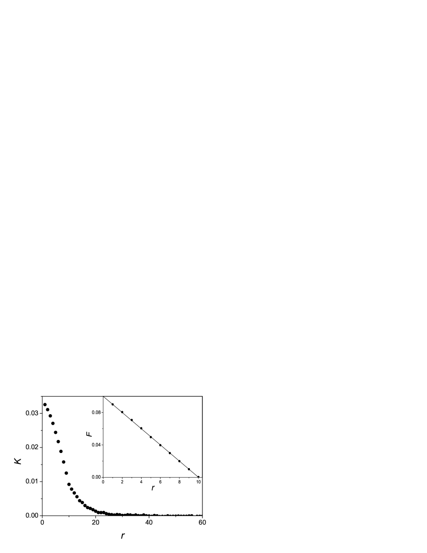
Figure 1: Calculated correlation function $K(r)$ of the Markov chain constructed with the model memory function $F(r)$, Eq. (16), shown by the solid line in the inset. Dots in the inset correspond to the memory function reconstructed by solving Eq. (14) with correlation function $K(r)$ presented in the main panel.

shown in the inset in Fig. 1 by solid line. Using Eq. (2), we construct a random unbiased $\bar{a}=1/2$, Markov chain. Then, with the help of the constructed binary sequence of the length $3\times 10^{6}$, we calculate numerically the correlation function $K(r)$ by solving the set of $N$ linear equations (14). The result of these calculations is given in Fig. 1. One can see that the correlation function $K(r)$ mimics roughly the memory function $F(r)$ over the region $1\leqslant r\leqslant 10$. In the region $r>10$, the memory function is equal to zero but the correlation function does not vanish ref . Then, using the obtained correlation function $K(r)$, we solve numerically Eq. (14). The result is shown in the inset in Fig. 1 by dots. One can see an excellent agreement of initial, Eq. (16), and reconstructed memory functions $F(r)$.

The ability of constructing a binary sequence with an arbitrary prescribed correlation function by means of Eq. (14) is the very nontrivial result of this paper.

Yet another approach to numerical finding the memory function is an iteration procedure. For its realization let us rewrite Eq. (14) in the form,

$$F(r)=\frac{K(r)}{K(0)}-\!\!\!\sum\limits_{r^{\prime}=1,\ r^{\prime}\neq r}^{N}\!\!\!\frac{K(r-r^{\prime})}{K(0)}F(r^{\prime}).$$ (17)

Using Eq. (17) with starting iteration $F_{0}(r)=0$, we obtain the formula,

$$F_{n+1}(r)=\frac{K(r)}{K(0)}-\!\!\!\sum\limits_{r^{\prime}=1,\ r^{\prime}\neq r}^{N}\!\!\!\frac{K(r-r^{\prime})}{K(0)}F_{n}(r^{\prime}),\,n\geqslant 0.$$ (18)

Thus, the memory function can be presented as the series,

$$F(r)=\frac{K(r)}{K(0)}-\sum\limits_{r^{\prime}\neq r}\frac{K(r-r^{\prime})K(r^{\prime})}{K^{2}(0)}+\sum\limits_{r^{\prime}\neq r}\sum\limits_{r^{\prime\prime}\neq r^{\prime}}\frac{K(r-r^{\prime})K(r^{\prime}-r^{\prime\prime})K(r^{\prime\prime})}{K^{3}(0)}+\dots$$ (19)

Note, that the Markov chain with the definite correlation function $K(r)$ exists if the series (19) is convergent and the obtained function implies the probability Eq. (2) satisfying the requirement $0\leqslant P(a_{i}=1\mid T_{N,i})\leqslant 1$ for arbitrary word $T_{N,i}$. If $\bar{a}=1/2$ we obtain the restriction, $\sum|F(r)|\leqslant 1$. The sufficient, but not necessary, requirement is $\sum\limits_{r=1}^{N-1}|K(r)|\leqslant 1/12-|K(N)|/3$.

III CORRELATION FUNCTION of the chain with the step-wise memory function

In the previous section, we obtained the relationship (14) between two characteristics of the Markov chain, the memory and correlation functions, and used this equation to solve the problem of finding the memory function via the known correlation function. Here we present the solution of the inverse problem. We suppose the memory function to be known and find the correlation function of the corespondent Markov chain. To simplify our consideration, we examine the step-wise memory function,

$$F(r)=\cases{\alpha,\quad r\leqslant N,\cr 0,\quad r>N.}$$ (20)

The restriction imposed on the parameter $\alpha$ can be obtained from Eq. (2): $|\alpha|<1/N$. Note that each of the symbols unity in the preceding N-word promotes the emergence of new symbol unity if $0<\alpha<1/N$. This corresponds to the persistent diffusion. The region of parameter $\alpha$, determined by inequality $-1/N<\alpha<0$, corresponds to the anti-persistent diffusion. If $\alpha=0$, one arrives at the case of the non-correlated Brownian motion.

III.1 Main equation for the correlation function

Substituting Eq. (20) into Eq. (14) we obtain the relation,

$$K(r)=\alpha\sum\limits_{r^{\prime}=1}^{N}K(r-r^{\prime}),\quad r\geqslant 1.$$ (21)

Here, the correlation function is assumed to be even, $K(-r)=K(r)$. Equation (21) is the linear recurrence of the order of $N$ for $r\geqslant N+1$, so we stand in need of $N$ initial conditions. For the unbiased sequence, $\bar{a}=1/2$, we have $K(0)=1/4$. The solution of Eqs. (21) written for $r=1,\dots,N$ yields the constant value of the correlation function, $K(r)=K_{0}$ at $r=1,\dots,N-1$,

$$K_{0}=\frac{\alpha}{4(1-\alpha(N-1))}.$$ (22)

Subtracting Eq. (21) from the same equation written for $r+1$, we derive another, more convenient, form of the recurrence:

$$K(r+1)-(1+\alpha)\leavevmode\nobreak\ K(r)+\alpha\leavevmode\nobreak\ K(r-N)=0.$$ (23)

This equation is of the order of $N+1$, thus we need an additional initial condition. It can be derived from Eq. (21): $K(N)=K_{0}$. Note that the possibility to rewrite Eq. (21) in the form of Eq. (23) is the result of the simple structure of the memory function. We solve the obtained recurrent equations by the most natural method, by means of step-by-step finding the sequent values of the correlation function. Such an approach is very suitable for the analysis of correlation function at $r\gtrsim N$.

III.2 Correlation function at $r\gtrsim N$

III.2.1 Band structure of the correlation function

Equation (21) allows one to find numerically the unknown correlation function $K(r)$. The result of this step-by-step calculation is presented in Fig. 2 by solid line.

Figure 2: Correlation function $K(r)$ (solid line) obtained by two different methods: the numerical simulation of Eq. (14) and exact solution Eq. (41). The dotted line is for the contribution to $K(r)$ of the first root of Eq. (32). The dashed line refers to the correlation function obtained in uyakm . The vertical lines indicate the limits of the bands numbered by $s$.

One can easily see the discontinuity of $K(r)$ at the point $L=N=100$, the breakpoint of the curve is observed at $L=2N$. Such behavior of the correlation function is the result of using the memory function of the step-wise form. To clarify this fact it is convenient to change the variable $r$ by the band number $s$ and the intra-band number $\rho$:

$$K(r)=K_{s}(\rho),\qquad r=sN+\rho+1,\quad\rho=0,1,\ldots,N-1,\;s=0,1,\ldots.$$ (24)

Within $s$th band, Eq. (23) is the recurrence of the second order with the term $\alpha\,K_{s-1}(\rho)$ that is determined at the previous step, while finding the correlation function for the $(s-1)$th band.

III.2.2 General expression for the correlation function

In the zeroth band ($s=0,\leavevmode\nobreak\ 1\leqslant r\leqslant N$), as it was shown above, the correlation function is constant,

$$K_{0}(\rho)=K_{0}.$$ (25)

For the first band ($s=1,\leavevmode\nobreak\ N+1\leqslant r\leqslant 2N$), taking into account that $K(r-N-1)=K_{0}(\rho)$, we have

$$K_{1}(\rho)=K_{0}\,(1-(1-\alpha N)(1+\alpha)^{\rho}).$$ (26)

The correlation function decreases quasi-continuously within the first band. However, as it was mentioned above, there exists a discontinuity in the $K(r)$ dependence at $r=N$. This discontinuity disappears in the limiting case of the strong persistence, $\alpha\rightarrow 1/N$.

Substituting the obtained formula (26) in Eq. (23), we find the solution $K_{2}(\rho)$ for the second band ($s=2,\leavevmode\nobreak\ 2N+1\leqslant r\leqslant 3N$),

$$K_{2}(\rho)=K_{0}\,(1-(1-\alpha N)((1+\alpha)^{\rho+N}-\rho\,\alpha(1+\alpha)^{\rho-1}).$$ (27)

The correlation function $K(r)$ is continuous at the interface between the first and second bands, $K_{1}(N)=K_{2}(0)$. However, its first derivative of $K(r)$ is discontinuous here (see Fig. 2). Using the induction method, one can easily derive the formula for $K_{s}(\rho)$ in the $s$th band ($sN+1\leqslant r\leqslant(s+1)N$):

$$K_{s}(\rho)=K_{0}\,\left(1-(1-\alpha N)\sum\limits_{i=1}^{s}(-\alpha)^{i-1}(1+\alpha)^{(s-i)N+\rho-i+1}\text{C}_{(s-i)N+\rho}^{i-1}\right),$$ (28)

$$\quad C_{n}^{k}=\frac{\Gamma(n+1)}{\Gamma(k+1)\Gamma(n-k+1)}.$$

It follows from Eq. (28), that the first $(s-2)$ derivatives of the correlation function $K(r)$ are continuous at the border between the $(s-1)$th and $s$th bands, but the derivative of the $(s-1)$th order changes discontinuously. Under the condition $\alpha N\ll 1$, Eq. (28) takes a simpler form,

$$K_{s}(\rho)=K_{0}\alpha^{s}\text{C}_{s+N-1-\rho}^{s}.$$ (29)

It is seen that the correlation function decreases proportionally to $\alpha^{s}$ with an increase of the band number $s$.

It is not easy to analyze the asymptotical behavior of the function $K(r)$ at large $s$ because the number of summands in Eq. (28) increases being proportional to $s$. It is the reason to propose another approach for the asymptotical study of the correlation function $K(r)$ at $s\gg 1$.

III.3 Asymptotical study of the correlation function

III.3.1 Derivation of the characteristic equation

The general solution of linear recursion equations (21) can be represented as the linear combination of $N$ different exponential functions,

$$K(r)=\sum\limits_{i=1}^{N}a_{i}\xi_{i}^{r}.$$ (30)

To find the values of $\xi_{i}$, we substitute the fundamental solution,

$$K(r)=\xi^{r},$$ (31)

into Eq. (21) and obtain the characteristic polynomial equation of the order of $N$. Constant multipliers $a_{i}$ are to be determined by initial conditions.

It is more convenient to use Eq. (23) instead of Eq. (21), that implies the characteristic equation of the order of $N+1$,

$$\xi^{N+1}-(1+\alpha)\xi^{N}+\alpha=0.$$ (32)

The extra root of this equation, $\xi=1$, appears as a consequence of passing on to the equation of order of $N+1$ from that of the order of $N$ . The corresponding coefficient, $a_{i}$, in Eq. (30) is equal to zero because the correlation function should decrease at $r\rightarrow\infty$.

Our study shows that Eq. (32) has one real positive root less than unity in the case of odd $N$. In the case of even $N$, there are two real roots, one positive and one negative. The remaining roots are complex. All absolute values of roots are less than unity, that is in agreement with the finiteness of memory function $F(r)$. In the case of large $N$, the absolute magnitudes of all roots are close to unity for nearly all values of $\alpha$ satisfying the inequality,

$$\frac{1}{N}\ln{\frac{1}{\alpha}}\ll 1.$$ (33)

Distribution of the roots in the complex plane $\xi$ is shown in Fig. 3.

Figure 3: The dots are the roots of the characteristic equation (32) for $N=100$ and $\alpha=0.008$. The solid line is the circle $|\xi|=1$.

In the simplest case, $N=2$, Eq. (32) has two real roots,

$$\xi_{1,\leavevmode\nobreak\ 2}=\frac{\alpha}{2}\pm\sqrt{\frac{\alpha^{2}}{4}+\alpha}.$$ (34)

Taking into account the initial conditions, we find the solution of Eq. (21) in the form,

$$K(r)=\frac{\alpha}{4(1-\alpha)\sqrt{\alpha^{2}+4\alpha}}(\xi_{1}^{r-1}(1-\xi_{2})-\xi_{2}^{r-1}(1-\xi_{1})).$$ (35)

This expression can be simplified at small and large values of parameter $\alpha$. For $\alpha\ll 1$, one obtains

$$K(r)=\frac{1}{4}\alpha^{[r/2]+1}$$ (36)

with square brackets standing for the integer part. The correlation function in the sequent odd and even points are equal to each other. In accordance with Eq. (29), $K(r)$ decreases at $r\rightarrow\infty$ being proportional to $\alpha^{s}$. In the opposite limiting case of the strong persistency, $\alpha\rightarrow 1/2$, we have two different roots,

$$\xi_{1}=1-\frac{4}{3}\leavevmode\nobreak\ \phi,\qquad\xi_{2}=-\frac{1}{2}+\frac{1}{3}\leavevmode\nobreak\ \phi,$$ (37)

with $\phi=1/2-\alpha$. The coefficient corresponding to the second root is much less than that corresponding to the first one. Besides, the second term in Eq. (35) decreases more rapidly. Therefore, the approximate solution in this case is

$$K(r)=\frac{1}{4}\exp{-4\phi(r-1)/3}.$$ (38)

III.3.2 Correlation function at small $\alpha$

Let us return to the case of arbitrary value of $N$. If $\alpha$ is very small, i.e. at

$$\frac{1}{N}\ln{\frac{1}{\alpha}}\gg 1,$$ (39)

Eq. (32) has $N$ roots with small absolute magnitudes:

$$\xi_{k}=\alpha^{1/N}(\cos(2\pi\frac{k}{N})+i\sin(2\pi\frac{k}{N})),\qquad k=0,\ldots,N-1.$$ (40)

The correlation function, being a linear combination of the power functions with these roots as their exponents, decreases proportionally to $\alpha^{s}$, which agrees with Eq. (29).

The coefficients $a_{i}$ in the linear combination Eq. (30) can be found in a general case, without any restrictions imposed on the value of $\alpha$. The solution of Eq. (21) written for $1\leqslant r\leqslant N-1$ along with $K(0)=1/4$ can be expressed with the help of the Vandermond determinants:

$$K(r)=K_{0}(\alpha N-1)\sum\limits_{k=1}^{N}\frac{\xi_{k}^{r-1}}{\prod\limits_{j=1,j\neq k}^{N+1}(\xi_{k}-\xi_{j})},$$ (41)

with $\xi_{N+1}=1$.

III.3.3 Correlation function at not too small $\alpha$

In the case (33) of not too small $\alpha$, the absolute magnitudes of all roots are close to unity. It is convenient to rewrite Eq. (32), introducing two new real variables $\gamma$ and $\varphi$ instead of complex $x$ according to

$$x=(1-\frac{1}{\gamma N})e^{i\varphi}.$$ (42)

Equation (32) takes the form,

$$\alpha(e^{\frac{1}{\gamma}-iN\varphi}-1)=(1-\frac{1}{\gamma N})e^{i\varphi}-1.$$ (43)

For the real root, Eq. (32) yields,

$$\alpha N\gamma(e^{1/\gamma}-1)=1.$$ (44)

This expression along with Eq. (31) determines the asymptotical behavior of correlation function. It was first obtained in Ref. uyakm . The qualitative approach of this paper did not allow one to take into account the contribution of other roots as it is done in the present paper.

Equation (43) yields all remaining complex roots with the values of $\varphi$, which are quite uniformly distributed over the circle $[0,2\pi]$ and

$$\frac{1}{\gamma}\sim\ln{\frac{1}{\alpha}}.$$ (45)

The roots of Eq. (32) located in the vicinity of point $\xi=1$ are shown in Fig. 4. The single real root is much closer to the line $\texttt{Re}\,\,\xi=1$ than the other ones. Besides, the coefficients $a_{i}$ in Eq. (41) (see also Eq. (30)) for all terms containing the complex exponents are much less than those for the term with the real exponent. Therefore, the behavior of correlation function $K(r)$ is determined generally by the term with the real exponent.

Figure 4: The roots of characteristic polynomial equation close to the point $\xi=1$ for $N=4000$, $\alpha=2\cdot 10^{-4}$. The solid line is $\texttt{Re}\,\,\xi=1$.

The exact correlation function $K(r)$ resulting from the numerical simulation of Eq. (41) and its approximation determined by the contribution of the real root alone are shown in Fig. 2. These curves are compared with that obtained in Ref. uyakm by a qualitative method.

The obtained correlation function can be used to calculate one of the most important characteristics of the random binary sequences, the variance of number of unities in the $L$-word. The results of the numerical simulations are shown in Fig. 5. One can see a good agreement of curves plotted using both of these methods.

Figure 5: Variance $D(L)$ for the Markov chain with $N=100$, $\alpha=0.008$ obtained by means of exact Eqs. (41), (5) (solid line) and using only one root of Eq. (32) (dashed line). The thin solid line describes the non-correlated Brownian diffusion, $D(L)=L/4$.

III.3.4 Conclusion

Thus, we have demonstrated the efficiency of describing the symbolic sequences with long-range correlations in terms of the many-step Markov chains with the additive memory function. Actually, the memory function appears to be a suitable informative ”visiting card” of any symbolic stochastic process. Various methods for finding the memory function via the correlation function of the system are proposed. Our preliminary consideration shows the possibility to generalize our concept of the Markov chains on larger class of random processes where the random variable can take on arbitrary, finite or infinite number of values.

The suggested approach can be used for the analysis of different correlated systems in various fields of science. For example, the application of the Markov sequences to the theory of spin chains with long-range interaction makes it possible to estimate some thermodynamic characteristics of these non-extensive systems.

References

- (1) U. Balucani, M. H. Lee, V. Tognetti, Phys. Rep. 373, 409 (2003).
- (2) I. M. Sokolov, Phys. Rev. Lett. 90, 080601 (2003).
- (3) A. Bunde, S. Havlin, E. Koscienly-Bunde, H.-J. Schellenhuber, Physica A 302, 255 (2001).
- (4) H. N. Yang, Y.-P. Zhao, A. Chan, T.-M. Lu, and G. C. Wang, Phys. Rev. B56, 4224 (1997).
- (5) S. N. Majumdar, A. J. Bray, S. J. Cornell, and C. Sire, Phys. Rev. Lett. 77, 3704 (1996).
- (6) S. Halvin, R. Selinger, M. Schwartz, H. E. Stanley, and A. Bunde, Phys. Rev. Lett. 61, 1438 (1988).
- (7) R. F. Voss, Phys. Rev. Lett. 68, 3805 (1992).
- (8) H. E. Stanley et. al., Physica A 224,302 (1996).
- (9) S. V. Buldyrev, A. L. Goldberger, S. Havlin, R. N. Mantegna, M. E. Matsa, C.-K. Peng, M. Simons, H. E. Stanley, Phys. Rev. E51, 5084 (1995).
- (10) A. Provata and Y. Almirantis, Physica A 247, 482 (1997).
- (11) R. M. Yulmetyev, N. Emelyanova, P. Hänggi, and F. Gafarov, A. Prohorov, Phycica A 316, 671 (2002).
- (12) B. Hao, J. Qi, Mod. Phys. Lett., 17, 1 (2003).
- (13) R. N. Mantegna, H. E. Stanley, Nature (London) 376, 46 (1995).
- (14) Y. C. Zhang, Europhys. News, 29, 51 (1998).
- (15) A. Schenkel, J. Zhang, and Y. C. Zhang, Fractals 1, 47 (1993).
- (16) I. Kanter and D. A. Kessler, Phys. Rev. Lett. 74, 4559 (1995).
- (17) P. Kokol, V. Podgorelec, Complexity International, 7, 1 (2000).
- (18) W. Ebeling, A. Neiman, T. Poschel, arXiv:cond-mat/0204076.
- (19) O. V. Usatenko, V. A. Yampol’skii, K. E. Kechedzhy and S. S. Mel’nyk, Phys. Rev. E 68, 06117 (2003).
- (20) A. Czirok, R. N. Mantegna, S. Havlin, and H. E. Stanley, Phys. Rev. E52, 446 (1995).
- (21) H. A. Makse, S. Havlin, M. Schwartz, and H. E. Stanley, Phys. Rev. E53, 5445 (1995).
- (22) W. Li, Europhys. Let. 10, 395 (1989).
- (23) R. F. Voss, in: Fundamental Algorithms in Computer Graphics, ed. R. A. Earnshaw (Springer, Berlin, 1985) p. 805.
- (24) M. F. Shlesinger, G. M. Zaslavsky, and J. Klafter, Nature (London) 363, 31 (1993).
- (25) O. V. Usatenko and V. A. Yampol’skii, Phys. Rev. Lett. 90, 110601 (2003).
- (26) C. Tsalis, J. Stat. Phis. 52, 479 (1988).
- (27) Nonextensive Statistical Mechanics and Its Applications, eds. S. Abe and Yu. Okamoto (Springer, Berlin, 2001).
- (28) S. Denisov, Phys. Lett. A, 235, 447 (1997).
- (29) S. S. Melnyk, O. V. Usatenko, and V. A. Yampol’skii, Physica A, 361, 405 (2006).
- (30) The existence of the ”additional tail” in the correlation function is in agreement with Ref. uyakm and corresponds to the well known fact that the correlation length is always larger then the region of memory function action.