IN PLASMA PHYSICS.

PART II: VLASOV-LIKE SYSTEMS.

IMPORTANT REDUCTIONS

Antonina N. Fedorova, Michael G. Zeitlin IPME RAS, St. Petersburg, V.O. Bolshoj pr., 61, 199178, Russia

e-mail: zeitlin@math.ipme.ru

e-mail: anton@math.ipme.ru

http://www.ipme.ru/zeitlin.html

http://www.ipme.nw.ru/zeitlin.html LOCALIZATION AND FUSION MODELING IN PLASMA PHYSICS. PART II: VLASOV-LIKE SYSTEMS. IMPORTANT REDUCTIONS Antonina  N. Fedorova and Michael  G. Zeitlin IPME RAS, Russian Academy of Sciences, V.O. Bolshoj pr., 61, 199178, St. Petersburg, Russia http://www.ipme.ru/zeitlin.html; http://www.ipme.nw.ru/zeitlin.html Abstract The methods developed in the previous Part I are applied to a few important reductions of BBGKY hierarchy, namely, various examples of Vlasov-like systems. It is well known that they are important both for fusion modeling and for particular physical problems related to plasma/beam physics. As in part I we concentrate mostly on phenomena of localization and pattern formation. Abstract The methods developed in the previous Part I are applied to a few important reductions of BBGKY hierarchy, namely, various examples of Vlasov-like systems. It is well known that they are important both for fusion modeling and for particular physical problems related to plasma/beam physics. As in part I we concentrate mostly on phenomena of localization and pattern formation. Two lectures presented at the Sixth Symposium on Current Trends in International Fusion Research, Washington D.C., March, 2005,

edited by Emilio Panarella, NRC Reasearch Press, National Reasearch Council of Canada, Ottawa, Canada, 2006.

1 INTRODUCTION: VLASOV-POISSON SYSTEM

1.1 Description

In this part we present the applications of our approach based on variational multiresolution technique [1]-[6], considered in Part I [7], to the systems with collective type behaviour described by some forms of Vlasov-Poisson/Maxwell equations, some important reduction of general BBGKY hierarchy [8]. Such approach may be useful in all models in which it is possible and reasonable to reduce all complicated problems related to statistical distributions to the problems described by the systems of nonlinear ordinary/partial differential/integral equations with or without some (functional) constraints. In periodic accelerators and transport systems at the high beam currents and charge densities the effects of the intense self-fields, which are produced by the beam space charge and currents, determinine (possible) equilibrium states, stability and transport properties according to underlying nonlinear dynamics. The dynamics of such space-charge dominated high brightness beam systems can provide the understanding of the instability phenomena such as emittance growth, mismatch, halo formation related to the complicated behaviour of underlying hidden nonlinear modes outside of perturbative tori-like KAM regions [8]. Our analysis based on the variational-wavelet approach allows to consider polynomial and rational type of nonlinearities. In some sense in this particular case this approach is direct generalization of traditional nonlinear $\delta F$ approach [8] in which weighted Klimontovich representation

$$\delta f_{j}=a_{j}\sum^{N_{j}}_{i=1}w_{ji}\delta(x-x_{ji})\delta(p-p_{ji})$$ (1)

or self-similar decompostion like

$$\delta n_{j}=b_{j}\sum^{N_{j}}_{i=1}w_{ji}s(x-x_{ji}),$$ (2)

where $s(x-x_{ji})$ is a shape function of distributing particles on the grids in configuration space, are replaced by powerful technique from local nonlinear harmonic analysis, based on underlying symmetries of functional space such as affine or more general. The solution has the multiscale/multiresolution decomposition via nonlinear high-localized eigenmodes, which corresponds to the full multiresolution expansion in all underlying time/phase space scales. Starting from Vlasov-Poisson equations, we consider the approach based on multiscale variational-wavelet formulation. We give the explicit representation for all dynamical variables in the base of compactly supported wavelets or nonlinear eigenmodes. Our solutions are parametrized by solutions of a number of reduced algebraical problems, one from which is nonlinear with the same degree of nonlinearity as initial problem and the others are the linear problems which correspond to the particular method of calculations inside concrete wavelet scheme. Because our approach started from variational formulation we can control evolution of instability on the pure algebraical level of reduced algebraical system of equations. This helps to control stability/unstability scenario of evolution in parameter space on pure algebraical level. In all these models numerical modeling demonstrates the appearance of coherent high-localized structures and as a result the stable patterns formation or unstable chaotic behaviour. Analysis based on the non-linear Vlasov equations leads to more clear understanding of collective effects and nonlinear beam dynamics of high intensity beam propagation in periodic-focusing and uniform-focusing transport systems. We consider the following form of equations

$$\Big{\{}\frac{\partial}{\partial s}+p_{x}\frac{\partial}{\partial x}+p_{y}\frac{\partial}{\partial y}-\Big{[}k_{x}(s)x+\frac{\partial\psi}{\partial x}\Big{]}\frac{\partial}{\partial p_{x}}-$$

$$\Big{[}k_{y}(s)y+\frac{\partial\psi}{\partial y}\Big{]}\frac{\partial}{\partial p_{y}}\Big{\}}f_{b}(x,y,p_{x},p_{y},s)=0,$$ (3)

$$\Big{(}\frac{\partial^{2}}{\partial x^{2}}+\frac{\partial^{2}}{\partial y^{2}}\Big{)}\psi=-\frac{2\pi K_{b}}{N_{b}}\int\mathrm{d}p_{x}\mathrm{d}p_{y}f_{b},$$

$$\int\mathrm{d}x\mathrm{d}y\mathrm{d}p_{x}\mathrm{d}p_{y}f_{b}=N_{b}.$$

The corresponding Hamiltonian for transverse single-particle motion is given by

$$H(x,y,p_{x},p_{y},s)=\frac{1}{2}(p_{x}^{2}+p_{y}^{2})+\frac{1}{2}[k_{x}(s)x^{2}$$ (4)

$$+k_{y}(s)y^{2}]+H_{1}(x,y,p_{x},p_{y},s)+\psi(x,y,s),$$

where $H_{1}$ is nonlinear (polynomial/rational) part of the full Hamiltonian and corresponding characteristic equations are:

$$\frac{\mathrm{d}^{2}x}{\mathrm{d}s^{2}}+k_{x}(s)x+\frac{\partial}{\partial x}\psi(x,y,s) = 0,$$ (5)

$$\frac{\mathrm{d}^{2}y}{\mathrm{d}s^{2}}+k_{y}(s)y+\frac{\partial}{\partial y}\psi(x,y,s) = 0.$$

1.2 Multiscale Representation

We obtain our multiscale/multiresolution representations for solutions of these equations via variational-wavelet approach. We decompose the solutions as

$$f_{b}(s,x,y,p_{x},p_{y})=\sum^{\infty}_{i=i_{c}}\oplus\delta^{i}f(s,x,y,p_{x},p_{y}),$$ (6)

$$\psi(s,x,y)=\sum^{\infty}_{j=j_{c}}\oplus\delta^{j}\psi(s,x,y),$$

$$x(s)=\sum^{\infty}_{k=k_{c}}\oplus\delta^{k}x(s),$$

$$y(s)=\sum^{\infty}_{\ell=\ell_{c}}\oplus\delta^{\ell}y(s),$$

where set

$$(i_{c},j_{c},k_{c},\ell_{c})$$ (7)

corresponds to the coarsest level of resolution $c$ in the full multiresolution decomposition [9]

$$V_{c}\subset V_{c+1}\subset V_{c+2}\subset\dots$$ (8)

Introducing detail space $W_{j}$ as the orthonormal complement of $V_{j}$ with respect to

$$V_{j+1}:V_{j+1}=V_{j}\bigoplus W_{j},$$ (9)

we have for

$$f,\psi,x,y\subset L^{2}({\bf R})$$ (10)

$$L^{2}({\bf R})=\overline{V_{c}\displaystyle\bigoplus^{\infty}_{j=c}W_{j}}.$$ (11)

In some sense it is some generalization of the old $\delta F$ approach [8]. Let $L$ be an arbitrary (non) linear differential/integral operator with matrix dimension $d$, which acts on some set of functions

$$\Psi\equiv\Psi(s,x)=\Big{(}\Psi^{1}(s,x),\dots,\Psi^{d}(s,x)\Big{)},\ s,x\in\Omega\subset{\bf R}^{n+1}$$ (12)

from $L^{2}(\Omega)$:

$$L\Psi\equiv L(R(s,x),s,x)\Psi(s,x)=0,$$ (13)

where $x$ are the generalized space coordinates or phase space coordinates, and $s$ is ”time” coordinate. After some anzatzes the main reduced problem may be formulated as the system of ordinary differential equations

$$Q_{i}(f)\frac{\mathrm{d}f_{i}}{\mathrm{d}s}=P_{i}(f,s),\quad f=(f_{1},...,f_{n}),$$ (14)

$$i=1,\dots,n,\quad\max_{i}deg\ P_{i}=p,\quad\max_{i}deg\ Q_{i}=q$$

or a set of such systems corresponding to each independent coordinate in phase space. They have the fixed initial (or boundary) conditions $f_{i}(0)$, where $P_{i},Q_{i}$ are not more than polynomial functions of dynamical variables $f_{j}$ and have arbitrary dependence on time. As result we have the following reduced algebraic system of equations on the set of unknown coefficients $\lambda_{i}^{k}$ of localized eigenmode expansion:

$$L(Q_{ij},\lambda,\alpha_{I})=M(P_{ij},\lambda,\beta_{J}),$$ (15)

where operators L and M are algebraization of RHS and LHS of initial problem and $\lambda$ are unknowns of reduced system of algebraical equations (RSAE). After solution of RSAE (15) we determine the coefficients of wavelet expansion and therefore obtain the solution of our initial problem. It should be noted that if we consider only truncated expansion with $N$ terms then we have the system of $N\times n$ algebraic equations with degree

$$\ell=max\{p,q\}$$ (16)

and the degree of this algebraic system coincides with degree of initial differential system. So, we have the solution of the initial nonlinear (rational) problem in the form

$$f_{i}(s)=f_{i}(0)+\sum_{k=1}^{N}\lambda_{i}^{k}f_{k}(s),$$ (17)

where coefficients $\lambda_{i}^{k}$ are the roots of the corresponding reduced algebraic (polynomial) problem RSAE. Consequently, we have a parametrization of solution of initial problem by the solution of reduced algebraic problem. The obtained solutions are given in this form, where $f_{k}(t)$ are basis functions obtained via multiresolution expansions and represented by some compactly supported wavelets. As a result the solution of equations has the following multiscale/multiresolution decomposition via nonlinear high-localized eigenmodes, which corresponds to the full multiresolution expansion in all underlying scales starting from coarsest one. For

$${\bf x}=(x,y,p_{x},p_{y})$$ (18)

we will have

$$\Psi(s,{\bf x}) = \sum_{(i,j)\in Z^{2}}a_{ij}{\bf U}^{i}\otimes V^{j}(s,{\bf x}),$$ (19)

$$V^{j}(s) = V_{N}^{j,slow}(s)+\sum_{l\geq N}V^{j}_{l}(\omega_{l}s),\quad\omega_{l}\sim 2^{l}$$

$${\bf U}^{i}({\bf x}) = {\bf U}_{M}^{i,slow}({\bf x})+\sum_{m\geq M}{\bf U}^{i}_{m}(k_{m}{\bf x}),\quad k_{m}\sim 2^{m},$$

These formulae give us expansion into the slow part $\Psi_{N,M}^{slow}$ and fast oscillating parts for arbitrary $N,M$. So, we may move from coarse scales of resolution to the finest one for obtaining more detailed information about our dynamical process. The first terms in the RHS correspond on the global level of function space decomposition to resolution space and the second ones to detail space. It should be noted that such representations give the best possible localization properties in the corresponding (phase)space/time coordinates. In contrast with other approaches this formulae do not use perturbation technique or linearization procedures. So, by using wavelet bases with their good (phase) space/time localization properties we can describe high-localized (coherent) structures in spatially-extended stochastic systems with collective behaviour. Modeling demonstrates the appearance of stable patterns formation from high- localized coherent structures or chaotic behaviour. On Fig. 1 we present contribution to the full expansion from coarsest level of decomposition. Fig. 2 shows the representations for full solutions, constructed from the first six scales (dilations) and demonstrates (meta) stable localized pattern formation in comparison with chaotic-like behaviour (Fig. 10, Part I) outside of KAM region. We can control the type of behaviour on the level of reduced algebraic system (15).

2 RATE/RMS MODELS

2.1 Description

In this part we consider the applications of our technique based on the methods of local nonlinear harmonic analysis to nonlinear rms/rate equations for averaged quantities related to some particular case of nonlinear Vlasov-Maxwell equations. Our starting point is a model and approach proposed by R. C. Davidson e.a. [8]. We consider electrostatic approximation for a thin beam. This approximation is a particular important case of the general reduction from statistical collective description based on Vlasov- Maxwell equations to a finite number of ordinary differential equations for the second moments related quantities (beam radius and emittance). In our case these reduced rms/rate equations also contain some distribution averaged quantities besides the second moments, e.g. self-field energy of the beam particles. Such model is very efficient for analysis of many problems related to periodic focusing accelerators, e.g. heavy ion fusion and tritium production. So, we are interested in the understanding of collective properties, nonlinear dynamics and transport processes of intense non-neutral beams propagating through a periodic focusing field. Our approach allows to consider rational type of nonlinearities in rms/rate dynamical equations containing statistically averaged quantities also. The solution has the multiscale/multiresolution decomposition via nonlinear high-localized eigenmodes (waveletons), which corresponds to the full multiresolution expansion in all underlying internal hidden scales. We may move from coarse scales of resolution to the finest one to obtain more detailed information about our dynamical process. In this way we give contribution to our full solution from each scale of resolution or each time/space scale or from each nonlinear eigenmode. Starting from some electrostatic approximation of Vlasov-Maxwell system and rms/rate dynamical models we consider the approach based on variational-wavelet formulation. We give explicit representation for all dynamical variables in the bases of compactly supported wavelets or nonlinear eigenmodes. Our solutions are parametrized by the solutions of a number of reduced standard algebraic problems.

2.2 Rate Equations

In thin-beam approximation with negligibly small spread in axial momentum for beam particles we have in Larmor frame the following electrostatic approximation for Vlasov-Maxwell equations [8]:

$$\frac{\partial F}{\partial s}+x^{\prime}\frac{\partial F}{\partial x}+y^{\prime}\frac{\partial F}{\partial y}-\Big{(}k(s)x+\frac{\partial\psi}{\partial x}\Big{)}\frac{\partial F}{\partial x^{\prime}}-\Big{(}k(s)y+\frac{\partial\psi}{\partial y}\Big{)}\frac{\partial F}{\partial y^{\prime}}=0,$$ (20)

$$\Big{(}\frac{\partial^{2}}{\partial x^{2}}+\frac{\partial^{2}}{\partial y^{2}}\Big{)}\psi=-\frac{2\pi K}{N}\int\mathrm{d}x^{\prime}\mathrm{d}y^{\prime}F,$$ (21)

where $\psi(x,y,s)$ is normalized electrostatic potential and $F(x,y,x^{\prime},y^{\prime},s)$ is distribution function in transverse phase space $(x,y,x^{\prime},y^{\prime},s)$ with normalization

$$N=\int\mathrm{d}x\mathrm{d}yn,\qquad n(x,y,s)=\int\mathrm{d}x^{\prime}\mathrm{d}y^{\prime}F,$$ (22)

where $K$ is self-field perveance which measures self-field intensity. Introducing self-field energy

$$E(s)=\frac{1}{4\pi K}\int\mathrm{d}x\mathrm{d}y|\partial^{2}\psi/\partial x^{2}+\partial^{2}\psi/\partial y^{2}|$$ (23)

we have obvious equations for root-mean-square beam radius $R(s)$

$$R(s)=<x^{2}+y^{2}>^{1/2}$$ (24)

and unnormalized beam emittance

$$\varepsilon^{2}(s)=4(<x^{\prime 2}+y^{\prime 2}><x^{2}+y^{2}>-<xx^{\prime}-yy^{\prime}>),$$ (25)

which appear after averaging second-moments quantities regarding distribution function $F$ [8]:

$$\frac{\mathrm{d}^{2}R(s)}{\mathrm{d}s^{2}}+\Big{(}k(s)R(s)-\frac{K(1+\Delta)}{2R^{2}(s)}\Big{)}R(s) = \frac{\varepsilon^{2}(s)}{4R^{3}(s)}$$ (26)

$$\frac{\mathrm{d}\varepsilon^{2}(s)}{\mathrm{d}s}+8R^{2}(s)\Big{(}\frac{\mathrm{d}R}{\mathrm{d}s}\frac{K(1+\Delta)}{2R(s)}-\frac{\mathrm{d}E(s)}{\mathrm{d}s}\Big{)} = 0,$$

where the term

$$K(1+\Delta)/2$$ (27)

may be fixed in some interesting cases, but generally we have it only as average

$$K(1+\Delta)/2=-<x\partial\psi/\partial x+y\partial\psi/\partial y>$$ (28)

w.r.t. distribution $F$. Anyway, the rate equations represent reasonable reductions for the second-moments related quantities from the full nonlinear Vlasov-Poisson system. For trivial distributions Davidson e.a. [8] found additional reductions. For KV distribution (step- function density) the second rate equation is trivial,

$$\varepsilon(s)={\rm const}$$ (29)

and we have only one nontrivial rate equation for rms beam radius. The fixed-shape density profile ansatz for axisymmetric distributions also leads to similar situation: emittance conservation and the same envelope equation with two shifted constants only.

2.3 Multiscale Representation

Accordingly to our approach which allows us to find exact solutions as for Vlasov-like systems as for rms-like systems we need not to fix particular case of distribution function $F(x,y,x^{\prime},y^{\prime},s)$. Our consideration is based on the following multiscale $N$-mode anzatz:

$$F^{N}(x,y,x^{\prime},y^{\prime},s)=\sum^{N}_{i_{1},\dots,i_{5}=1}a_{i_{1},\dots,i_{5}}\bigotimes^{5}_{k=1}A_{i_{k}}(x,y,x^{\prime},y^{\prime},s),$$ (30)

$$\psi^{N}(x,y,s)=\sum^{N}_{j_{1},j_{2},j_{3}=1}b_{j_{1},j_{2},j_{3}}\bigotimes^{3}_{k=1}B_{j_{k}}(x,y,s).$$ (31)

These formulae provide multiresolution representation for variational solutions of our system. Each high-localized mode/harmonics $A_{j}(s)$ corresponds to level $j$ of resolution from the whole underlying infinite scale of spaces:

$$\dots V_{-2}\subset V_{-1}\subset V_{0}\subset V_{1}\subset V_{2}\subset\dots,$$ (32)

where the closed subspace $V_{j}(j\in{\bf Z})$ corresponds to level $j$ of resolution, or to scale $j$. The construction of tensor algebra based on the multiscale bases is considered in part I [7]. We will consider rate equations as the following operator equation. Let $L$, $P$, $Q$ be an arbitrary nonlinear (rational in dynamical variables) first-order matrix differential operators with matrix dimension ($d=4$ in our case) corresponding to the system of equations, which act on some set of functions

$$\Psi\equiv\Psi(s)=\Big{(}\Psi^{1}(s),\dots,\Psi^{d}(s)\Big{)},\quad s\in\Omega\subset R$$ (33)

from

$$L^{2}(\Omega):Q(R,s)\Psi(s)=P(R,s)\Psi(s)$$ (34)

or

$$L\Psi\equiv L(R,s)\Psi(s)=0$$ (35)

where

$$R\equiv R(s,\partial/\partial s,\Psi).$$ (36)

Let us consider now the N mode approximation for solution as the following expansion in some high-localized wavelet-like basis:

$$\Psi^{N}(s)=\sum^{N}_{r=1}a^{N}_{r}\phi_{r}(s).$$ (37)

We will determine the coefficients of expansion from the following variational condition:

$$L^{N}_{k}\equiv\int(L\Psi^{N})\phi_{k}(s)\mathrm{d}s=0$$ (38)

We have exactly $dN$ algebraic equations for $dN$ unknowns $a_{r}$. So, variational approach reduced the initial problem to the problem of solution of functional equations at the first stage and some algebraic problems at the second stage. As a result we have the following reduced algebraic system of equations (RSAE) on the set of unknown coefficients $a_{i}^{N}$ of the expansion:

$$H(Q_{ij},a_{i}^{N},\alpha_{I})=M(P_{ij},a_{i}^{N},\beta_{J}),$$ (39)

where operators $H$ and $M$ are algebraization of RHS and LHS of initial problem. $Q_{ij}$ ($P_{ij}$) are the coefficients of LHS (RHS) of the initial system of differential equations and as consequence are coefficients of RSAE (39).

$$I=(i_{1},...,i_{q+2}),\qquad J=(j_{1},...,j_{p+1})$$ (40)

are multiindices, by which are labelled $\alpha_{I}$ and $\beta_{I}$, the other coefficients of RSAE:

$$\beta_{J}=\{\beta_{j_{1}...j_{p+1}}\}=\int\prod_{1\leq j_{k}\leq p+1}\phi_{j_{k}},$$ (41)

where $p$ is the degree of polynomial operator

$$\alpha_{I}=\{\alpha_{i_{1}}...\alpha_{i_{q+2}}\}=\sum_{i_{1},...,i_{q+2}}\int\phi_{i_{1}}...\dot{\phi_{i_{s}}}...\phi_{i_{q+2}},$$ (42)

where $q$ is the degree of polynomial operator $Q$,

$$i_{\ell}=(1,...,q+2),\quad\dot{\phi_{i_{s}}}=\mathrm{d}\phi_{i_{s}}/\mathrm{d}s.$$ (43)

We may extend our approach to the case when we have additional constraints on the set of our dynamical variables

$$\Psi=\{R,\varepsilon\}$$ (44)

and additional averaged terms also. In this case by using the method of Lagrangian multipliers we again may apply the same approach but for the extended set of variables. As a result we receive the expanded system of algebraic equations analogous to our system. Then, after reduction we again can extract from its solution the coefficients of the expansion. It should be noted that if we consider only truncated expansion with $N$ terms then we have the system of $N\times d$ algebraic equations with the degree

$$\ell=max\{p,q\}$$ (45)

and the degree of this algebraic system coincides with the degree of the initial system. So, after all we have the solution of the initial nonlinear (rational) problem in the form

$$R^{N}(s)=R(0)+\sum_{k=1}^{N}a_{k}^{N}\phi_{k}(s),\qquad\varepsilon^{N}(s) = \varepsilon(0)+\sum_{k=1}^{N}b_{k}^{N}\phi_{k}(s),$$ (46)

where coefficients

$$a_{k}^{N},\qquad b_{k}^{N}$$ (47)

are the roots of the corresponding reduced algebraical (polynomial) problem RSAE. Consequently, we have a parametrization of the solution of the initial problem by solution of reduced algebraic problem. The problem of computations of coefficients

$$\alpha_{I},\quad\beta_{J}$$ (48)

of reduced algebraical system may be explicitly solved in wavelet approach. The obtained solutions are given in the form, where $\phi_{k}(s)$ are proper wavelet bases functions (e.g., periodic or boundary). It should be noted that such representations give the best possible localization properties in the corresponding (phase)space/time coordinates. In contrast with different approaches these formulae do not use perturbation technique or linearization procedures and represent dynamics via generalized nonlinear localized eigenmodes expansion. Our $N$ mode construction gives the following general multiscale representation:

$$R(s) = R_{N}^{slow}(s)+\sum_{i\geq N}R^{i}(\omega_{i}s),\quad\omega_{i}\sim 2^{i},$$ (49)

$$\varepsilon(s) = \varepsilon_{N}^{slow}(s)+\sum_{j\geq N}\varepsilon^{j}(\omega_{j}s),\quad\omega_{j}\sim 2^{j},$$

where $R^{i}(s),\varepsilon^{j}(s)$ are represented by some family of (nonlinear) eigenmodes and gives the full multiresolution/multiscale representation in the high-localized wavelet bases. As a result we can construct various unstable (Fig. 10, Part I) or stable patterns (Fig. 1, 2 , Part II and Fig. 11, Part I) from high-localized (coherent) fundamental modes (Fig. 1 or 8 or 9 from Part I) in complicated stochastic systems with complex collective behaviour. Definitely, partition(s) as generic dynamical variables cannot be postulated but need to be computed as solutions of proper stochastic dynamical evolution model. Only after that, it is possible to calculate other dynamical quantities and physically interesting averages.

3 CONCLUSIONS: TOWARDS ENERGY CONFINEMENT

Analysis and modeling considered in these two Parts describes, in principle, a scenario for the generation of controllable localized (meta) stable fusion-like state (Fig. 2 and Fig. 6). Definitely, chaotic-like unstable partitions/states dominate during non-equilibrium evolution. It means that (possible) localized (meta) stable partitions have measure equal to zero a.e. on the full space of hierarchy of partitions defined on a domain of the definition in the whole phase space. Nevertheless, our Generalized Dispersion Relations, like (15) or (39), give some chance to build the controllable localized state (Fig. 6) starting from initial chaotic-like partition (Fig. 3) via process of controllable self-organization. Figures 4 and 5 demonstrate two subsequent steps towards creation important fusion or confinement state, Fig. 6, which can be characterized by the presence of a few important physical modes only in contrast with the opposite, chaotic-like state, Fig. 3, described by infinite number of important modes. Of course, such confinement states, characterized by zero measure and minimum entropy, can be only metastable. But these long-living fluctuations can and must be very important from the practical point of view, because the averaged time of existence of such states may be even more than needed for practical realization, e.g., in controllable fusion processes. Further details will be considered elsewhere.

ACKNOWLEDGEMENTS

We are very grateful to Professors E. Panarella (Chairman of the Steering Committee), R. Kirkpatrick (LANL) and R.E.H. Clark, G. Mank and his Colleagues from IAEA (Vienna) for their help, support and kind attention before, during and after 6th Symposium on Fusion Research (March 2005, Washington, D.C.). We are grateful to Dr. A.G. Sergeyev for his permanent support in problems related to hard- and software.

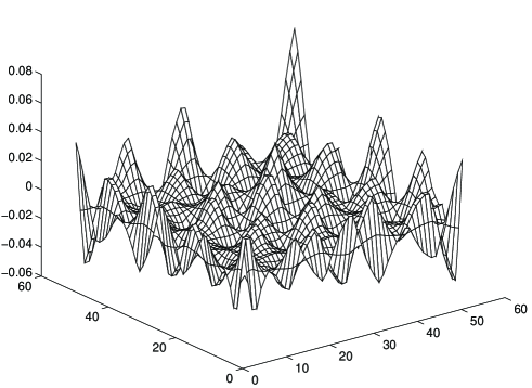
Figure 1: Localized two-dimensional partition.

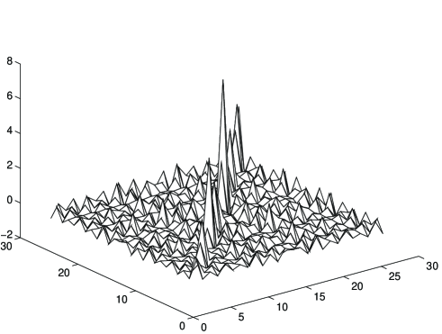
Figure 2: Metastable pattern.

Figure 3: Chaotic pattern.

Figure 4: Self-organization, step 1: towards confinement.

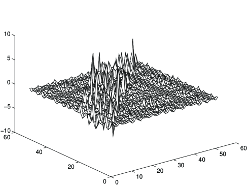
Figure 5: Self-organization, step 2: towards confinement.

Figure 6: Localized pattern(waveleton): energy confinement state.

References

- [1] A.N. Fedorova and M.G. Zeitlin, Math. and Comp. in Simulation, 46, 527 (1998); New Applications of Nonlinear and Chaotic Dynamics in Mechanics, Ed. F. Moon, (Kluwer, Boston, 1998) pp. 31-40, 101-108.
- [2] A.N. Fedorova and M.G. Zeitlin, in American Institute of Physics, Conf. Proc. 405 (1997), pp. 87-102; ”Nonlinear Dynamics of Accelerator via Wavelet Approach”, physics/9710035; 468 (1999), pp. 48-68, 69-93; ”Variational Approach in Wavelet Framework to Polynomial Approximations of Nonlinear Accelerator Problems”, physics/990262; ”Symmetry, Hamiltonian Problems and Wavelets in Accelerator Physics”, physics/990263.
- [3] A.N. Fedorova and M.G. Zeitlin, in The Physics of High Brightness Beams, Ed. J. Rosenzweig, 235, (World Scientific, Singapore, 2001) pp. 235-254; ”Variational- Wavelet Approach to RMS Envelope Equations”, physics/0003095.
- [4] A.N. Fedorova and M.G. Zeitlin, in Quantum Aspects of Beam Physics, Ed. P. Chen (World Scientific, Singapore, 2002) pp. 527-538, 539-550; ”Quasiclassical Calculations for Wigner Functions via Multiresolution”, physics/0101006; ”Localized Coherent Structures and Patterns Formation in Collective Models of Beam Motion”, physics/0101007.
- [5] A.N. Fedorova and M.G. Zeitlin, in Progress in Nonequilibrium Green’s Functions II, Ed. M. Bonitz, (World Scientific, 2003) pp. 481-492; ”BBGKY Dynamics: from Localization to Pattern Formation”, physics/0212066.
- [6] A.N. Fedorova and M.G. Zeitlin, in Quantum Aspects of Beam Physics, Eds. Pisin Chen, K. Reil (World Scientific, 2004) pp. 22-35; ”Pattern Formation in Wigner-like Equations via Multiresolution”, SLAC-R-630 and quant-phys/0306197; Nuclear Instruments and Methods in Physics Research Section A, 534, Issues 1-2, 309-313, 314 -318 (2004); ”Classical and Quantum Ensembles via Multiresolution. I. BBGKY Hierarchy”, quant- ph/0406009; ”Classical and Quantum Ensembles via Multiresolution. II. Wigner Ensembles”, quant-ph/0406010.
- [7] A.N. Fedorova and M.G. Zeitlin, Localization and Fusion Modeling in Plasma Physics. Part I: Math Framework for Non-Equilibrium Hierarchies, this volume.
- [8] R.C. Davidson and H. Qin, Physics of Intense Charged Particle Beams in High Energy Accelerators (World Scientific, Singapore, 2001); A.W. Chao, Physics of Collective Beam Instabilities in High Energy Accelerators (Wiley, New York, 1993). R. Balescu, Equilibrium and Nonequilibrium Statistical Mechanics, (Wiley, New York, 1975); C. Scovel, A. Weinstein, Comm. Pure. Appl. Math., 47, 683, 1994; H. Boozer, Rev. Mod. Phys., 76, 1071 (2004).
- [9] Y. Meyer, Wavelets and Operators (Cambridge Univ. Press, 1990); D. Donoho, WaveLab (Stanford, 2000).