IN PLASMA PHYSICS.

PART I: MATH FRAMEWORK FOR

NON-EQUILIBRIUM HIERARCHIES

Antonina N. Fedorova, Michael G. Zeitlin IPME RAS, St. Petersburg, V.O. Bolshoj pr., 61, 199178, Russia

e-mail: zeitlin@math.ipme.ru

e-mail: anton@math.ipme.ru

http://www.ipme.ru/zeitlin.html

http://www.ipme.nw.ru/zeitlin.html LOCALIZATION AND FUSION MODELING IN PLASMA PHYSICS. PART I: MATH FRAMEWORK FOR NON-EQUILIBRIUM HIERARCHIES Antonina  N. Fedorova and Michael  G. Zeitlin IPME RAS, Russian Academy of Sciences, V.O. Bolshoj pr., 61, 199178, St. Petersburg, Russia http://www.ipme.ru/zeitlin.html; http://www.ipme.nw.ru/zeitlin.html Abstract A fast and efficient numerical-analytical approach is proposed for description of complex behaviour in non-equilibrium ensembles in the BBGKY framework. We construct the multiscale representation for hierarchy of partition functions by means of the variational approach and multiresolution decomposition. Numerical modeling shows the creation of various internal structures from fundamental localized (eigen)modes. These patterns determine the behaviour of plasma. The localized pattern (waveleton) is a model for energy confinement state (fusion) in plasma. Abstract IN PLASMA PHYSICS. PART I: MATH FRAMEWORK FOR NON-EQUILIBRIUM HIERARCHIES Antonina N. Fedorova, Michael G. Zeitlin IPME RAS, St. Petersburg, V.O. Bolshoj pr., 61, 199178, Russia e-mail: zeitlin@math.ipme.ru e-mail: anton@math.ipme.ru http://www.ipme.ru/zeitlin.html http://www.ipme.nw.ru/zeitlin.html Two lectures presented at the Sixth Symposium on Current Trends in International Fusion Research, Washington D.C., March, 2005, edited by Emilio Panarella, NRC Reasearch Press, National Reasearch Council of Canada, Ottawa, Canada, 2006. BBGKY framework. We construct the multiscale representation for hierarchy of partition functions by means of the variational approach and multiresolution decomposition. Numerical modeling shows the creation of various internal structures from fundamental localized (eigen)modes. These patterns determine the behaviour of plasma. The localized pattern (waveleton) is a model for energy confinement state (fusion) in plasma. Two lectures presented at the Sixth Symposium on Current Trends in International Fusion Research, Washington D.C., March, 2005,

edited by Emilio Panarella, NRC Reasearch Press, National Reasearch Council of Canada, Ottawa, Canada, 2006.

BBGKY framework. We construct the multiscale representation for hierarchy of partition functions by means of the variational approach and multiresolution decomposition. Numerical modeling shows the creation of various internal structures from fundamental localized (eigen)modes. These patterns determine the behaviour of plasma. The localized pattern (waveleton) is a model for energy confinement state (fusion) in plasma.

be in thermodinamical equilibrium” Unknown author … Folklore

1 GENERAL INTRODUCTION

It is well known that fusion problem in plasma physics could be solved neither experimentally nor theoretically during last fifty years. At the same time, during this long period other areas of physics and engineering demonstrated vast growth, on the level of both theoretical understanding and practical smart realizability. We can only mention an unprecedent level of theoretical understanding in Quantum Field Theory and String Physics, as the top of this mountain, and solid state electronics penetrating in real life together with personal computers and a lot of related things. It should be mentioned that the former thing demanded and created a fantastic level of theoretical models and new beatiful mathematics while the latter depended only on the state of the art of engineers from Intel and other high-tech firms who created, e.g., the processor Pentium by means of the multiplication table (almost) only. Unfortunately, although plasma physics, as a whole, was a key source of the so called Soliton Theory (begining with numerical modeling by M. Kruskal and N. Zabusky), which was very important part of Mathematical Physics during twenty-five years, it itself used no advantage of these methods and approaches and created nothing comparable for a long time.

Because financing contributions in this area definitely exceeds that of almost all other areas of Physics, it seems that there are the serious obstacles which prevent real progress in the problem of real fusion as the main subject in the area. Of course, it may be a result of some unknown no-go theorem but it seems that the current theoretical level definitely demonstrates that not all possibilities, at least on the level of theoretical and matematical modeling, are exhausted. Surely, it is more than clear that perturbations, linearization, PIC or MC do not exhaust all instruments which we have at our hands on the route to theoretical understanding and predictions. Definitely, we need much more to have influence on almost free-of-theoretical-background work of experimentalists and engineers who contribute to ITER and other related top level projects.

So, this paper and related ones can be considered as a small contribution to an attempt to avoid the existing obstacles appeared on the main road of current plasma physics.

Definitely, the first thing which we need to change is a framework of generic mathematical methods which can only improve the current state of the theory.

Although, as in case of Pentium processors, there is a chance that engineers can solve all problems in a smart way without any theoretical contributions, but the current status of out-of-Science problems is such one that, definetely, we have no additional fifty years to wait when the appearance of fusion machines leads to total decreasing both the level of using of oil and the level of prices adequate for civilized countries.

So, after pointing out our vision of well known situation in the area, we will present some details of our attempts to change the standard approach [1], [2] to more proper one from our point of view [3]-[8].

Our postulates (conjectures) are as follows:

A) The fusion problem (at least at the first step) must be considered as a problem inside the (non) equilibrium ensemble in the full phase space. It means, at least, that:

A1) our dynamical variables are partitions (partition functions, hierarchy of N-point partition functions),

A2) it is impossible to fix a priori the concrete distribution function and postulate it (e.g. Maxwell-like or other concrete distributions) but, on the contrary, the proper distrubution(s) must be the solutions of proper (stochastic) dynamical problem(s), e.g., it may be the well-known framework of BBGKY hierarchy of kinetic equations or something similar. So, the full set of dynamical variables must include partitions also.

B) Fusion state = (meta) stable state (in the space of partitions on the whole phase space) in which most of energy of the system is concentrated in the relatively small area (preferable with measure zero) of the whole domain of definition in the phase space during the time period which is enough to take reasonable part of it outside for possible usage.

From the formal/mathematical point of view it means that:

B1) fusion state must be localized (first of all, in the phase space),

B2) we need a set of building blocks, localized basic states or eigenmodes which can provide

B3) the creation of localized pattern which can be considered as a possible model for plasma in a fusion state. Such pattern must be:

B4) (meta) stable and controllable because of obvious reasons.

So, in this paper our main courses are:

C1) to present smart localized building blocks which may be not only useful from point of view of analytical statements, such as the best possible localization, fast convergence, sparse operators representation, etc [9], but also exist as real physical fundamental modes,

C2) to construct various possible patterns with special attention to localized pattern which can be considered as a needful thing in analysis of fusion;

C3) after points C1 and C2 in ensemble (BBGKY) framework to consider some standard reductions to Vlasov-like and RMS-like equations (following the set-up from well-known results [2]) which may be useful also. These particular cases may be important as from physical point of view as some illustration of general consideration [10].

Sections 5 (Part I), and 1, 2 (Part II [10]) are more or less self-consistent, so potential readers may start from any of these Sections.

The lines above are motivated by our attempts to analyze the hidden internal contents of the phrase mentioned in the epigraph of this paper: “A magnetically confined plasma cannot be in thermodinamical equilibrium.” We guess that it is a well-known and well distributed fact. We found it, in particular, in the recent review paper [1]. Of course, the following is only a first order iteration on the long way to the main goal but we think that one needs to start from the right place to have some chance to reach the final point.

2 MOTIVATIONS: INTRODUCTION INTO MATHEMATICAL FRAMEWORK. KINDERGARTEN VERSION

It is obvious that any reasonable set-up for analysis of fusion leads to very complex system and one hardly believes that such system can be analyzed by means of almost exhausted methods like perturbations, linearization etc. At the same time, because such stochastic dynamics is overcompleted by short- and long-living fluctuations, instabilities, etc one needs to find something more proper than usual plane waves or gaussians for modeling a complicated complex behaviour. For reminiscences we may consider simple standard soliton equations like KdV, KP or sine-Gordon ones. It is well-known that neither linearization, nor perturbations, nor plane-wave-like approximations are proper for the reasonable analysis of such equations in contrary to wave or other simple linear equations: it is impossible to approximate the spectrum of such models (solitons, breathers or finite-gap solutions) by means of linear Fourier harmonics. They are not physical modes in complex situation. Moreover, such linear methods are not adequate in more complicated situation.

Below, we will give kindergarten-like introduction to our analytical framework. It would appear that as a first step in this direction is to find a reasonable extension of understanding of the non-equilibrium dynamics as a whole. One needs to sketch up the underlying ingredients of the theory (spaces of states, observables, measures, classes of smoothness, dynamical set-up etc) in an attempt to provide the maximally extendable but at the same time really calculable and realizable description of the complex dynamics inside hierarchies like BBKGY and their reductions. The general idea is rather simple: it is well known that the idea of “symmetry” is the key ingredient of any reasonable physical theory from classical (in)finite dimensional (integrable) Hamiltonian dynamics to different sub-planckian models based on strings (branes, orbifolds, etc). During the last century kinematical, dynamical and hidden symmetries played the key role in our understanding of physical process. Roughly speaking, the representation theory of underlying symmetry (classical or quantum, groups or (bi)algebras, finite or infinite dimensional, continuous or discrete) is a proper instrument for the description of proper (orbital) dynamics. A starting point for us is a possible model for fundamental localized mode with the subsequent description of the whole zoo of possible realizable (controllable) states/patterns which may be useful from the point of view of experimentalists and engineers. The proper representation theory is well known as “local nonlinear harmonic analysis”, in particular case of simple underlying symmetry-affine group-aka wavelet analysis. From our point of view the advantages of such approach are as follows:

i) natural realization of localized states in any proper functional realization of (functional) space of states,

ii) hidden symmetry of chosen realization of proper functional model provides the (whole) spectrum of possible states via the so-called multiresolution decomposition.

So, indeed, the hidden symmetry (non-abelian affine group in the simplest case) of the space of states via proper representation theory generates the physical spectrum and this procedure depends on the choice of the functional realization of the space of states. It explicitly demonstrates that the structure and properties of the functional realization of the space of states are the natural properties of physical world at the same level of importance as a particular choice of Hamiltonian, or the equation of motion, or the action principle (variational method).

At the next step we need to consider the consequences of our choice i), ii) for the algebra of operators. In this direction one needs to mention the class of operators we are interested in to present the proper description for a maximally generalized but reasonable class of problems. It seems that these must be pseudodifferential operators, especially if we underline that in the spirit of points i), ii) above we need to take Weyl framework for analyzing basic equations of motion. It is obvious, that the consideration of symbols of operators instead of operators themselves is the starting point as for the correct mathematical theory of pseudodifferential operators as for analysis of dynamics formulated in the language of symbols (Wigner-Weyl transform). In addition, it provides us by unified framework for analysis as classical problems as quantum ones.

It should be noted that in such picture we can naturally include the effects of self-interaction on the way of construction and subsequent analysis of nonlinear models. So, our consideration will be in the framework of (Nonlinear) Pseudodifferential Dynamics ($\Psi DOD$). As a result of i), ii), we will have:

iii) most sparse, almost diagonal, representation for a wide class of operators included in the set-up of the whole problems.

It is possible by using the so-called Fast Wavelet Transform representation for algebra of observables.

Then points i)-iii) provide us by

iv) natural (non-perturbative) multiscale decomposition for all dynamical quantities such as states, observables, partitions.

Existence of such internal multiscales with different dynamics at each scale and transitions, interactions, and intermittency between scales demonstrates that statistical mechanics in BBGKY form, despite its linear structure, is really a complicated problem from the mathematical point of view. It seems, that well-known underlying “stochastic” complexity is a result of transition by means of (still rather unclear) procedure of evolution from complexity related to individual classical dynamics to the rich pseudodifferential (more exactly, microlocal) structure on the non-equilibrium ensemble side.

We divide all possible configurations related to possible solutions of our kinetic hierarchies into two classes:

(a) standard solutions; (b) controllable solutions (solutions with prescribed qualitative type of behaviour).

Anyway, the whole zoo of solutions consists of possible patterns, including very important ones from the point of view of underlying physics:

v) localized modes (basis modes, eigenmodes) and chaotic (definitely, non proper for fusion modeling) or fusion-like localized patterns constructed from them.

It should be noted that these bases modes are nonlinear in contrast with usual ones because they come from (non) abelian generic group while the usual Fourier (commutative) analysis starts from $U(1)$ abelian modes (plane waves). They are really “eigenmodes” but in sense of decomposition of representation of the underlying hidden symmetry group which generates the multiresolution decomposition. The set of patterns is built from these modes by means of variational procedures more or less standard in mathematical physics. It allows to control the convergence from one side but, what is more important,

vi) to consider the problem of the control of patterns (types of behaviour) on the level of reduced (variational) algebraical equations.

We need to mention that it is possible to change the simplest generic group of hidden internal symmetry from the affine (translations and dilations) to much more general, but, in any case, this generic symmetry will produce the proper natural high localized eigenmodes, as well as the decomposition of the functional realization of space of states into the proper orbits; and all that allows to compute dynamical consequence of this procedure, i.e. pattern formation, and, as a result, to classify the whole spectrum of proper states.

For practical reasons controllable patterns (with prescribed behaviour) are the most useful. We mention the so-called waveleton-like pattern which we regard as the most important one. We use the following allusion in the space of words:

{waveleton}:={soliton} $\bigsqcup$ {wavelet}

It means:

vii) waveleton $\approx$ (meta)stable localized (controllable) pattern.

To summarize, the approach described below allows

viii) to solve wide classes of general $\Psi DOD$ problems, including generic for us BBGKY hierarchy and its reductions, and

ix) to present the analytical/numerical realization for physically interesting patterns, like fusion states.

We would like to emphasize the effectiveness of numerical realization of this program (minimal complexity of calculations) as additional advantage. So, items i)-ix) point out all main features of our approach [3]-[8].

2.1 Class of Models

Here we describe a class of problems which can be analyzed by methods described in the previous part. We start from individual dynamics and finish by (non)-equilibrium ensembles. Me mention here as classical models as quantum ones because both of them can be immersed in this unified framework and it is really motivated by “quantum-like” ideology.

All models belong to the $\Psi DOD$ class and can be described by a finite or infinite (named hierarchies in such cases) system of $\Psi DOD$ equations:

a) Individual classical/quantum mechanics ($cM/qM$): linear/nonlinear; $\{cM\}\subset\{qM\}$, $\ast$ - quantized for the class of polynomial Hamiltonians $H(p,q,t)=\sum_{i.j}a_{ij}(t)p^{i}q^{j}.$

An important generic example: Orbital motion (in Storage Rings). The magnetic vector potential of a magnet with $2n$ poles in Cartesian coordinates is

$$A=\sum_{n}K_{n}f_{n}(x,y),$$ (1)

where $f_{n}$ is a homogeneous function of $x$ and $y$ of order $n$. The cases $n=2$ to $n=5$ correspond to low-order multipoles: quadrupole, sextupole, octupole, decupole. The corresponding Hamiltonian is:

$$H(x,p_{x},y,p_{y},s) = \frac{p_{x}^{2}+p_{y}^{2}}{2}+\left(\frac{1}{\rho^{2}(s)}-k_{1}(s)\right)\cdot\frac{x^{2}}{2}+k_{1}(s)\frac{y^{2}}{2}$$ (2)

$$- {\cal R}e\left[\sum_{n\geq 2}\frac{k_{n}(s)+ij_{n}(s)}{(n+1)!}\cdot(x+iy)^{(n+1)}\right].$$

Terms corresponding to kick type contributions of rf-cavity:

$$A_{\tau}=-\frac{L}{2\pi k}\cdot V_{0}\cdot\cos\big{(}k\frac{2\pi}{L}\tau\big{)}\cdot\delta(s-s_{0})$$ (3)

or localized cavity with $V(s)=V_{0}\cdot\delta_{p}(s-s_{0})$ with $\delta_{p}(s-s_{0})=\sum^{n=+\infty}_{n=-\infty}\delta(s-(s_{0}+n\cdot L))$ at position $s_{0}$. The second example: using Serret-Frenet parametrization, after truncation of power series expansion of square root we have the following approximated (up to octupoles) Hamiltonian for orbital motion in machine coordinates:

$${\cal H} = \frac{1}{2}\cdot\frac{[p_{x}+H\cdot z]^{2}+[p_{z}-H\cdot x]^{2}}{[1+f(p_{\sigma})]}+p_{\sigma}-[1+K_{x}\cdot x+K_{z}\cdot z]\cdot f(p_{\sigma})$$

$$+ \frac{1}{2}\cdot[K_{x}^{2}+g]\cdot x^{2}+\frac{1}{2}\cdot[K_{z}^{2}-g]\cdot z^{2}-N\cdot xz+\frac{\lambda}{6}\cdot(x^{3}-3xz^{2})$$

$$+ \frac{\mu}{24}\cdot(z^{4}-6x^{2}z^{2}+x^{4})+\frac{1}{\beta_{0}^{2}}\cdot\frac{L}{2\pi\cdot h}\cdot\frac{eV(s)}{E_{0}}\cdot\cos\left[h\cdot\frac{2\pi}{L}\cdot\sigma+\varphi\right]$$

Then we use series expansion of function $f(p_{\sigma})$: $f(p_{\sigma})=f(0)+f^{\prime}(0)p_{\sigma}+f^{\prime\prime}(0)p_{\sigma}^{2}/2+\ldots=p_{\sigma}-p_{\sigma}^{2}/(2\gamma_{0}^{2})+\ldots$

and the corresponding expansion of RHS of equations. As a result, important models (2) and (4) belong to a class of polynomial Hamiltonians, generic for us class of individual dynamics.

b) QFT-like models in framework of the second quantization (dynamics in Fock spaces).

c) Classical (non) equilibrium ensembles via BBGKY Hierarchy (with reductions to different forms of Vlasov-Maxwell/Poisson equations).

d) Wignerization of a): Wigner-Moyal-Weyl-von Neumann-Lindblad.

e) Wignerization of c): Quantum (Non) Equilibrium Ensembles.

Important remarks: points a)-e) are considered in $\Psi DO$ picture of (Non)Linear $\Psi DO$ Dynamics (surely, all $qM\subset\Psi DOD$); dynamical variables/observables are the symbols of operators or functions; in case of ensembles, the main set of dynamical variables consists of partitions (n-particle partition functions).

2.2 Effects we are interested in

• Hierarchy of internal/hidden scales (time, space, phase space).

• Non-perturbative multiscales: from slow to fast contributions, from the coarser level of resolution/decomposition to the finer one.

• Coexistence of hierarchy of multiscale dynamics with transitions between scales.

• Realization of the key features of the complex nonequilibrium world such as the existence of chaotic and/or entangled (complex) states with possible destruction in some controllable regimes and transition to localized fusion-like states.

At this level we may interpret the effect of intermode interactions (in linear but pseudodifferential system!) as a result of simple interscale interaction or intermittency (with allusion to hydrodynamics), i.e. the mixing of orbits generated by multiresolution representation of hidden underlying symmetry. Surely, the concrete realization of such a symmetry is a natural physical property of the physical model as well as the space of representation and its proper functional realization.

One additional important comment: as usual in modern physics, we have the hierarchy of underlying symmetries; so our internal symmetry of functional realization of space of states is really not more than kinematical, because much more rich algebraic structure, related to operator Cuntz algebra and quantum groups, is hidden inside. The proper representations can generate much more interesting effects than ones described above. We will consider it elsewhere but mention here only how it can be realized by the existing functorial maps between proper categories:

{QMF} $\longrightarrow$ Loop groups $\longrightarrow$ Cuntz operator algebra $\longrightarrow$ Quantum Group structure, where {QMF} are the so-called quadratic mirror filters generating the realization of multiresolution decomposition/representation in any functional space; loop group is well known in many areas of physics, e.g. soliton theory, strings etc, roughly speaking, its algebra coincides with Virasoro algebra; Cuntz operator algebra is universal $C^{*}$ algebra generated by N elements with two relations between them; Quantum group structure (bialgebra, Hopf algebra, etc) is well known in many areas because of its universality. It should be noted the appearance of natural Fock structure inside this functorial sequence above with the creation operator realized as some generalization of Cuntz-Toeplitz isometries. Surely, all that can open a new vision of old problems and bring new possibilities.

We finish this part by the following qualitative definitions of key objects (patterns). Their description and understanding in various physical models is our main goal in this direction.

• By localized states (localized modes) we mean the building blocks for solutions or generating modes which are localized in maximally small region of the phase (as in c- as in q-case) space.

• By a chaotic pattern we mean some solution (or asymptotics of solution) which has random-like distributed energy spectrum in the full domain of definition.

• By a localized pattern (waveleton) we mean (asymptotically) (meta) stable solution localized in a relatively small region of the whole phase space (or a domain of definition). In this case the energy is distributed during some time (sufficiently large) between only a few localized modes (from point 1). We believe it to be a good model for plasma in fusion state (energy confinement).

2.3 Methods

• Representation theory of internal/hidden/underlying symmetry, Kinematical, Dynamical, Hidden.

• Arena (space of representation): proper functional realization of (Hilbert) space of states.

• Harmonic analysis on (non)abelian group of internal symmetry. Local Nonlinear (non-abelian) Harmonic Analysis (e.g, wavelet/gabor etc. analysis) instead of linear non-localized U(1) Fourier analysis. Multiresolution (multiscale) representation. Dynamics on proper orbit/scale (inside the whole hierarchy of multiscales) in functional space. The key ingredients are the appearance of multiscales (orbits) and the existence of high-localized natural (eigen)modes [9].

• Variational formulation (control of convergence, reductions to algebraic systems, control of type of behaviour).

3 SET-UP/FORMULATION

Let us consider the following generic $\Psi DOD$ dynamical problem

$$L^{j}\{Op^{i}\}\Psi=0,$$ (5)

described by a finite or infinite number of equations which include general classes of operators $Op^{i}$ such as differential, integral, pseudodifferential etc

Surely, all hierarchies and their reductions are inside this class.

The main objects are:

• (Hilbert) space of states, $H=\{\Psi\}$, with a proper functional realization, e.g.,: $L^{2}$, Sobolev, Schwartz, $C^{0}$, $C^{k}$, … $C^{\infty}$, …; definitely, $L^{2}(R^{2})$, $L^{2}(S^{2})$, $L^{2}(S^{1}\times S^{1})$, $L^{2}(S^{1}\times S^{1}\ltimes Z_{n})$ are different objects proper for different physics inside. E.g., two last cases describe tokamak and stellarator, correspondingly. Of course, they are different spaces and generate different physics.

• Class of smoothness. The proper choice determines natural consideration of dynamics with/without Chaos/Fractality property.

• Decompositions

  $$\Psi\approx\sum_{i}a_{i}e^{i}$$ (6)

  via high-localized bases (wavelet families, generic wavelet packets etc), frames, atomic decomposition (Fig.  1) with the following main properties: (exp) control of convergence, maximal rate of convergence for any $\Psi$ in any $H$ [9].

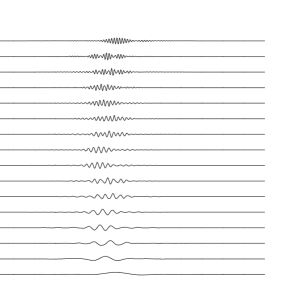
  Figure 1: Localized modes.

• Observables/Operators (ODO, PDO, $\Psi DO$ , SIO,…, Microlocal analysis of Kashiwara-Shapira (with change from functions to sheafs)) satisfy the main property - the matrix representation in localized bases

  $$<\Psi|Op^{i}|\Psi>$$ (7)

  is maximum sparse:

  $$\left(\begin{array}[]{cccc}D_{11}&0&0&\ldots\\ 0&D_{22}&0&\ldots\\ 0&0&D_{33}&\ldots\\ \vdots&\vdots&\vdots&\ddots\end{array}\right).$$

  This almost diagonal structure is provided by the so-called Fast Wavelet Transform [9].

• Measures: multifractal wavelet measures $\{\mu_{i}\}$ together with the class of smoothness are very important for analysis of complicated analytical behaviour [9].

• Variational/Projection methods, from Galerkin to Rabinowitz minimax, Floer (in symplectic case of Arnold-Weinstein curves with preservation of Poisson or symplectic structures). Main advantages are the reduction to algebraic systems, which provides a tool for the smart subsequent control of behaviour and control of convergence.

• Multiresolution or multiscale decomposition, $MRA$ (or wavelet microscope) consists of the understanding and choosing of (internal) symmetry structure, e.g., affine group = {translations, dilations} or many others; construction of representation/action of this symmetry on $H=\{\Psi\}$.

  As a result of such hidden coherence together with using point vi) we’ll have:

  • LOCALIZED BASES

  • EXACT MULTISCALE DECOMPOSITION

  with the best convergence properties and real evaluation of the rate of convergence via proper “multi-norms”.

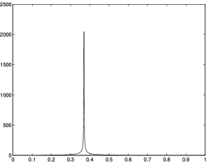
Figure 2: Kick.

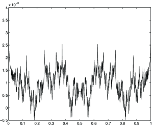
Figure 4: RW-fractal.

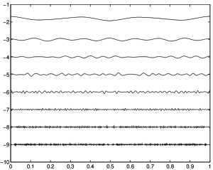
Figure 7: MRA for RW-fractal.

  Figure  2, 3, 5, 6 demonstrate MRA decompositions for one- and multi-kicks while Figures 4 and 7 present the same for the case of the generic simple fractal model, Riemann-Weierstrass function [9].

• Effectiveness of proper numerics: CPU-time, HDD-space, minimal complexity of algorithms, and (Shannon) entropy of calculations are provided by points i)-vii) above.

• Quantization via $\ast$ star product or Deformation Quantization. It was considered elsewhere [8].

Finally, such Variational-Multiscale approach based on points i)-ix) provides us by the full ZOO of PATTERNS: LOCALIZED, CHAOTIC, etc.

In next Sections we will consider details for important case of kinetic equations.

We present the explicit analytical construction for solutions of BBGKY hierarchy, which is based on tensor algebra extensions of multiresolution representation for states, observables, partitions and variational formulation. We give explicit representation for hierarchy of n-particle reduced distribution functions in the base of high-localized generalized coherent (regarding underlying generic symmetry (affine group in the simplest case)) states given by polynomial tensor algebra of our basis functions (wavelet families, wavelet packets), which takes into account contributions from all underlying hidden multiscales from the coarsest scale of resolution to the finest one to provide full information about dynamical process. In some sense, our approach for ensembles (hierarchies) resembles Bogolyubov’s one and related approaches but we don’t use any perturbation technique (like virial expansion) or linearization procedures. Most important, that numerical modeling in all cases shows the creation of different internal (coherent) structures from localized modes, which are related to stable (equilibrium) or unstable type of behaviour and corresponding pattern (waveletons) formation.

4 INTRODUCTION INTO PHYSICAL MOTIVES

So, we will consider the application of our numerical/analytical technique based on local nonlinear harmonic analysis approach for the description of complex non-equilibrium behaviour of statistical ensembles, considered in the framework of the general BBGKY hierarchy of kinetic equations and their different truncations/reductions. The main points of our ideology are described below. All these facts are well-known or described above but it is preferable to bring it together to present our arguments in more clear form.

• Kinetic theory is an important part of general statistical physics related to phenomena which cannot be understood on the thermodynamic or fluid models level.

• We restrict ourselves to the rational/polynomial type of nonlinearities (with respect to the set of all dynamical variables, including partitions) that allows to use our results, based on the so called multiresolution framework and the variational formulation of initial nonlinear (pseudodifferential) problems.

• Our approach is based on the set of mathematical methods which give a possibility to work with well-localized bases in functional spaces and provide the maximum sparse forms for the general type of operators (differential, integral, pseudodifferential) in such bases.

• It provides the best possible rates of convergence and minimal complexity of algorithms inside and, as a result, saves CPU time and HDD space.

• In all cases below by the system under consideration we mean the full BBGKY hierarchy or some its cut-off or its various reductions. Our scheme of cut-off for the infinite system of equations is based on some criterion of convergence of the full solution by means of some norm introduced in the proper functional space constructed by us.

• This criterion is based on a natural norm in the proper functional space, which takes into account (non-perturbatively) the underlying multiscale structure of complex statistical dynamics. According to our approach the choice of the underlying functional space is important to understand the corresponding complex dynamics.

• It is obvious that we need accurately to fix the space, where we construct the solutions, evaluate convergence etc. and where the very complicated infinite set of operators, appeared in the BBGKY formulation, acts.

• We underline that many concrete features of the complex dynamics are related not only to the concrete form/class of operators/equations but depend also on the proper choice of function spaces, where operators act. It should be noted that the class of smoothness (related at least to the appearance of chaotic/fractal-like type of behaviour) of the proper functional space under consideration plays a key role in the following.

• At this stage our main goal is an attempt of classification and construction of a possible zoo of nontrivial (meta) stable states/patterns: high-localized (nonlinear) eigenmodes, complex (chaotic-like or entangled) patterns, localized (stable) patterns (waveletons). We will use it later for fusion description, modeling and control.

• Localized (meta)stable pattern (waveleton) is a good image for fusion state in plasma (energy confinement).

Our constructions can be applied to the following general individual (members of ensemble under consideration) Hamiltonians:

$$H_{N}=\sum^{N}_{i=1}\Big{(}\frac{p^{2}_{i}}{2m}+U_{i}(q)\Big{)}+\sum_{1\leq i\leq j\leq N}U_{ij}(q_{i},q_{j}),$$ (8)

where the potentials $U_{i}(q)=U_{i}(q_{1},\dots,q_{N})$ and $U_{ij}(q_{i},q_{j})$ are restricted to rational functions on the coordinates. Let $L_{s}$ and $L_{ij}$ be the Liouvillean operators and

$$F_{N}(x_{1},\dots,x_{N};t)$$ (9)

be the hierarchy of $N$-particle distribution function, satisfying the standard BBGKY hierarchy ($\upsilon$ is the volume):

$$\frac{\partial F_{s}}{\partial t}+L_{s}F_{s}=\frac{1}{\upsilon}\int d\mu_{s+1}\sum^{s}_{i=1}L_{i,s+1}F_{s+1}.$$ (10)

Our key point is the proper nonperturbative generalization of the previous perturbative multiscale approaches. The infinite hierarchy of distribution functions is:

$$F=\{F_{0},F_{1}(x_{1};t),\dots,F_{N}(x_{1},\dots,x_{N};t),\dots\},$$ (11)

where

$$F_{p}(x_{1},\dots,x_{p};t)\in H^{p},$$ (12)

$$H^{0}=R,\quad H^{p}=L^{2}(R^{6p}),\quad F\in H^{\infty}=H^{0}\oplus H^{1}\oplus\dots\oplus H^{p}\oplus\dots$$

with the natural Fock space like norm (guaranteeing the positivity of the full measure):

$$(F,F)=F^{2}_{0}+\sum_{i}\int F^{2}_{i}(x_{1},\dots,x_{i};t)\prod^{i}_{\ell=1}\mu_{\ell}.$$ (13)

• Multiresolution decomposition naturally and efficiently introduces the infinite sequence of the underlying hidden scales, which is a sequence of increasing closed subspaces $V_{j}\in L^{2}(R)$:

  $$...V_{-2}\subset V_{-1}\subset V_{0}\subset V_{1}\subset V_{2}\subset...$$ (14)

• Our variational approach reduces the initial problem to the problem of solution of functional equations at the first stage and some algebraic problems at the second one. As a result, the solutions of the (truncated) hierarchies have the following multiscale decomposition via high-localized eigenmodes ($\omega_{l}\sim 2^{l}$, $k^{s}_{m}\sim 2^{m}$)

  $$F(t,x_{1},x_{2},\dots) = \sum_{(i,j)\in Z^{2}}a_{ij}U^{i}\otimes V^{j}(t,x_{1},\dots),$$ (15)

  $$V^{j}(t) = V_{N}^{j,slow}(t)+\sum_{l\geq N}V^{j}_{l}(\omega_{l}t),$$

  $$U^{i}(x_{s}) = U_{M}^{i,slow}(x_{s})+\sum_{m\geq M}U^{i}_{m}(k^{s}_{m}x_{s}),$$

  which corresponds to the full multiresolution expansion in all underlying time/space scales.

• In this way one obtains contributions to the full solution from each scale of resolution or each time/space scale or from each nonlinear eigenmode.

• It should be noted that such representations give the best possible localization properties in the corresponding (phase) space/time coordinates.

• Numerical calculations are based on compactly supported wavelets and related wavelet families and on evaluation of the accuracy on the level $N$ of the corresponding cut-off of the full system w.r.t. the norm above.

• Numerical modeling shows the creation of different internal structures from localized modes, which are related to (meta)stable or unstable type of behaviour and the corresponding patterns (waveletons) formation. Reduced algebraic structure provides the pure algebraic control of stability/unstability scenario.

• As a final point we will consider the construction for

  CONTROLLABLE (META) STABLE WAVELETON CONFIGURATION REPRESENTING A REASONABLE APRROXIMATION FOR THE REALIZABLE CONFINEMENT STATE.

5 BBGKY HIERARCHY

We start from set-up for kinetic BBGKY hierarchy and present explicit analytical construction for solutions of hierarchy of equations, which is based on tensor algebra extensions of multiresolution representation and variational formulation. We give explicit representation for hierarchy of n-particle reduced distribution functions in the base of high-localized generalized coherent (w.r.t. underlying affine group) states given by polynomial tensor algebra of wavelets, which takes into account contributions from all underlying hidden multiscales from the coarsest scale of resolution to the finest one to provide full information about stochastic dynamical process.

Let $M$ be the phase space of ensemble of $N$ particles (${\rm dim}M=6N$) with coordinates

$$x_{i}=(q_{i},p_{i}),\quad i=1,...,N,\quad q_{i}=(q^{1}_{i},q^{2}_{i},q^{3}_{i})\in R^{3},$$ (16)

$$p_{i}=(p^{1}_{i},p^{2}_{i},p^{3}_{i})\in R^{3},q=(q_{1},\dots,q_{N})\in R^{3N}.$$

Individual and collective measures are:

$$\mu_{i}=\mathrm{d}x_{i}=\mathrm{d}q_{i}p_{i},\quad\mu=\prod^{N}_{i=1}\mu_{i}.$$ (17)

Distribution function

$$D_{N}(x_{1},\dots,x_{N};t)$$ (18)

satisfies Liouville equation of motion for ensemble with Hamiltonian $H_{N}$ :

$$\frac{\partial D_{N}}{\partial t}=\{H_{N},D_{N}\}$$ (19)

and normalization constraint

$$\int D_{N}(x_{1},\dots,x_{N};t)\mathrm{d}\mu=1,$$ (20)

where Poisson brackets are:

$$\{H_{N},D_{N}\}=\sum^{N}_{i=1}\Big{(}\frac{\partial H_{N}}{\partial q_{i}}\frac{\partial D_{N}}{\partial p_{i}}-\frac{\partial H_{N}}{\partial p_{i}}\frac{\partial D_{N}}{\partial q_{i}}\Big{)}.$$ (21)

Our constructions can be applied to the following general Hamiltonians:

$$H_{N}=\sum^{N}_{i=1}\Big{(}\frac{p^{2}_{i}}{2m}+U_{i}(q)\Big{)}+\sum_{1\leq i\leq j\leq N}U_{ij}(q_{i},q_{j}),$$ (22)

where potentials

$$U_{i}(q)=U_{i}(q_{1},\dots,q_{N})$$ (23)

and

$$U_{ij}(q_{i},q_{j})$$ (24)

are not more than rational functions on coordinates. Let $L_{s}$ and $L_{ij}$ be the Liouvillean operators (vector fields)

$$L_{s} = \sum^{s}_{j=1}\Big{(}\frac{p_{j}}{m}\frac{\partial}{\partial q_{j}}-\frac{\partial u_{j}}{\partial q}\frac{\partial}{\partial p_{j}}\Big{)}-\sum_{1\leq i\ leqj\leq s}L_{ij},$$ (25)

$$L_{ij} = \frac{\partial U_{ij}}{\partial q_{i}}\frac{\partial}{\partial p_{i}}+\frac{\partial U_{ij}}{\partial q_{j}}\frac{\partial}{\partial p_{j}}.$$ (26)

For $s=N$ we have the following representation for Liouvillean vector field

$$L_{N}=\{H_{N},\cdot\}$$ (27)

and the corresponding equation of motion for ensemble:

$$\frac{\partial D_{N}}{\partial t}+L_{N}D_{N}=0$$ (28)

$L_{N}$ is a self-adjoint operator w.r.t. standard pairing on the set of phase space functions. Let

$$F_{N}(x_{1},\dots,x_{N};t)=\sum_{S_{N}}D_{N}(x_{1},\dots,x_{N};t)$$ (29)

be the N-particle distribution function ($S_{N}$ is permutation group of $N$ elements). Then we have the hierarchy of reduced distribution functions ($V^{s}$ is the corresponding normalized volume factor)

$$F_{s}(x_{1},\dots,x_{s};t)=V^{s}\int D_{N}(x_{1},\dots,x_{N};t)\prod_{s+1\leq i\leq N}\mu_{i}.$$ (30)

After standard manipulations we arrive to BBGKY hierarchy:

$$\frac{\partial F_{s}}{\partial t}+L_{s}F_{s}=\frac{1}{\upsilon}\int\mathrm{d}\mu_{s+1}\sum^{s}_{i=1}L_{i,s+1}F_{s+1}.$$ (31)

It should be noted that we may apply our approach even to more general formulation.

For s=1,2 we have:

$$\frac{\partial F_{1}(x_{1};t)}{\partial t}+\frac{p_{1}}{m}\frac{\partial}{\partial q_{1}}F_{1}(x_{1};t)=\frac{1}{\upsilon}\int\mathrm{d}x_{2}L_{12}F_{2}(x_{1},x_{2};t)\frac{\partial F_{2}(x_{1},x_{2};t)}{\partial t}+$$ (32)

$$\Big{(}\frac{p_{1}}{m}\frac{\partial}{\partial q_{1}}+\frac{p_{2}}{m}\frac{\partial}{\partial q_{2}}-L_{12}\Big{)}\cdot F_{2}(x_{1},x_{2};t)=\frac{1}{\upsilon}\int\mathrm{d}x_{3}(L_{13}+L_{23})F_{3}(x_{1},x_{2};t)$$

As in the general situation as in particular ones (cut-off, e.g.) we are interested in the cases when

$$F_{k}(x_{1},\dots,x_{k};t)=\prod^{k}_{i=1}F_{1}(x_{i};t)+G_{k}(x_{1},\dots,x_{k};t),$$ (33)

where $G_{k}$ are correlators, really have additional reductions as in the simplest case of one-particle Vlasov/Boltzmann-like systems. Then by using such physical motivated reductions or/and during the corresponding cut-off procedure we obtain instead of linear and pseudodifferential (in general case) equations their finite-dimensional but nonlinear approximations with the polynomial type of nonlinearities (more exactly, multilinearities). Our key point in the following consideration is the proper generalization of naive perturbative multiscale Bogolyubov’s structure.

6 MULTISCALE ANALYSIS

The infinite hierarchy of distribution functions satisfying BBGKY system in the thermodynamical limit is:

$$F=\{F_{0},F_{1}(x_{1};t),F_{2}(x_{1},x_{2};t),\dots,\quad F_{N}(x_{1},\dots,x_{N};t),\dots\},$$ (34)

where

$$F_{p}(x_{1},\dots,x_{p};t)\in H^{p},\quad H^{0}=R,\quad H^{p}=L^{2}(R^{6p})$$ (35)

(or any different proper functional space),

$$F\in H^{\infty}=H^{0}\oplus H^{1}\oplus\dots\oplus H^{p}\oplus\dots$$ (36)

with the natural Fock-space like norm (of course, we keep in mind the positivity of the full measure):

$$(F,F)=F^{2}_{0}+\sum_{i}\int F^{2}_{i}(x_{1},\dots,x_{i};t)\prod^{i}_{\ell=1}\mu_{\ell}$$ (37)

while in particular case

$$F_{k}(x_{1},\dots,x_{k};t)=\prod^{k}_{i=1}F_{1}(x_{i};t)$$ (38)

First of all we consider $F=F(t)$ as function of the time variable only, $F\in L^{2}(R)$, via multiresolution decomposition which naturally and efficiently introduces the infinite sequence of underlying hidden scales into the game.

Because affine group of translations and dilations is inside the approach, this method resembles the action of a microscope. We have contribution to final result from each scale of resolution from the whole infinite scale of spaces.

Let the closed subspace $V_{j}(j\in{\bf Z})$ correspond to level $j$ of resolution, or to scale $j$. We consider a multiresolution analysis of $L^{2}(R)$ (of course, we may consider any different functional space) which is a sequence of increasing closed subspaces $V_{j}$ [9]:

$$...V_{-2}\subset V_{-1}\subset V_{0}\subset V_{1}\subset V_{2}\subset...$$ (39)

satisfying the following properties: let $W_{j}$ be the orthonormal complement of $V_{j}$ with respect to $V_{j+1}$:

$$V_{j+1}=V_{j}\bigoplus W_{j}$$ (40)

then we have the following decomposition:

$$\{F(t)\}=\bigoplus_{-\infty<j<\infty}W_{j}$$ (41)

or in case when $V_{0}$ is the coarsest scale of resolution:

$$\{F(t)\}=\overline{V_{0}\displaystyle\bigoplus^{\infty}_{j=0}W_{j}}.$$ (42)

Subgroup of translations generates basis for fixed scale number:

$${\rm span}_{k\in Z}\{2^{j/2}\Psi(2^{j}t-k)\}=W_{j}.$$ (43)

The whole basis is generated by action of full affine group:

$${\rm span}_{k\in Z,j\in Z}\{2^{j/2}\Psi(2^{j}t-k)\}={\rm span}_{k,j\in Z}\{\Psi_{j,k}\}=\{F(t)\}.$$ (44)

Let sequence

$$\{V_{j}^{t}\},V_{j}^{t}\subset L^{2}(R)$$ (45)

correspond to multiresolution analysis on time axis,

$$\{V_{j}^{x_{i}}\}$$ (46)

correspond to multiresolution analysis for coordinate $x_{i}$, then

$$V_{j}^{n+1}=V^{x_{1}}_{j}\otimes\dots\otimes V^{x_{n}}_{j}\otimes V^{t}_{j}$$ (47)

corresponds to multiresolution analysis for n-particle distribution function $F_{n}(x_{1},\dots,x_{n};t)$. E.g., for $n=2$:

$$V^{2}_{0}=\{f:f(x_{1},x_{2})=\sum_{k_{1},k_{2}}a_{k_{1},k_{2}}\phi^{2}(x_{1}-k_{1},x_{2}-k_{2}),\qquad a_{k_{1},k_{2}}\in\ell^{2}(Z^{2})\},$$ (48)

where

$$\phi^{2}(x_{1},x_{2})=\phi^{1}(x_{1})\phi^{2}(x_{2})=\phi^{1}\otimes\phi^{2}(x_{1},x_{2}),$$ (49)

and $\phi^{i}(x_{i})\equiv\phi(x_{i})$ form a multiresolution basis corresponding to $\{V_{j}^{x_{i}}\}$. If

$$\{\phi^{1}(x_{1}-\ell)\},\ \ell\in Z$$ (50)

form an orthonormal set, then

$$\phi^{2}(x_{1}-k_{1},x_{2}-k_{2})$$ (51)

form an orthonormal basis for $V^{2}_{0}$. Action of affine group provides us by multiresolution representation of $L^{2}(R^{2})$. After introducing detail spaces $W^{2}_{j}$, we have, e.g.

$$V^{2}_{1}=V^{2}_{0}\oplus W^{2}_{0}.$$ (52)

Then 3-component basis for $W^{2}_{0}$ is generated by translations of three functions

$$\Psi^{2}_{1}=\phi^{1}(x_{1})\otimes\Psi^{2}(x_{2}),$$ (53)

$$\Psi^{2}_{2}=\Psi^{1}(x_{1})\otimes\phi^{2}(x_{2}),$$

$$\Psi^{2}_{3}=\Psi^{1}(x_{1})\otimes\Psi^{2}(x_{2})$$

Also, we may use the rectangle lattice of scales and one-dimentional wavelet decomposition:

$$f(x_{1},x_{2})=\sum_{i,\ell;j,k}<f,\Psi_{i,\ell}\otimes\Psi_{j,k}>\Psi_{j,\ell}\otimes\Psi_{j,k}(x_{1},x_{2}),$$ (54)

where bases functions

$$\Psi_{i,\ell}\otimes\Psi_{j,k}$$ (55)

depend on two scales $2^{-i}$ and $2^{-j}$ [9].

We obtain our multiscale/multiresolution representations below via the variational wavelet approach for the following formal representation of the BBGKY system (or its finite-dimensional nonlinear approximation for the $n$-particle distribution functions) with the corresponding obvious constraints on the distribution functions.

7 VARIATIONAL APPROACH

Let $L$ be an arbitrary (non)linear differential/integral operator with matrix dimension $d$ (finite or infinite), which acts on some set of functions from $L^{2}(\Omega^{\otimes^{n}})$: $\quad\Psi\equiv\Psi(t,x_{1},x_{2},\dots)=\Big{(}\Psi^{1}(t,x_{1},x_{2},\dots),\dots$, $\Psi^{d}(t,x_{1},x_{2},\dots)\Big{)}$, $\quad x_{i}\in\Omega\subset{\bf R}^{6}$, $n$ is the number of particles:

$$L\Psi \equiv L(Q,t,x_{i})\Psi(t,x_{i})=0,$$ (56)

$$Q \equiv Q_{d_{0},d_{1},d_{2},\dots}(t,x_{1},x_{2},\dots,\partial/\partial t,\partial/\partial x_{1},\partial/\partial x_{2},\dots,\int\mu_{k})=$$

$$= \sum_{i_{0},i_{1},i_{2},\dots=1}^{d_{0},d_{1},d_{2},\dots}q_{i_{0}i_{1}i_{2}\dots}(t,x_{1},x_{2},\dots)\Big{(}\frac{\partial}{\partial t}\Big{)}^{i_{0}}\Big{(}\frac{\partial}{\partial x_{1}}\Big{)}^{i_{1}}\Big{(}\frac{\partial}{\partial x_{2}}\Big{)}^{i_{2}}\dots\int\mu_{k}.$$

Let us consider now the $N$ mode approximation for the solution as the following ansatz:

$$\Psi^{N}(t,x_{1},x_{2},\dots)=\sum^{N}_{i_{0},i_{1},i_{2},\dots=1}a_{i_{0}i_{1}i_{2}\dots}A_{i_{0}}\otimes B_{i_{1}}\otimes C_{i_{2}}\dots(t,x_{1},x_{2},\dots).$$ (57)

We shall determine the expansion coefficients from the following conditions (different related variational approaches are considered also):

$$\ell^{N}_{k_{0},k_{1},k_{2},\dots}\equiv\int(L\Psi^{N})A_{k_{0}}(t)B_{k_{1}}(x_{1})C_{k_{2}}(x_{2})\mathrm{d}t\mathrm{d}x_{1}\mathrm{d}x_{2}\dots=0.$$ (58)

Thus, we have exactly $dN^{n}$ algebraical equations for $dN^{n}$ unknowns $a_{i_{0},i_{1},\dots}$. This variational approach reduces the initial problem to the problem of solution of functional equations at the first stage and some algebraical problems at the second. We consider the multiresolution expansion as the second main part of our construction. The solution is parametrized by the solutions of two sets of reduced algebraical problems, one is linear or nonlinear (depending on the structure of the operator $L$) and the rest are linear problems related to the computation of the coefficients of the algebraic equations. These coefficients can be found by some methods by using the compactly supported wavelet basis functions.

As a result the solution has the following multiscale/multiresolution decomposition via nonlinear high-localized eigenmodes

$$F(t,x_{1},x_{2},\dots) = \sum_{(i,j)\in Z^{2}}a_{ij}U^{i}\otimes V^{j}(t,x_{1},x_{2},\dots),$$ (59)

$$V^{j}(t) = V_{N}^{j,slow}(t)+\sum_{l\geq N}V^{j}_{l}(\omega_{l}t),\quad\omega_{l}\sim 2^{l},$$

$$U^{i}(x_{s}) = U_{M}^{i,slow}(x_{s})+\sum_{m\geq M}U^{i}_{m}(k^{s}_{m}x_{s}),\quad k^{s}_{m}\sim 2^{m},$$

which corresponds to the full multiresolution expansion in all underlying time/space scales. These formulae give the expansion into a slow and fast oscillating parts. So, we may move from the coarse scales of resolution to the finest ones for obtaining more detailed information about the dynamical process. In this way we give contribution to our full solution from each scale of resolution or each time/space scale or from each nonlinear eigenmode. It should be noted that such representations give the best possible localization properties in the corresponding (phase)space/time coordinates. In contrast with different approaches our formulae do not use perturbation technique or linearization procedures. Numerical calculations are based on compactly supported wavelets and related wavelet families and on evaluation of the accuracy regarding norm (37):

$$\|F^{N+1}-F^{N}\|\leq\varepsilon$$ (60)

8 MODELING OF PATTERNS

To summarize, the key points are:

1. The ansatz-oriented choice of the (multidimensional) bases related to some polynomial tensor algebra.

2. The choice of proper variational principle. A few projection or Galerkin-like principles for constructing (weak) solutions are considered. The advantages of formulations related to biorthogonal (wavelet) decomposition should be noted.

3. The choice of bases functions in the scale spaces $W_{j}$ from wavelet zoo. They correspond to high-localized (nonlinear) oscillations/excitations, nontrivial local (stable) distributions/fluctuations, etc. Besides fast convergence properties it should be noted minimal complexity of all underlying calculations, especially in case of choice of wavelet packets which minimize Shannon entropy.

4. Operator representations providing maximum sparse representations for arbitrary (pseudo) differential/ integral operators: $\quad\mathrm{d}f/\mathrm{d}x$, $\mathrm{d}^{n}f/\mathrm{d}x^{n}$, $\int T(x,y)f(y)\mathrm{d}y$, etc [9].

5. (Multi)linearization. Besides the variation approach we can consider also a different method to deal with (polynomial) nonlinearities: para-products-like decompositions [9].

Formulae (57), (59) provide, in principle, a fast convergent decomposition for the general solutions of the systems (31), (32), (56) in terms of contributions from all underlying hidden internal scales. Of course, we cannot guarantee that each concrete system (32) with fixed coefficients will have a priori a specific type of behaviour, either localized or chaotic. Instead, we can analyze whether such typical structures described by qualitative definitions from Section 2.2. really appear.

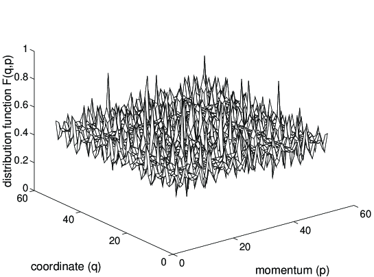
Figure 10: Chaotic partition.

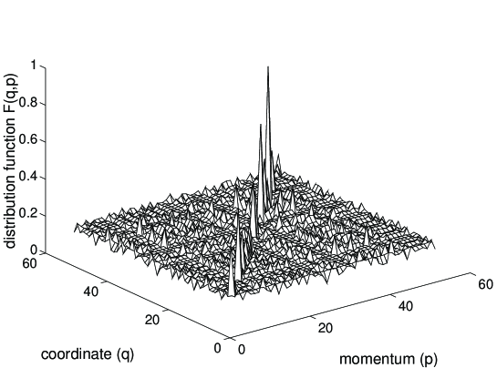
Figure 11: Localized partition.

To classify the qualitative behaviour we apply standard methods from general control theory or really use the control. We start from a priori unknown coefficients, the exact values of which will subsequently be recovered. Roughly speaking, we fix only class of nonlinearity (polynomial in our case) which covers a broad variety of examples of possible truncation of the systems. As a simple model we choose band-triangular non-sparse matrices $(a_{ij})$ in particular case $d=2$. These matrices provide tensor structure of bases in (extended) phase space and are generated by the roots of the reduced variational (Galerkin-like) systems. As a second step we need to restore the coefficients from these matrices by which we may classify the types of behaviour. We start with the two-dimensional localized base eigenmode (Fig. 9, d=2), which was constructed as a tensor product of the two localized one-dimensional modes (Fig. 8, d=1). Fig. 10, corresponding to chaotic pattern, presents the result of summation of series up to value of the dilation/scale parameter equal to six on the bases of symmlets with the corresponding matrix elements equal to one. The size of matrix is 512x512 and as a result we provide modeling for one-particle distribution function corresponding to standard Vlasov-like cut-off with $F_{2}=F_{1}^{2}$. So, different possible distributions of the root values of the generic algebraical system (58) provide qualitatively different types of behaviour. The above choice provides us by a distribution with chaotic-like equidistribution. But, if we consider a band-like structure of matrix $(a_{ij})$ with the band along the main diagonal with finite size ($\ll 512$) and values, e.g. five, while the other values are equal to one, we obtain localization in a fixed finite area of the full phase space, i.e. almost all energy of the system is concentrated in this small volume. This corresponds to waveleton case and is shown in Fig. 11, constructed by means of Daubechies-based wavelet packets. Depending on the type of solution, such localization may be present during the whole time evolution (asymptotically-stable) or up to the needed value on time scale, e.g., enough for plasma fusion/confinement.

Now we discuss how to solve the inverse/synthesis problem or how to restore the coefficients of the initial systems (31), (32). Let

$$L^{0}(Q^{0})\Psi^{0}=0$$ (61)

be the system (56) with the fixed coefficients $Q^{0}$. The corresponding solution $\Psi^{0}$ is represented by formulae (57) or (59), which are parametrized by roots of reduced algebraic system (58) and constructed by some choice of the tensor product bases from Section 6. The proper counterpart of the system (61) with prescribed behaviour $\Psi^{u}$, corresponding to a given choice of both tensor product structure and coefficients $\{a_{ij}\}$ described above, corresponds to the class of systems like (56) but with undetermined coefficients $Q^{u}$ and has the same form

$$L^{u}(Q^{u})\Psi^{u}=0.$$ (62)

Our goal is to restore coefficients $Q^{u}$ from (61), (62) and explicit representations for solutions $\Psi^{0}$ and $\Psi^{u}$. This is a standard problem in the adaptive control theory: one adds a controlling signal $u(x,t)$ which deforms the controlled signal $\Psi(x,t)$ from the fixed state $\Psi^{0}(x,t)$ to the prescribed one $\Psi^{u}(x,t)$. At the same time one can determine the parameters $Q^{u}$ [3]. Finally, we apply two variational constructions. The first one gives the systems of algebraic equations for unknown coefficients, generated by the following set of functionals

$$\Phi_{N}=\int\Big{(}(L^{0}-L^{u})\Psi^{u}_{N},\Psi^{0}_{N}\Big{)}{\rm d}\mu_{N},$$ (63)

where $N$ means the $N$-order approximation according to formulae (57). The unknown parameters $Q^{*}$ are given by $Q^{*}=\lim_{N\to\infty}Q^{u}_{N}$. The second is an important additional constraint on the region $\mu_{0}$ in the phase space where we are interested in localization of almost all energy $E=\int H(\Psi^{u}){\rm d}\mu$, where $E$ is the proper energy Marsden-like functional [2].

We believe that the appearance of nontrivial localized (meta) stable patterns observed by these methods is a general effect which present in the full BBGKY-hierarchy, due to its complicated intrinsic multiscale dynamics and it depends on neither the cut-off level nor the phenomenological-like hypothesis on correlators. So, representations for solutions like (59) and as a result the prediction of the existence of the (asymptotically) stable localized patterns/states (waveletons) which can realize energy confinement (fusion) states in BBGKY-like systems are the main results of this approach. In addition, lines above in this Section open way to solve the control problem by means of reduction from initial (pseudodifferential) formulation to reduced set of algebraic one (58) and as a result to create and support the needed fusion state(s).

9 CONCLUSIONS

Let us summarize our main results:

• Physical Conjectures:

• P1

  State of fusion (confinement of energy) in plasma physics may and need be considered from the point of view of non-equilibrium statistical physics. According to this BBGKY framework looks naturally as first iteration. Main dynamical variables are partitions.

• P2

  High localized nonlinear eigenmodes (Figures 1, 8, 9) are real physical modes important for fusion modeling. Intermode multiscale interactions create various patterns from these fundamental building blocks, and determine the behaviour of plasma.

  High localized (meta) stable patterns (waveletons), considered as long-living fluctuations, are proper images for plasma in fusion state (Figures 12, 13).

• Mathematical framework:

• M1 Problems under consideration, like BBGKY hierarchies (31) or their reductions (32) and (3)-(5), (20), (21), (26) from part II [10] are considered as $\Psi DO$ problems in the framework of proper family of methods unified by effective multiresolution approach.

• M2

  Formulae (59) based on generalized dispersion relations (GDR) (58) provide exact multiscale representation for all dynamical variables (partitions, first of all) in the basis of high-localized nonlinear (eigen)modes. Numerical realizations in this framework are maximally effective from the point of view of complexity of all algorithms inside. GDR provide the way for the state control on the algbraic level.

• Realizability

  According to this approach, it is possible on formal level, in principle, to control ensemble behaviour and to realize the localization of energy (confinement state) inside the waveleton configurations created from a few fundamentals modes only (Figures 14, 15).

• Open Questions

• Q1

  Definitely, all above is only very naive ensemble approach. Current level of non-equilibrium statistical physics provides us only by BBGKY generic framework. All related internal problems are well-known but we still have nothing better. At the same time possible Vlasov-like reductions or phenomenological models also look as very far from reasonable from the point of view of the fusion problem set-up.

• Q2

  Considering for allusion successful areas of physics like superconductivity, for example, we may conclude that only microscopic BCS formulation provides the full explanation although Ginzburg-Landau (GL) phenomenological approach and even Froelich’s and London’s ones contributed to the general picture. Whether Vlasov equations are the analogue of GL ones and whether it is possible to construct microscopic model for plasma, these two important questions remain unanswered at present time.

• Q3

  It may be natural also that approaches proposed in this paper and related ones are wrong because the proper and adequate framework for solution of fusion problem is related to confinement of magnetic lines or loops (new physical dynamical variables instead of partitions) or fluxes instead of confinement of localized point modes (attribute of any local field theory) considered as new and really proper physical variables. Such approach demands the topological background related to proper mathematical constructions. As allusion it is possible to consider the description of (fractional) quantum Hall effect by means of Chern-Simons/anyon models which allow to describe the dynamics on (of) knots and braids analytically. Anyway, it is still possible to apply successfull methods from (M1) and (M2) here too. Remarks in Section 2.2. demonstrate interesting relations. Other open possibility is related to taking into account internal quantum properties. From this point of view our approach is very useful because we unify quantum description and its classical counterpart in the general $\Psi DO$ framework.

10 ACKNOWLEDGEMENTS

We are very grateful to Professors E. Panarella (Chairman of the Steering Committee), R. Kirkpatrick (LANL) and R.E.H. Clark, G. Mank and his Colleagues from IAEA (Vienna) for their help, support and kind attention before, during and after 6th Symposium on Fusion Research (March 2005, Washington, D.C.). We are grateful to Dr. A.G. Sergeyev for his permanent support in problems related to hard- and software.

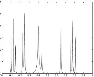
Figure 3: Multi-Kicks.

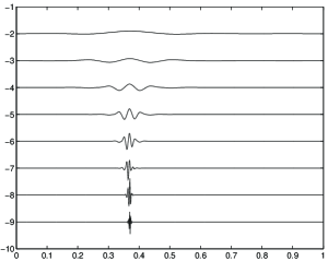
Figure 5: MRA for Kick.

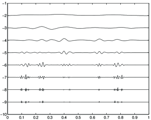
Figure 6: MRA for Multi-Kicks.

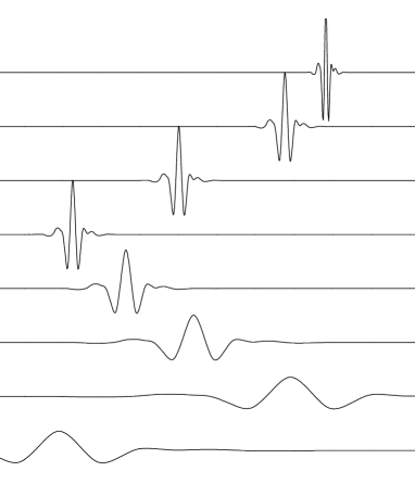
Figure 8: Localized one-dimensional modes.

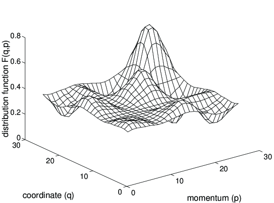
Figure 9: Localized mode contribution to distribution function.

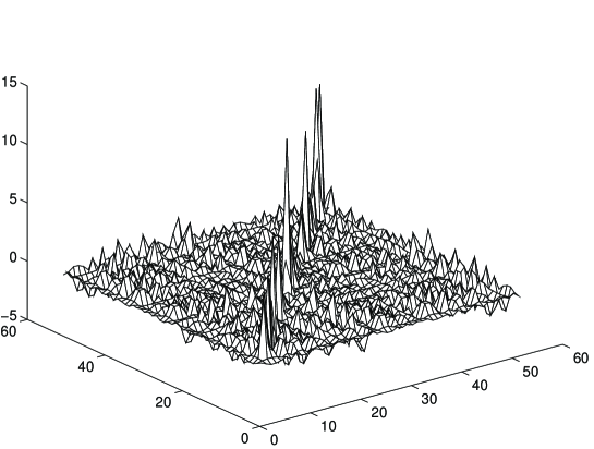
Figure 12: Fusion-like state.

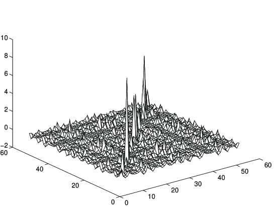
Figure 13: Fusion-like state: waveleton mode.

Figure 14: Fusion-like state.

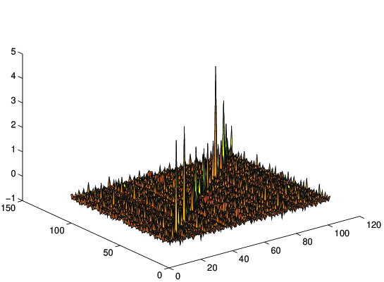
Figure 15: Fusion-like state.

References

- [1] A. H. Boozer, Rev. Mod. Phys., 76, 1071 (2004).
- [2] R.C. Davidson and H. Qin, Physics of Intense Charged Particle Beams in High Energy Accelerators (World Scientific, Singapore, 2001); A.W. Chao, Physics of Collective Beam Instabilities in High Energy Accelerators (Wiley, New York, 1993). R. Balescu, Equilibrium and Nonequilibrium Statistical Mechanics, (Wiley, New York, 1975); C. Scovel, A. Weinstein, Comm. Pure. Appl. Math., 47, 683, 1994.
- [3] A.N. Fedorova and M.G. Zeitlin, Math. and Comp. in Simulation, 46, 527 (1998); New Applications of Nonlinear and Chaotic Dynamics in Mechanics, Ed. F. Moon, (Kluwer, Boston, 1998) pp. 31-40, 101-108.
- [4] A.N. Fedorova and M.G. Zeitlin, in American Institute of Physics, Conf. Proc. 405 (1997), pp. 87-102; “Nonlinear Dynamics of Accelerator via Wavelet Approach”, physics/9710035; 468 (1999), pp. 48-68, 69-93; “Variational Approach in Wavelet Framework to Polynomial Approximations of Nonlinear Accelerator Problems”, physics/990262; “Symmetry, Hamiltonian Problems and Wavelets in Accelerator Physics”, physics/990263.
- [5] A.N. Fedorova and M.G. Zeitlin, in The Physics of High Brightness Beams, Ed. J. Rosenzweig, 235, (World Scientific, Singapore, 2001) pp. 235-254; “Variational-Wavelet Approach to RMS Envelope Equations”, physics/0003095.
- [6] A.N. Fedorova and M.G. Zeitlin, in Quantum Aspects of Beam Physics, Ed. P. Chen (World Scientific, Singapore, 2002) pp. 527-538, 539-550; “Quasiclassical Calculations for Wigner Functions via Multiresolution”, physics/0101006; “Localized Coherent Structures and Patterns Formation in Collective Models of Beam Motion”, physics/0101007.
- [7] A.N. Fedorova and M.G. Zeitlin, in Progress in Nonequilibrium Green’s Functions II, Ed. M. Bonitz, (World Scientific, 2003) pp. 481-492; “BBGKY Dynamics: from Localization to Pattern Formation“, physics/0212066.
- [8] A.N. Fedorova and M.G. Zeitlin, in Quantum Aspects of Beam Physics, Eds. Pisin Chen, K. Reil (World Scientific, 2004) pp. 22-35; “Pattern Formation in Wigner-like Equations via Multiresolution”, SLAC-R-630 and quant-phys/0306197; Nuclear Instruments and Methods in Physics Research Section A, 534, Issues 1-2, 309-313, 314 -318 (2004); “Classical and Quantum Ensembles via Multiresolution. I. BBGKY Hierarchy”, quant-ph/0406009; “Classical and Quantum Ensembles via Multiresolution. II. Wigner Ensembles”, quant-ph/0406010.
- [9] Y. Meyer, Wavelets and Operators (Cambridge Univ. Press, 1990); D. Donoho, WaveLab (Stanford, 2000)
- [10] A.N. Fedorova and M.G. Zeitlin, Localization and Fusion Modeling in Plasma Physics. Part II: Vlasov-like Systems. Important Reductions, this volume.