Analytic calculation of energies and wave functions of the quartic and pure quartic oscillators

Abstract

Ground state energies and wave functions of quartic and pure quartic oscillators are calculated by first casting the Schrödinger equation into a nonlinear Riccati form and then solving that nonlinear equation analytically in the first iteration of the quasilinearization method (QLM). In the QLM the nonlinear differential equation is solved by approximating the nonlinear terms by a sequence of linear expressions. The QLM is iterative but not perturbative and gives stable solutions to nonlinear problems without depending on the existence of a smallness parameter. Our explicit analytic results are then compared with exact numerical and also with WKB solutions and it is found that our ground state wave functions, using a range of small to large coupling constants, yield a precision of between 0.1 and 1 percent and are more accurate than WKB solutions by two to three orders of magnitude. In addition, our QLM wave functions are devoid of unphysical turning point singularities and thus allow one to make analytical estimates of how variation of the oscillator parameters affects physical systems that can be described by the quartic and pure quartic oscillators.

I Introduction

A basic nonrelativistic quantum mechanics problem is to solve the Schrödinger equation with a potential $V(x)$ that governs motion of a given physical system. The first two terms of the power expansion of a one-dimensional, even potential around an equilibrium position are

$$\frac{g^{2}x^{2}}{2}+\lambda x^{4},$$ (1)

where $x$ is the deviation from an equilibrium position. The above potential describes the dynamics of a great many systems that deviate from the idealized picture of pure harmonic motion. When both $g$ and $\lambda$ are nonzero, we call this potential a “quartic” or quartic anharmonic oscillator; whereas, when $g=0$ with nonzero $\lambda$ it is dubbed a “pure quartic” oscillator. In addition to providing an excellent description of spectroscopic molecular vibrational data(see Ref.Laane and references therein), the quartic anharmonic oscillator (1) also serves as a basic tool for checking various approximate and perturbative methods in quantum mechanics. Such an application appears in several recent field theoretical model studies Zam ; Cas ; Muel ; Alva ; Path ; Chil ; Chen ; Zap ; Gil ; Jaf ; AHS ; AAP ; Dus .

It is well known Ben ; Sim that for the quartic anharmonic oscillator the perturbation expansion diverges even for small couplings and becomes completely useless for strong coupling. In view of this divergence of perturbation theory, we have adopted KM2 ; KMT the general and very powerful quasilinearization method (QLM) K ; BK ; VBM1 ; MT ; VBM2 , which although iterative is not a perturbative method. In QLM the $p$-th order solution of a nonlinear differential equation with N variables is obtained by first approximating the nonlinear aspect by a sequence of linear terms and then iteratively solving the associated linear equations. This iterative process converges to a solution without requiring the existence of a smallness parameter. Properties and applications of the quasilinearization method were reviewed recently in VBM3 .

To apply the quasilinearization method, one first casts the Schrödinger equation into the nonlinear Riccati form and then solves that nonlinear equation by the QLM iterations. In a series of publications KM2 ; KMT ; KMT1 ; KM3 ; KM4 , we have shown that for a range of anharmonic and other physical potentials (with both weak and strong couplings), the QLM iterates display very fast quadratic convergence. Indeed, after just a few QLM iterations, energies and wave functions are obtained with extremely high accuracy, reaching 20 significant figures for the energy of the sixth iterate even in the case of very large coupling constants.

Although numerical solutions using either the QLM or direct numerical solution of the differential equations can be very accurate, it is important to also provide analytic solutions. Analytic solutions allow one to gauge the role of different potential parameters, and explore the influence of such variations on the properties of the quantum system under study. However, in contrast to the harmonic oscillator, the anharmonic oscillator cannot be solved analytically, and thus one usually has to resort to approximations.

The goal of this paper is to obtain and test approximate analytic solutions for the quartic and pure quartic oscillators using the explicit analytic equation for the first QLM iterate. We will show that both energies and wave functions will be represented by closed analytic expressions with the accuracy of the wave functions being between 0.1 and 1 percent for both small and large coupling constants. Various accurate analytic expressions for the energies have already appeared in the literature based on using convergent, strong coupling expansions generated by rearrangement of the usual divergent weak coupling expansion Jan or by some variational requirement Math . However, accurate analytic expressions representing wave functions have not hitherto been known. That result is provided here.

II Main formulae

The usual WKB substitution $y(x)=\frac{\psi^{\prime}(x)}{\psi(x)}$ converts the Schrödinger equation to the nonlinear Riccati form

$$\frac{dy(x)}{dx}+\left[k^{2}(x)+y^{2}(x)\right]=0.$$ (2)

Here $k^{2}(x)=2\left[E-V(x)\right]$, where we use $m=1,\hbar=1$ units. The quasilinearization VBM1 ; VBM2 ; MT ; VBM3 of Eq.(2) leads to the recurrence differential equation

$$\frac{dy_{p}(x)}{dx}+(2y_{p-1}(x))y_{p}(x)=y_{p-1}^{2}(x)-k^{2}(x),$$ (3)

where $y_{p}(x)$ is the subsequent $p^{th}$ QLM iterate, which have the same boundary condition as $y(x)$ of Eq.(2). Note that Eq.(3) is a linear equation of the form $\frac{dy_{p}(x)}{dx}+f(x)y_{p}(x)=q(x),$ with $f(x)=2y_{p-1}(x)$ and $q(x)=y_{p-1}^{2}(x)-k^{2}(x).$

Let us use Eqs.(3) to estimate the ground state wave function and energy of the quartic oscillator. Excited states will be considered elsewhere.

The ground state wave function is nodeless and for an even potential (1) should therefore be an even function. Its logarithmic derivative is necessarily odd, and therefore the boundary condition obviously is $y(0)=0$ and correspondingly $y_{p}(0)=0.$

II.1 Linear Initial Condition

The zero iterate should be based on physical considerations. Let us consider first an initial guess $y_{0}(x)=-gx$. This linear initial condition completely neglects the anharmonic term containing $\lambda$ compared with the harmonic term and thus this initial guess is expected to be reasonable only for relatively small values of $\lambda$.

Solution of the first order linear differential Eq.(3) with the above zero boundary condition at the origin can always be found analytically. For $p=1$ the solution is

$$y_{1}(x)=2\,e^{gx^{2}}\int_{0}^{x}e^{-gs^{2}}(g^{2}s^{2}+\lambda s^{4}-E_{1})\,ds.$$ (4)

Integration by parts, yields an expression for $y_{1}(x)$ that involves the error function ${\rm Erf}(x)\equiv\frac{2}{\pi}\int_{0}^{x}e^{-t^{2}}dt$:

$$y_{1}(x) = \frac{1}{4g^{5/2}}\{-2x\sqrt{g}\ (2g^{3}+3\lambda+2g\lambda x^{2})$$

$$+ e^{gx^{2}}\sqrt{\pi}\ {\rm Erf}(x\sqrt{g})\ [2g^{2}(g-2E_{1})+3\lambda]\ \,\}.$$

The asymptotic expression ${\rm Erf}(x)\simeq(1-\frac{e^{-x^{2}}}{\sqrt{\pi}x})$ for $|x|\rightarrow\infty$,  indicates that $y_{1}(x)$ will be exponentially large for very large $x$ unless the second term in Eq.(LABEL:eq:ig2) is made zero. Correspondingly, invoking the condition $2g^{2}(g-2E_{1})+3\lambda=0$ yields the energy and the logarithmic derivative in the first iteration: $E_{1}=\frac{a}{2}$ and $y_{1}(x)=-ax-bx^{3}$, where $a=g+\frac{3\lambda}{2g^{2}};\,\,\,b=\frac{\lambda}{g}$. This leads to the first QLM iteration wave function $\psi(x)=C\exp{\left[-\frac{gx^{2}}{2}-\lambda\left(\frac{3x^{2}}{4g^{2}}+\frac{x^{4}}{4g}\right)\right]}$. This QLM result for the energy coincides with the perturbative result, as well as with the result obtained by Friedberg, Lee and Zhao FL who used their recently developed iterative method for solving the Schrödinger equation.

The wave functions we obtained above obviously have incorrect asymptotic behavior. Also, the energies $E_{1}$ calculated for different $\lambda,$ as displayed in Table 1, are far from being precise. Therefore, to improve the result one is tempted to go to the second QLM iteration, using $y_{1}(x)$ as an input.

Eq.(3) then yields the second iterate

$$y_{2}(x) = e^{ax^{2}+\frac{b}{2}x^{4}}\int_{0}^{x}\{[a^{2}+g^{2}+2(ab+\lambda)t^{2}$$

$$+ b^{2}t^{4}]t^{2}-2E_{2}\}e^{-at^{2}-\frac{b}{2}t^{4}}dt.$$

Since $y_{2}(x)e^{-(ax^{2}+\frac{b}{2}x^{4}})$ approaches a constant when $x$ goes to infinity, $y_{2}(x)$ and consequently the corresponding wave function grows exponentially at infinity, unless the integral in Eq.(II.1) equals zero when its upper limit equals infinity. This condition yields the following expression for the energy $E_{2}$ in the second iteration:

$$E_{2}=\frac{\int_{0}^{\infty}\left[a^{2}+g^{2}+2\left(ab+\lambda\right)t^{2}+b^{2}t^{4}\right]t^{2}e^{-at^{2}-\frac{b}{2}t^{4}}dt}{2\int_{0}^{\infty}e^{-at^{2}-\frac{b}{2}t^{4}}dt}.$$ (7)

Values of $E_{2},$ for this initial linear form, are compared to exact values $E$ calculated numerically in Table 1. It is seen that $E_{2}$ approximates the exact $E$ reasonably well only for small $\lambda,$ as we anticipated would result from using an initial linear condition. We now turn to another choice for the initial form.

II.2 Quadratic Initial Condition

To ensure a proper wave function asymptotically, one needs an adequate initial guess. Our second condition is based on the asymptotic behavior of the quartic potential. The zeroth iterate of the logarithmic derivative, $y_{0}(x),$ is for example now obtained by taking an initial iterate of quadratic form $y_{0}(x)=-\sqrt{2\lambda}\ x^{2}.$ This choice for the first iterate automatically satisfies the asymptotic and $x=0$ boundary conditions, but is based on neglecting the harmonic term compare with the anharmonic one.

With this quadratic initial condition, the solution $y_{1}(x)$ of Eq.(3) satisfying $y_{1}(0)=0$ is then given by

$$y_{1}(x)=e^{\frac{2}{3}\sqrt{2\lambda}\ x^{3}}\int_{0}^{x}e^{-\frac{2}{3}\sqrt{2\lambda}\ s^{3}}\left[4\lambda\ s^{4}+g^{2}s^{2}-2E_{1}\right]ds.$$ (8)

Note, that $y_{1}(x)e^{-\frac{2}{3}\sqrt{2\lambda}\ x^{3}}$ approaches a constant, $C_{\infty},$ as $x$ goes to infinity, and consequently $y_{1}(x)$ grows exponentially at infinity unless the above limit $C_{\infty},$ is set to zero. The latter condition yields another expression for the energy based on the quadratic initial condition:

$$E_{1}=\frac{\int_{0}^{\infty}e^{-\frac{2}{3}\sqrt{2\lambda}\ s^{3}}\left[2\lambda\ s^{4}+\frac{g^{2}s^{2}}{2}\right]ds}{\int_{0}^{\infty}e^{-\frac{2}{3}\sqrt{2\lambda}\ s^{3}}ds}.$$ (9)

The integrals in Eq.(9) can be expressed in terms of the Euler Gamma function $\Gamma(x)$ GR . The final expression for the first iterate energy based on a quadratic initial condition reads

$$E_{1}=\frac{\lambda^{\frac{1}{6}}}{3^{\frac{1}{3}}\Gamma\left(\frac{1}{3}\right)}\left[\frac{3g^{2}}{4\sqrt{\lambda}}+\lambda^{\frac{1}{6}}3^{\frac{2}{3}}\Gamma\left(\frac{2}{3}\right)\right].$$ (10)

This result should be proper for large $\lambda$ when the second term of the quartic potential $\frac{g^{2}x^{2}}{2}+\lambda x^{4}$ dominates over the harmonic term and thus a term containing $g$ in initial guess $y_{0}(x)$ could be neglected. The above expression for the energy is not expected to be suitable for small $\lambda$. Indeed, one can see that for the $\lambda\rightarrow 0,$ the energy in Eq.(10) diverges.

II.3 Linear Plus Quadratic Initial Condition

To obtain a result accommodating arbitrary values of both $g$ and $\lambda,$ one has to start from an initial choice $y_{0}(x)$ that takes into account the asymptotic behavior of both the harmonic and the anharmonic parts of the potential. Let us choose, for example, $y_{0}(x)=-gx-\sqrt{2\lambda}x^{2}$ which is a linear combination of our two previous initial guesses. This yields

$$y_{1}(x) = 2e^{gx^{2}+\frac{2\sqrt{2\lambda}}{3}x^{3}}\int_{0}^{x}[t^{2}\left(g^{2}+g\sqrt{2\lambda}t+2\lambda t^{2}\right)$$ (11)

$$- E_{1}]e^{-gt^{2}-\frac{2\sqrt{2\lambda}}{3}t^{3}}dt,$$

with

$$E_{1}=\frac{\int_{0}^{\infty}t^{2}\left(g^{2}+g\sqrt{2\lambda}t+2\lambda t^{2}\right)e^{-gt^{2}-\frac{2\sqrt{2\lambda}}{3}t^{3}}dt}{\int_{0}^{\infty}e^{-gt^{2}-\frac{2\sqrt{2\lambda}}{3}t^{3}}dt}.$$ (12)

Another possible initial guess, which also accounts for the asymptotic behavior of both harmonic and anharmonic parts of the potential is $y_{0}(x)=-\sqrt{g^{2}x^{2}+2\lambda x^{4}}$. This guess is easy to justify by assuming that $y^{\prime}(x)$ in Eq.(2) at large $x$ becomes negligible compare with $y^{2}(x)$ and therefore $y^{2}(x)$ can be set equal $k^{2}(x)=g^{2}x^{2}+2\lambda x^{4}-2E\approx g^{2}x^{2}+2\lambda x^{4}$ since in this expression we can neglect $E$ for sufficiently large $x$.

The solution of Eq.(3) using the initial condition $y_{0}(x)=-\sqrt{g^{2}x^{2}+2\lambda x^{4}},$ is only slightly more complicated than in when one uses the initial guess $y_{0}(x)=-gx-\sqrt{2\lambda}x^{2},$ and is given by the expression

$$y_{1}(x)=2e^{\frac{(g^{2}+2\lambda x^{2})^{\frac{3}{2}}}{3\lambda}}\int_{0}^{x}e^{-\frac{(g^{2}+2\lambda t^{2})^{\frac{3}{2}}}{3\lambda}}\left[g^{2}t^{2}+2\lambda t^{4}-E_{1}\right]dt.$$ (13)

The condition to avoid exponential behavior of the logarithmic derivative at infinity now yields the following expression for the ground state energy

$$E_{1}=\frac{\int_{0}^{\infty}t^{2}\left(g^{2}+2\lambda t^{2}\right)e^{-\frac{(g^{2}+2\lambda t^{2})^{\frac{3}{2}}}{3\lambda}}dt}{\int_{0}^{\infty}e^{-\frac{(g^{2}+2\lambda t^{2})^{\frac{3}{2}}}{3\lambda}}dt}.$$ (14)

For a pure quartic oscillator with $g=0,$ both Eqs.(11) and (13) reduce to

$$y_{1}(x)=2e^{\frac{2\sqrt{2\lambda}x^{3}}{3}}\int_{0}^{x}e^{-\frac{2\sqrt{2\lambda}t^{3}}{3}}\left[2\lambda t^{4}-E_{1}\right]dt$$ (15)

with $E_{1}$ given by

$$E_{1}=\frac{2\lambda\int_{0}^{\infty}e^{-\frac{2\sqrt{2\lambda}}{3}s^{3}}s^{4}ds}{\int_{0}^{\infty}e^{-\frac{2\sqrt{2\lambda}}{3}s^{3}}ds}=\lambda^{\frac{1}{3}}3^{\frac{1}{3}}\frac{\Gamma\left(\frac{2}{3}\right)}{\Gamma\left(\frac{1}{3}\right)}\simeq 0.729011\lambda^{\frac{1}{3}}.$$ (16)

In view of Eq.(16) $y_{1}(x)$ of Eq.(15) can be expressed in terms of a special function,; namely, the Exponential Integral GR ${\textbf{EI}}_{\mu}(z)=\int_{1}^{\infty}e^{-zt}t^{-\mu}dt$:

$$y_{1}(x) = -\sqrt{2\lambda}\,x^{2}+\frac{2}{3}e^{\frac{2\sqrt{2\lambda}}{3}x^{3}}\{-\sqrt{2\lambda}\,x^{2}{\textbf{EI}}_{\frac{1}{3}}\left(\frac{2\sqrt{2\lambda}}{3}x^{3}\right)$$ (17)

$$+ \lambda^{\frac{1}{3}}3^{\frac{1}{3}}\frac{\Gamma(\frac{2}{3})}{\Gamma(\frac{1}{3})}x\,{\textbf{EI}}_{\frac{2}{3}}\left(\frac{2\sqrt{2\lambda}}{3}x^{3}\right)\}.$$

This expression for the log derivative yields a first iterate QLM wave function, based on the initial condition $y_{0}(x)=-\sqrt{g^{2}x^{2}+2\lambda x^{4}},$ that is the main result of our paper.

The exact dependence of $E_{1}$ on $\lambda$ for the pure quartic oscillator has the same form, but with a factor of $0.667\,986\,259$ before $\lambda^{\frac{1}{3}}$ Jan , so that the accuracy of the QLM prediction for the energy is about 9.1 percent. The WKB energy can be easily estimated and gives $E_{WKB}\simeq 0.546267\lambda^{\frac{1}{3}}$, an accuracy of 18.2 percent.

Table 1: Ground state energies $E$ for the quartic oscillator potential $U(x)=g^{2}x^{2}/2+\lambda x^{4}$ with $g=1$.

$\lambda$	$E_{exact}$	$E_{WKB}$	$\Delta E_{WKB}$	$E^{(1)}$	$\Delta E^{(1)}$	$E^{(2)};y_{0}=-gx$	$\Delta E^{(2)}$	$E^{(3)}$	$\Delta E^{(3)}$	$E^{(4)}$	$\Delta E^{(4)}$	$E^{(3)};$ $y_{0}=$	$\Delta E^{(3)}$
				$y_{0}=-gx$	(%)	$2^{nd}iteration$	(%)	$y_{0}=-x^{2}\sqrt{2\lambda}$	(%)	$y_{0}=-gx-x^{2}\sqrt{2\lambda}$	(%)	$-\sqrt{g^{2}x^{2}+2\lambda x^{4}}$	(%)
0	1/2	1/2	0	1/2	0	1/2	0			1/2	0	1/2	0
0.1	0.55915	0.53328	4.6	0.575	2.8	0.55983	0.1	0.75658	35	0.56940	1.8	0.56149	0.4
0.3	0.63799	0.58466	8.3	0.725	13.6	0.64869	1.7	0.77799	21.9	0.64838	1.6	0.64705	1.4
0.5	0.69618	0.62538	10.2	0.875	25.7	0.72728	4.4	0.82319	18.2	0.70552	1.3	0.71126	2.2
1	0.80377	0.70420	12.4	1.25	55.5	0.91423	13.7	0.92313	14.8	0.81138	0.95	0.83090	3.4
2	0.95157	0.81667	14.2	2	110	1.2829	34.8	1.07257	12.7	0.95853	0.73	0.99577	4.6
10	1.50497	1.25412	16.7	8		4.2628	183	1.6607	10.3	1.5259	1.4	1.61085	7.0
100	3.13138	2.57181	17.9	75.5				3.4256	9.4	3.2564	4.0	3.40039	8.5
1000	6.69422	5.47955	18.1	750.5				7.3095	9.2	7.1171	6.3	7.29744	9.0

III Results and discussion

The ground state energies for the quartic oscillator in the first QLM approximation for different initial guesses and for values of $g=1$ and $\lambda$ between zero and one thousand and their comparison with the numerically calculated exact and WKB values are given in Table 1. One can see that the values computed using explicit equations (12) and (14) for the QLM energy are significantly more accurate than the WKB values or than values obtained in the first and second QLM iterations with the initial guess $y_{0}(x)=-gx$. They have a precision of 0.4 to 9 percent for values of $\lambda$ varying between 0.1 and 1000, respectively.

However, the main results of our work, are not the expressions for the energy. As mentioned in the introduction, such expressions were already given in different forms by others. Our major results are the analytic expressions for the wave functions given by Eqs.(11) and Eq.(13), which are based on using the first QLM iterate with the initial conditions $y_{0}=-gx-\sqrt{2\lambda}x^{2}$ and $y_{0}=-\sqrt{g^{2}x^{2}+2\lambda x^{4}}$, respectively.

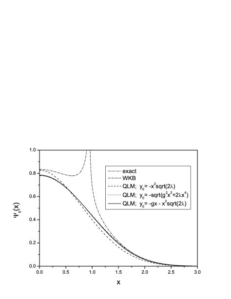
Figure 1: Comparison of the WKB, QLM and exact wave functions for the ground state of the quartic oscillator for $g=1,\lambda=0.1$.

Figure 2: Logarithm of the differences of the WKB and QLM wave functions with exact wave function for the ground state of the quartic oscillator for $g=1,\lambda=0.1.$

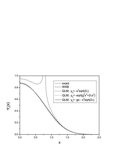
Figure 3: Comparison of the WKB, QLM and exact wave functions for the ground state of the quartic oscillator for $g=1,\lambda=1$.

Figure 4: Logarithm of the differences of the WKB and QLM wave functions with exact wave function for the ground state of the quartic oscillator for $g=1,\lambda=1.$

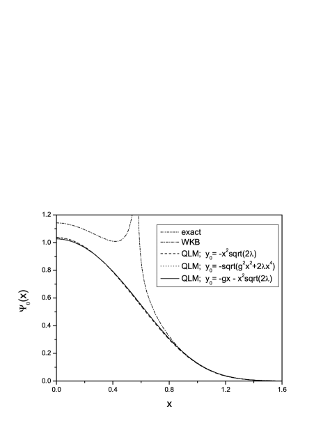
Figure 5: Comparison of the WKB, QLM and exact wave functions for the ground state of the quartic oscillator for $g=1,\lambda=10$.

Figure 6: Logarithm of the differences of the WKB and QLM wave functions with exact wave function for the ground state of the quartic oscillator for $g=1,\lambda=10.$

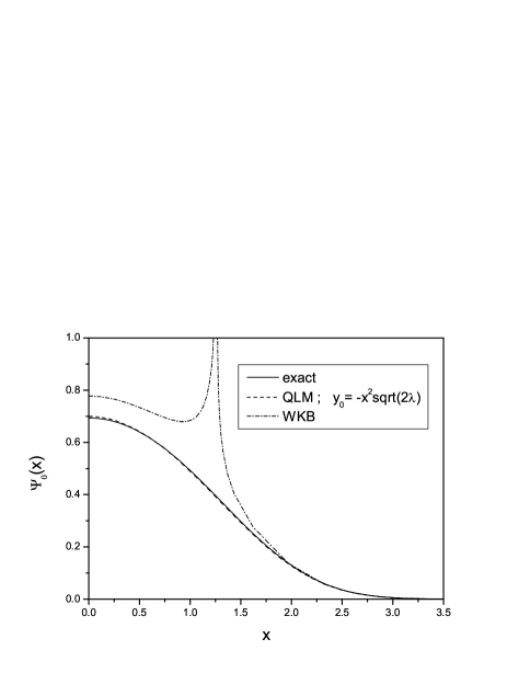
Figure 7: Comparison of the WKB, QLM and exact wave functions for the ground state of the pure quartic oscillator for $g=0,\lambda=0.1$.

Figure 8: Logarithm of the differences of the WKB and QLM wave functions with exact wave function for the ground state of the pure quartic oscillator for $g=0,\lambda=0.1.$

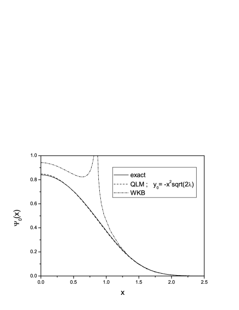
Figure 9: Comparison of the WKB, QLM and exact wave functions for the ground state of the pure quartic oscillator for $g=0,\lambda=1$.

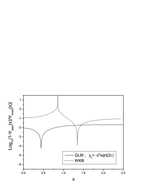
Figure 10: Logarithm of the differences of the WKB and QLM wave functions with exact wave function for the ground state of the pure quartic oscillator for $g=0,\lambda=1.$

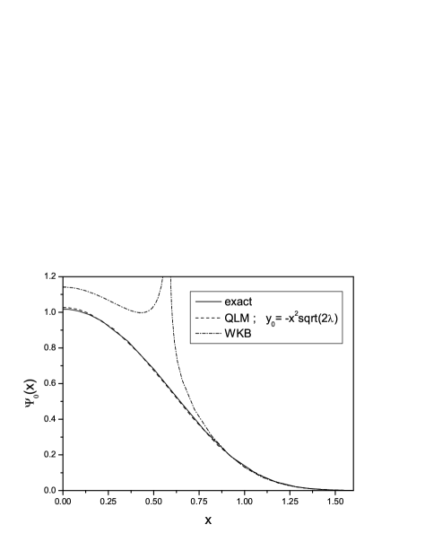
Figure 11: Comparison of the WKB, QLM and exact wave functions for the ground state of the pure quartic oscillator for $g=0,\lambda=10$.

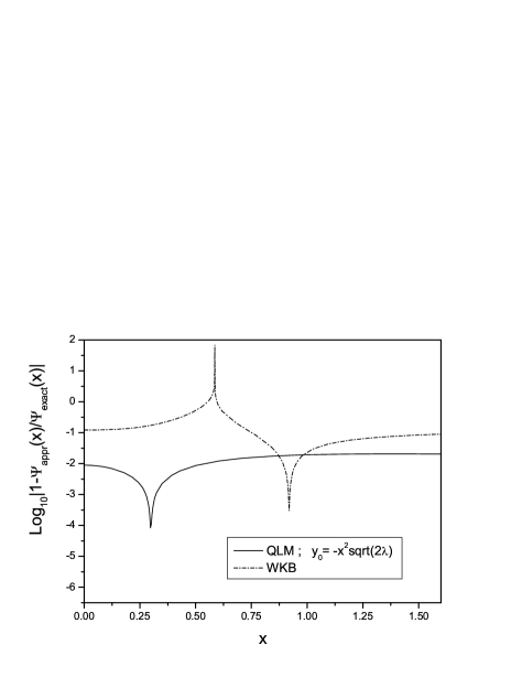
Figure 12: Logarithm of the differences of the WKB and QLM wave functions with exact wave function for the ground state of the pure quartic oscillator for $g=0,\lambda=10.$

The graphs of the wave functions for the quartic oscillator with $g=1$ and for different $\lambda$ together with the correspondent exact and WKB wave functions, are presented in Figs. 1, 3 and 5, while Figs. 2, 4 and 6 display the logarithm of the absolute value of the differences between the WKB or QLM wave functions and the exact solution for $\lambda$ being equal to 0.1, 1 and 10, respectively. The same graphs for the pure quartic oscillator ($g=0$) are presented in Figs. 7, 9, 11 and in Figs. 8, 10, 12, respectively. One can see that in all the graphs the differences between the exact and QLM solutions are two to three orders of magnitude smaller than the differences between the exact and the WKB solutions and that the QLM wave functions expressed analytically by Eqs.(11),(13) have an accuracy of between 0.1 and 1 percent. The order of magnitude better accuracy of the wave function compared to the poorer accuracy of the energies is explained by the fact that the general theorems K ; BK ; VBM1 ; MT ; VBM2 ; VBM3 for the QLM iterates show that the solutions converge quadratically with each iteration, while no such convergence theorem has been proven for the energy iterates. Note, that the dips in the Figures are artifacts of the logarithmic scale, since the logarithm of the absolute value of the difference of two solutions goes to $-\infty$ at points where the difference changes sign. The overall accuracy of the solution can therefore be inferred only at $x$ values not too close to the dips.

IV Conclusion

We calculated analytically the ground state energy and wave function of the quartic and pure quartic oscillators by casting the Schrödinger equation into the nonlinear Riccati form , which is then solved in the first iteration of the quasilinearization method (QLM), which approaches the solution of the nonlinear differential equation by approximating nonlinear terms with a sequence of linear ones and does not rely on the existence of a smallness parameter. Comparison of our results with exact numerical solutions and the WKB solutions shows that the explicit analytic expressions we obtain (12) and (14) for the ground state energy have a precision of only a few percent while the analytically expressed wave functions (11) and (13) have an accuracy of between 0.1 and 1 percent and are more accurate by two to three orders of magnitude than those given in the WKB approximation. The QLM wave function in addition possess no unphysical turning point singularities which allows one to use these wave functions to make analytical estimates of the effects of variation of the oscillator parameters on the properties of systems described by quartic and pure quartic oscillators.

The next QLM iterations could be evaluated numerically KM2 ; KMT ; KMT1 ; KM3 ; KM4 . These further QLM iterates for the different anharmonic and other physical potentials with both strong and weak couplings also display very fast quadratic convergence so that the accuracy of energies and wave functions obtained after a few iterations is extremely high, reaching 20 significant figures for the energy of the sixth iterate even in the case of very large coupling constants.

Extension of this approach to excited states and to other potentials is underway.

- (1) J. Laane, Annu. Rev. Phys. Chem. 45, 179 (1994); J. Int. Rev. Phys. Chem. 18, 301 (1999).; J. Phys. Chem. A104, 7715 (2000).
- (2) J. Zamastil, J. Cizek and L. Skala, Phys. Rev. Lett. 84, 5683 (2000).
- (3) A. S. de Castro and D. A. de Souza, Phys. Lett. A269,281 (2000).
- (4) M. Mueller and W. D. Heiss, J. Phys. A: Math. Gen 33, 93 (2000).
- (5) G. Alvarez and C. Casares, J. Phys. A: Math. Gen 33, 2499 (2000); 33, 5171 (2000).
- (6) A. Pathak, J. Phys. A: Math. Gen 33, 5607 (2000).
- (7) M. S. Child , S. H. Dong and X. G. Wang, J. Phys. A: Math. Gen 33, 5653 (2000).
- (8) G. F. Chen, J. Phys. A: Math. Gen. 34, 757 (2001).
- (9) D. Zapalla, Phys. Lett. A290, 35 (2001).
- (10) S. Giller and P. Milczarski, J. Math. Phys. 42, 608 (2001).
- (11) M. Jafarpour and D. Afshar, J. Phys. A: Math. Gen. 35, 87 (2002).
- (12) G. Alvarez, C. J. Holes and H. J. Silverstone, J. Phys. A: Math. Gen. 35, 4003 (2002); 35, 4017 (2002).
- (13) P. Amore, A. Aranda and A. de Pace, J. Phys. A: Math. Gen. 37,3515(2004).
- (14) S. Dusuel and G. S. Uhrig, J. Phys. A: Math. Gen. 37, 9275 (2004).
- (15) C. M. Bender and T. T. Wu, Phys. Rev. 184, 1231 (1969); Phys. Rev. Lett. 27 461 (1971); Phys. Rev. D 7, 1620 (1973).
- (16) B. Simon and A. Dicke, Ann. Phys. 58, 76 (1970).
- (17) R. Krivec and V. B. Mandelzweig, Computer Physics Comm. 152, 165 (2003).
- (18) R. Krivec, V. B. Mandelzweig and F. Tabakin, Few-Body Systems 34, 57 (2004).
- (19) R. Kalaba, J. Math. Mech. 8, 519 (1959).
- (20) R. E. Bellman and R. E. Kalaba, Quasilinearization and Nonlinear Boundary-Value Problems, Elsevier Publishing Company, New York, 1975.
- (21) V. B. Mandelzweig, J. Math. Phys. 40, 6266 (1999).
- (22) V. B. Mandelzweig and F. Tabakin, Computer Physics Comm. 141, 268 (2001).
- (23) V. B. Mandelzweig, Few-Body Systems Suppl. 14, 185 (2003).
- (24) V. B. Mandelzweig, Physics of Atomic Nuclei 68, 1227-1258 (2005); Yadernaya Fizika 68, 1277-1308 (2005).
- (25) R. Krivec, V. B. Mandelzweig and F. Tabakin, ”Quasilinear and WKB solutions in Quantum Mechanics”, 2006, accepted for publication
- (26) R. Krivec and V. B. Mandelzweig, Phys. Lett. A337, 354-359 (2005).
- (27) R. Krivec and V. B. Mandelzweig, Computer Physics Comm. 174, 119 (2006).
- (28) W. Janke and H. Kleinert, Phys. Rev. Let. 75, 2787 (1995).
- (29) P. M. Mathews, M. Seetharaman, S. Raghavan and V. T. A. Bhargava, Phys. Lett. A 83, 118 (1983).
- (30) R. Friedberg, T. D. Lee, Ann. Phys. 308, 263 (2003).
- (31) I.S. Gradsteyn and I.M. Ryzhik, Table of Integrals, Series and Products (Academic, New York 1994).