Multiplicative noise in the longitudinal mode dynamics of a bulk semiconductor laser

Abstract

We analyze theoretically and experimentally the influence of current noise on the longitudinal mode hopping dynamics of a bulk semiconductor laser. It is shown that the mean residence times on each mode have different sensitivity to external noise added to the bias current. In particular, an increase of the noise level enhances the residence time on the longitudinal mode that dominates at low current, evidencing the multiplicative nature of the stochastic process. A two-mode rate equation model for semiconductor laser is able to reproduce the experimental findings. Under a suitable separation of the involved time scales, the model can be reduced to a 1D bistable potential system with a multiplicative stochastic term related to the current noise strength. The reduced model clarifies the influence of the different noise sources on the hopping dynamics.

I Introduction

Fluctuations and noise are inherent to the behavior of any physical system. Their ubiquity and impact on technological applications have stimulated since long ago the study of their effects in different branches of science (statistical physics, mathematics) and technology (communications engineering).

Noise is usually perceived as a source of degradation of the properties of any system, leading to relatively small stochastic variations of a given magnitude around its deterministic (noise free) value. Such a point of view is rooted on the study of systems close to equilibrium, whose dynamics can be linearized around the deterministic steady state. However, it does not hold in systems far from equilibrium, where nonlinear corrections to the dynamics must be taken into account. In these systems, noise may not only be the responsible for the observed behavior, but it may also make possible new states and behaviors that do not exist in the noise-free limit toral . Examples of such behaviors are, for instance, the enhancement of the decay time of a metastable state (noise enhanced stability) Graham ; Mantegna , the synchronization with a weak periodic input signal (stochastic resonance) sto_res or the appearance of a periodic output (coherence resonance) coh_res . In systems with spatial degrees of freedom, noise may lead for instance to the formation of convective structures (noise-sustained structures) maxi .

The effects of noise depend on whether it is additive or multiplicative. Additive noise is present in all real, non isolated systems where the environment acts as a thermal bath. Moreover, even in an isolated system all interaction processes exhibit some degree of stochastic fluctuations that lead to internal noise in the system. This effect may be further enhanced by adding noise to the control parameters of the system. In general, the fluctuation-dissipation theorem implies that noise in a nonlinear system may have both an additive and a multiplicative component. The effects of both kinds of noise in nonlinear systems have been thoroughly studied from the theoretical point of view toral , although experimental studies of the effects of multiplicative noise are more scarce. In particular, it has been shown that the characteristic signatures of either type of noise can be profoundly modified by the presence of even a weak component of the other kind Schenzle ; Mannella . Moreover it was also found that multiplicative (parametric) noise induces a shift in the critical mean value of the parameter that controls an instability Lefever ; Moss ; Fronzoni .

In this paper we analyze theoretically and experimentally the influence of multiplicative noise on the mode hopping dynamics of a bistable semiconductor laser. Since the pumping current enters into the laser field equations in a nonlinear way, adding current noise may lead to multiplicative effects. We find that the residence times of each mode are strongly affected, and that increasing the noise added to the current is equivalent —from the point of view of residence times— to a lowering of the bias current. A theoretical model for the system under study is presented and analyzed, with the aim of understanding the observable consequences of the imposed fluctuations and the role of laser parameters. A better insight is obtained by simplification of this model to a bistable potential system. This allows us to discuss in detail the effects of current noise on the mode hopping dynamics. The results are in good agreement with the experimental observations carried out for a bulk edge-emitting semiconductor laser.

The outline of the paper is the following. In Sec. II we introduce the rate equations for a two-mode semiconductor laser and we derive from them a reduced 1D Langevin model that describes the hopping dynamics of the freely operating laser. In Sec. III we discuss in detail the reduced model and, in particular, the effect of external fluctuations of the injection current. The limit case of a slowly fluctuating current is analyzed as well and the results are compared with simulation of the rate equations. Sec. IV is devoted to the presentation of the experimental results. We draw our conclusions in Sec. V.

II Theoretical analysis

II.1 Rate equations

Our starting point is a stochastic rate-equation model for a semiconductor laser that may operate in two modes. Both modes interact with a single carrier density that provides the necessary gain. The two modes have very similar linear gains, provided that their wavelengths are almost equal and they are close to the gain peak. If $E_{\pm}$ denote the complex modal amplitudes, $N$ the carrier density and $J(t)$ the injection current, the model can be written as

$$\dot{E}_{+} =\frac{1}{2}\left[(1+i\alpha)g_{+}-1\right]E_{+}+\sqrt{2D_{sp}N}\,\xi_{+}$$ (1)

$$\dot{E}_{-} =\frac{1}{2}\left[(1+i\alpha)g_{-}-1\right]E_{-}+\sqrt{2D_{sp}N}\,\xi_{-}$$ (2)

$$\dot{N} =\gamma[J(t)-N-g_{+}|E_{+}|^{2}-g_{-}|E_{-}|^{2}]$$ (3)

where $\alpha$ is the linewidth enhancement factor petermann . The modal gains read

$$g_{\pm}\;=\;{N\pm\varepsilon(N-N_{c})\over 1+s|E_{\pm}|^{2}+c|E_{\mp}|^{2}}\;,$$ (4)

where $\varepsilon$ determines the difference in differential gain among the two modes while $N_{c}$ defines the carrier density where the unsaturated modal gains are equal. The parameters $s$ and $c$ are respectively the self- and cross-saturation coefficients. The $\xi_{\pm}$ are two independent, complex white noise processes with zero mean ($\langle\xi_{\pm}(t)\rangle=0$) and unit variance ($\langle\xi_{i}(t)\xi_{j}^{*}(t^{\prime})\rangle=\delta_{ij}\delta(t-t^{\prime})$) that model spontaneous emission. Eqs. (1-3) have to be interpreted in Itô sense Agrawal , thus the average power spontaneously emitted in each mode at any time is given by $4D_{sp}N$.

The deterministic version of Eqs. (1-3) admits four different steady state solutions: the trivial solution $E_{\pm}=0$, two single-mode solutions — $E_{+}\neq 0,\ E_{-}=0$ and viceversa — and a solution where both modes are lasing, $E_{\pm}\neq 0$. The single-mode solution where only $E_{+}$ ($E_{-}$) is lasing lacks physical sense for bias currents below $J_{+}$ ($J_{-}$) given by

$$J_{\pm}={1\pm\varepsilon N_{c}\over 1\pm\varepsilon}\;.$$ (5)

The trivial solution $E_{\pm}=0$ is the only stable solution for bias currents $J<min(J_{+},J_{-})$; for definiteness, we consider $N_{c}>1$, hence $J_{-}<1<J_{+}$. Upon increasing $J$, the trivial solution looses stability and the system switches to the solution $E_{-}\neq 0,\ E_{+}=0$ at the laser threshold, $J=J_{-}$. Further increasing the current, the sequence of bifurcations depends quite strongly on the parameters $s$, $c$ and $N_{c}$. For $c>s$, this solution may coexist with the solution $E_{+}\neq 0,\ E_{-}=0$ or even with the solution $E_{-}\neq 0,\ E_{+}\neq 0$ (in this case, only for a small current range). Finally, the solution $E_{+}\neq 0,\ E_{-}=0$ prevails.

II.2 Reduction to an effective model

In order to better assess the effects of current noise on the modal dynamics, we next reduce the rate-equation description to a bistable 1D system. In the first place, we introduce the amplitude-phase coordinates for each mode,

$$E_{\pm}\;=\;\rho_{\pm}\exp i\psi_{\pm}.$$ (6)

Using this standard transformations (see gard ) we obtain

$$\dot{\rho}_{\pm} = \frac{1}{2}\Big{[}g_{\pm}-1+\frac{2D_{sp}N}{\rho_{\pm}^{2}}\Big{]}\rho_{\pm}+\sqrt{2D_{sp}N}\,\xi_{\rho}^{\pm}$$

$$\dot{\psi}_{\pm} = \frac{\alpha}{2}g_{\pm}+\sqrt{2D_{sp}N}\,\xi_{\psi}^{\pm}$$ (7)

$$\dot{N} = \gamma[J(t)-N-g_{+}\rho_{+}^{2}-g_{-}\rho_{-}^{2}]\;.$$

Since the modal phases do not influence the evolution of the modal amplitudes and carrier density, we can disregard them without loss of generality. It is convenient to perform a further change to “cylindrical” coordinates,

$$\rho_{+}=r\cos\phi,\qquad\rho_{-}=r\sin\phi\;.$$ (8)

In these new variables, $r^{2}$ is the total power emitted by the laser, and $\phi$ determines how this power is partitioned among the two modes: $\phi=0$ ($\phi=\pi/2$) corresponds to emission in mode + (-) only, and intermediate values give different power to each mode.

Using again Ref. gard , we obtain

$$\dot{r} = \frac{r}{2}\left[\frac{N\left(1+\sigma r^{2}+\delta r^{2}\cos^{2}2\phi\right)+\varepsilon\left(N-N_{c}\right)\left(1+\sigma r^{2}+\delta r^{2}\right)\cos 2\phi}{\left(1+\sigma r^{2}\right)^{2}-\left(\delta r^{2}\cos 2\phi\right)^{2}}-1+\frac{6D_{sp}N}{r^{2}}\right]+\sqrt{2D_{sp}N}\xi_{r}\;,$$ (9)

$$\dot{\phi} = -\frac{\sin 2\phi}{2}\frac{N\delta r^{2}\cos 2\phi+\varepsilon\left(N-N_{c}\right)\left(1+\sigma r^{2}\right)}{\left(1+\sigma r^{2}\right)^{2}-\left(\delta r^{2}\cos 2\phi\right)^{2}}+\frac{2D_{sp}N}{r^{2}\tan 2\phi}+\sqrt{\frac{2D_{sp}N}{r^{2}}}\xi_{\phi}\;,$$ (10)

$$\dot{N} = \gamma\left[J-N-r^{2}\frac{N\left(1+\sigma r^{2}+\delta r^{2}\cos^{2}2\phi\right)+\varepsilon\left(N-N_{c}\right)\left(1+\sigma r^{2}+\delta r^{2}\right)\cos 2\phi}{\left(1+\sigma r^{2}\right)^{2}-\left(\delta r^{2}\cos 2\phi\right)^{2}}\right]\;.$$ (11)

where we have defined

$$\sigma={c+s\over 2},\quad\delta={c-s\over 2}.$$ (12)

The parameter $\sigma$ thus represents the gain saturation induced by the total power in the laser, while $\delta$ —given by the difference between the coefficients of cross- and self-saturation— describes the reduction in gain saturation due to partitioning of the power among the two modes. We also wish to remark that, although we worked in the Itô formalism, this form of the equations would be the same also in the Stratonovich representations gard .

The general expression just obtained for the dynamics is too involved to allow for a detailed analysis of the effects of noise. In order to simplify the theoretical analysis of this dynamical system, we further assume that: (i) The asymmetry of the modal gains is very small, i. e., $N_{c}\gtrsim 1$, $\varepsilon\ll 1$, $\delta\ll 1$; (ii) the laser operates close to threshold, so that the saturation term is small, $\sigma r^{2}\ll 1$. In this limit, we find that, to lowest order in the small terms, the dynamics is governed by

$$\dot{r} = \frac{r}{2}\left(N-1-N\sigma r^{2}+\frac{6D_{sp}N}{r^{2}}\right)+\sqrt{2D_{sp}N}\xi_{r}\;,$$ (13)

$$\dot{\phi} = -\frac{\sin 2\phi}{2}\left[N\delta r^{2}\cos 2\phi+\varepsilon\left(N-N_{c}\right)\right]+\frac{2D_{sp}N}{r^{2}\tan 2\phi}+\sqrt{\frac{2D_{sp}N}{r^{2}}}\xi_{\phi}\;,$$ (14)

$$\dot{N} = \gamma\left(J-N-r^{2}N\right)\;,$$ (15)

so the dynamics of the total intensity $r^{2}$ and of the carrier density $N$ decouple from those of the relative phase $\phi$. Thus $\phi$ is driven by the other two variables.

Moreover, the time-scale for the evolution of the relative phase $\phi$ is of second order in the small quantities, while that of $r$ and $N$ is of the first order. Since we are mainly interested in time scales long enough for the relaxation oscillations of the total power and carrier density to be totally damped, and not in the transient dynamics, we can consider that $r$ and $N$ have reached the vicinity of their steady state. By neglecting the spontaneous emission term in (13), we have that

$$r\simeq r_{0}=\sqrt{J-1\over 1+\sigma J};\quad N\simeq N_{0}={1+\sigma J\over 1+\sigma}\;.$$ (16)

A more accurate approximation would be to solve the Langevin equations for $r$ and $N$ and to insert the solution into the equation for $\phi$ in order to describe how the fluctuations of the former affect the dynamics of the latter. For simplicity, we disregard this issue under the assumption that the noise in (13) and (15) is so weak that they simply ”follow” $J$ as prescribed by (16). For a time-dependent current this approximation is valid only if $J$ does not change too fast. For example, in the case of an Orstein–Uhlenbeck process that will be considered below one must require the corresponding correlation time $\tau$ to be longer than the typical relaxation time of the total intensity. We shall see that this condition is generally met in our experimental setups.

In this representation the dynamics can be geometrically visualized as follows. The motion is constrained along a manifold (approximated as portion of a circle of radius $r_{0}$) connecting the fixed points. Radial fluctuations (i.e. fluctuations in the total intensity output) are completely neglected. The hopping dynamics is thus effectively one-dimensional and described by the ”phase” variable $\phi$, which determines how the total power is partitioned among the modes.

Altogether, the above calculation yields the reduced model

$$\dot{\phi}\;=\;-\frac{1}{2}\Big{[}a\cos 2\phi+b\Big{]}\sin 2\phi\,+\,{2D_{\phi}\over\tan 2\phi}+\sqrt{2D_{\phi}}\,\xi_{\phi}$$ (17)

where we have defined the parameters

$$a\;=\; N_{0}\delta\,r_{0}^{2}\;=\;{\delta\over 1+\sigma}\,(J-1)$$ (18)

$$b\;=\; \varepsilon(N_{0}-N_{c})\;=\;{\varepsilon\sigma\over 1+\sigma}\,(J-J_{s})\quad$$ (19)

$$D_{\phi}\;=\; {D_{sp}N_{0}\over r_{0}^{2}}\;=\;\frac{(1+\sigma J)^{2}}{(1+\sigma)(J-1)}\,D_{sp}$$ (20)

and, for later convenience, we have introduced

$$J_{s}\;=\;{(1+\sigma)N_{c}-1\over\sigma}\quad.$$ (21)

Notice that the strength of fluctuations $D_{\phi}$ depends on the current. At this stage, one may get rid of one of the three parameters. For example, one may rescale time $t\to t/a;\xi_{\phi}\to\sqrt{a}\xi_{\phi}$ so that the only independent parameters are $b/a$ and $D_{\phi}/a$. However, since we wish to understand the role of the phenomenological parameters in relation with the physical quantities we stick to the form (17). This choice is especially useful when current fluctuations will be taken into account.

To conclude this Section, we point out that the same equation (17) has been derived by Willemsen et al. will ; will2 to describe polarization switches in Vertical Cavity Surface-Emitting Lasers (VCSELs). The starting point of their derivation is the San Miguel-Feng-Moloney model Feng . We point out that the physical meaning of the variable $\phi$ is different from here as it represents the polarization angle of emitted light. Thus the potential minima correspond to the two orthogonal linearly–polarized directions. Also, Nagler et al. belgi ; belgi2 have derived a one-dimensional Langevin equation for the mode intensity in VCSEL starting from a rate equation model for the field intensities in the two polarization directions. Indeed, it can be shown that, upon the change of variable $\sin\phi=p$ and redefinition of parameters, model (17) transforms into eq. (19) and (23) of Ref. belgi . This suggests that, upon a suitable reinterpretation of variables and parameters, many of the results presented henceforth may apply also to the dynamics of VCSELs.

III Analysis of the reduced model

In this Section we analyze some features of the model in the case in which $J$ is a constant. In this case, (17) is a one-dimensional Langevin equation with additive noise originating from spontaneous emission. The force in Eq. (17) can be derived from the potential

$$U(\phi,D_{\phi})\;=\;-{a\over 16}\cos 4\phi-{b\over 4}\cos 2\phi-D_{\phi}\ln\sin 2\phi$$ (22)

The stationary distribution is thus straightforwardly computed as

$$P(\phi)\;=\;P_{0}\,\exp\left(-U(\phi,D_{\phi})/D_{\phi}\right),$$ (23)

with $P_{0}$ being the normalization constant. Notice that the potential depends explicitly on $D_{\phi}$ (i.e. on $D_{sp}$) through the repulsive logarithmic term in (22). This term is usually very small for weak noise except at the extrema $\phi=0,\pi/2$ where it diverges logarithmically. As a consequence, $P$ vanishes linearly there. Physically, this corresponds to the fact that, due to spontaneous emission, the modes are never completely switched off.

III.1 Bistability and effect of the injection current

The most important property that can be immediately drawn from the form of $U$ is that there exists a range of current values $J_{3}<J<J_{4}$ for which the system is bistable. Within this region, the system has three stationary solutions, $\phi_{\pm}$ (stable) and $\phi_{0}$ (unstable). To compute them, let us neglect the term proportional to $D_{\phi}$ in the definition of $U$: $\phi_{0}\simeq(1/2){\rm acos}(-b/a)$, $\phi_{-}\simeq 0$, $\phi_{+}\simeq\pi/2$. The bistability domain is evaluated by the condition $|b|\leq a$ yielding the approximate expressions

$$J_{3}\;=\;{\varepsilon\sigma J_{s}+\delta\over\varepsilon\sigma+\delta},\qquad J_{4}\;=\;\begin{cases}{\textstyle\varepsilon\sigma J_{s}-\delta\over\textstyle\varepsilon\sigma-\delta}&\text{if $\varepsilon\sigma>\delta$,}\\ +\infty&\text{otherwise.}\end{cases}$$ (24)

Those last expressions have been checked to be a good approximation of the exact values computed from bifurcation analysis of the deterministic rate equations in the limit of small $\varepsilon$ and $\delta$. The effect of the term proportional to $D_{\phi}$ in (22) is to make the bistability domain dependent on the noise intensity, i.e. $J_{3}(D_{\phi})<J<J_{4}(D_{\phi})$. By computing numerically the stationary points of $U(\phi,D_{\phi})$ we have found that the width of this interval of current values is reduced upon increasing $D_{\phi}$ with respect to the deterministic case. The current value $J$ controls the symmetry of the potential through the term proportional to $b$. Within the bistable region, at the critical value $J_{s}$, $b$ vanishes and the effective potential is symmetric under the transformation $\phi\to\pi/2-\phi$. In this situation the hopping between the two modes occurs at the same rate. For weak noise, $D_{\phi}\ll a$, we can easily estimate the two potential barriers as

$$\Delta U_{\pm}\;=\;\frac{(a\pm b)^{2}}{8a}\quad.$$ (25)

In the neighbourhood of the $J\simeq J_{s}$, i.e. for $(J-J_{s})\ll(J_{s}-1)$:

$$\Delta U_{\pm}\;\simeq\;\frac{\delta}{8(1+\sigma)}(J_{s}-1)\,+\,\frac{\delta\pm 2\varepsilon\sigma}{8(1+\sigma)}(J-J_{s})\;.$$ (26)

Actually, also the noise strength depends on $J$: expanding to second order around $J_{s}$ the definition of $D_{\phi}$, Eq. (20), we get

$$D_{\phi} \;\simeq\;D_{\phi}(J_{s})\Big{[}1-{\sigma(J_{s}-2)-1\over(1+\sigma J_{s})(J_{s}-1)}(J-J_{s})+$$ (27)

$${(1+\sigma)^{2}\over(1+\sigma J_{s})^{2}(J_{s}-1)^{2}}(J-J_{s})^{2}\Big{]}$$

However, it turns out that this correction to the noise is pretty small for the parameters we choose. More precisely, one can estimate that, for a given change of $J$, the relative change of $\Delta U_{\pm}$ is roughly a factor 10 larger than the one of $D_{\phi}$ note . We thus neglect the correction terms in (27) and let $D_{\phi}=D_{\phi}(J_{s})$.

In other words, we assume that changing $J$ only affects the barriers through formula (26). With this simplification the corresponding residence times are given by rmp

$$T_{\pm} \;=\; \sqrt{8\pi D_{\phi}\over a^{3}}\,\exp\Big{(}\Delta U_{\pm}/D_{\phi}\Big{)},$$ (28)

$$\;\equiv\; T_{s}\exp\Big{[}\frac{\delta\pm 2\varepsilon\sigma}{8(1+\sigma)}\,\frac{J-J_{s}}{D_{\phi}}\Big{]}$$

Here $T_{s}$ is the residence time at the symmetry point. Notice that the prefactor depends on the noise strength to leading order. Formula (28) enlightens the role of the asymmetry parameters in determining the residence times. Indeed, it predicts that the residence times should depend exponentially on the injection current with different rates. In particular, we see that increasing $J$ around $J_{s}$ may lead to an increase of both $T_{\pm}$ if $2\varepsilon\sigma<\delta$ or to an increase of $T_{+}$ accompained by a decrease of $T_{-}$ if instead $2\varepsilon\sigma>\delta$. To discriminate which of the two cases is of relevance one must thus know the values of the parameters for the laser at hand. This can only be accomplished by comparing with experimental data. For the laser at hand (see below), the measurements indicate that the case of interest is $2\varepsilon\sigma>\delta$.

III.2 Comparison with the simulation of the rate equations

Before proceeding further, we check the accuracy of the reduction by comparing with simulations of the rate equations. For defineteness, we let $\varepsilon=0.1$, $s=1.0$, $N_{c}=1.1$, $\gamma=0.01$ and $c=1.1$ and perform different runs for different values of $D_{sp}$ and for $J$ some 10% above threshold. With the above choice, $\delta=0.05$ and $\sigma=1.05$, meaning that the timescale for the slow variable $\phi$ is estimated to be about one order of magnitude larger than those of the fast ones. We also set $\alpha=0$ since, as explained above, we expect that the phase dynamics should not matter. The largest part of the simulations were performed with Euler method with time steps 0.01-0.02. For comparison, some checks with Heun method toral have also been carried on. Within the statistical accuracy, the results are found to be insensitive the the choice of the algorithm.

We first evaluated the stationary distribution $P(\phi)$ as evaluated from the data through the relation $\phi={\rm atan}(|E_{+}|/|E_{-}|)$. In Fig. 1 we compare the expression of $U$ with $-\ln P$. The simulation data reported there correspond to the current value $J=1.197$ which we empirically found to yield an almost symmetric shape of $P$. This value only differs by 2% from the one estimated from formula (21) yielding $J_{s}=1.19523...$. We also compared the numerically measured residence times $T_{\pm}$ with the prediction of the reduced model (see again Fig. 1). Since we work with values of the noise that are not extremely small, we employed the quadrature formula rmp

$$T_{\pm}\;=\;\pm\frac{1}{D}_{\phi}\int_{\phi_{-}}^{\phi_{+}}P^{-1}(x)\int_{\phi_{\pm}}^{x}\,P(y)\,dxdy\quad.$$ (29)

This functional form accurately follows the numerical data (within then 10% or so). In the inset of Fig. 1 we show that the cumulative distribution of residence times which is Poissonian as expected from the reduced model. Another series of simulations (not reported) for an asymmetric case, $J=1.18$ yield comparable results.

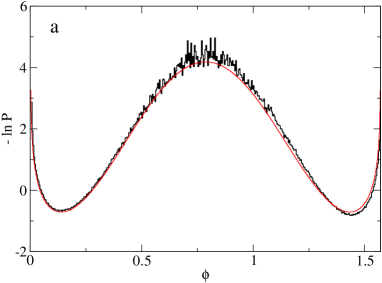
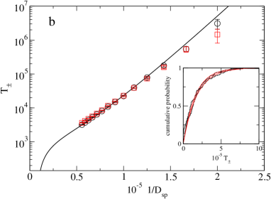
Figure 1: (Color online) Comparison between the reduced model and the simulation of the rate equations for $J=1.197$, $D_{sp}=7\times 10^{-6}$ (the other parameter values are given in the text). (a) $-\ln P$ evaluated from simulation compared with the analytical result; (b) Average residence times as a function of $1/D_{sp}$. The line is obtained from the quadrature formula (29). Inset: Cumulative distributions of residence times for $D_{sp}=7\times 10^{-6}$. The lines are the expected Poisson distribution with the same average.

III.3 Including current fluctuations

We include the fluctuation of the injected current by letting $J\longrightarrow J+\delta J(t)$. The following considerations holds for an arbitrary time dependencence of $\delta J$ under the limitations necessary to eliminate Eq. (13). For defineteness, we may focus on the case in which $\delta J$ is a Ornstein-Uhlenbeck process with zero average $\langle\delta J(t)\rangle\;=\;0$ and correlation time $\tau$:

$$\dot{\delta J}\;=\;-{\delta J\over\tau}+\sqrt{2D_{J}\over\tau}\,\xi_{J}$$ (30)

that means

$$\langle\delta J(t)\delta J(0)\rangle\;=\;{D_{J}}\exp(-|t|/\tau)\quad.$$ (31)

This choice is suitable to model the finite-bandwith of the noise generator employed in the experimental setup. Notice that $\tau$ and the variance of fluctuations ${D_{J}}=\langle\delta J^{2}\rangle$ can be fixed independentely.

The effect of a time-dependent current is twofold. First, the potential becomes fluctuating: the $a$, $b$ and $D_{\phi}$ coefficients become time-dependent quantities and the potential barriers $\Delta U_{\pm}(t)$ change accordingly. For weak noise, and close to the symmetry point $\delta J\ll(J_{s}-1)$ they are computed from approximated formula (26) with $J-J_{s}$ replaced by $\delta J(t)$,

$$\Delta U_{\pm}(t)\;\simeq\;\frac{\delta}{8(1+\sigma)}(J_{s}-1)\,+\,\frac{\delta\pm 2\varepsilon\sigma}{8(1+\sigma)}\delta J(t)\,.$$ (32)

The barriers’ height depends linearly on $\delta J$ to leading order. Obviously, this last expression makes sense only when the fluctuating term is sub-threshold i.e. whenever the system is bistable (a large enough $\delta J$ could always occur making the potential single-well). The second effect is on the additive noise strength. Since $D_{\phi}$ depends on $\delta J$ the amplitude of spontaneous emission is renormalized. Indeed, since $\xi_{\phi}$ is $\delta-$ correlated, the process $\sqrt{2D_{\phi}(J)}\,\xi_{\phi}$ can be replaced by $\sqrt{2\langle D_{\phi}\rangle}\,\xi_{\phi}$ where the average is over the fluctuations of the variable $\delta J$. Using the expansion (27) we get

$$\langle D_{\phi}\rangle\;=\;D_{\phi}(J_{s})\Big{[}1+{(1+\sigma)^{2}\over(1+\sigma J_{s})^{2}(J_{s}-1)^{2}}\,D_{J}\Big{]}$$ (33)

The coefficient in front of $D_{J}$ is strictly positive meaning that current fluctuations always enhance spontaneous ones. However, as argued in Section III.1 for the case of static changes of $J$, it turns out that the relative change $\Delta U_{\pm}$ is larger than that of $D_{\phi}$ if $D_{J}\ll(J_{s}-1)^{2}$ (see however again note note ). Therefore, in the following we can safely set $\langle D_{\phi}\rangle\;\simeq\;D_{\phi}(J_{s})$.

Although expression (32) is sufficient to draw some conclusion than can be experimentally tested, it is useful to write down also the full Langevin equation associated with the problem. Putting al the terms together we find that, to first order in $\delta J$, equation (17) transforms to

$$\dot{\phi}\;=\;-U^{\prime}(\phi,D_{\phi})-V^{\prime}(\phi,D_{\phi})\,\delta J+\sqrt{2D_{\phi}}\,\xi_{\phi}$$ (34)

where

$$-V^{\prime}(\phi,D_{\phi})\;=\;-\frac{1}{2(1+\sigma)}\Big{(}\delta\cos 2\phi+\varepsilon\sigma\Big{)}\sin 2\phi$$ (35)

(for simplicity we neglected again the dependence of $D_{\phi}$ on the current fluctuations). The multiplicative term can be thus derived from the “potential”

$$V(\phi)\;=\;-{\delta\over 16(1+\sigma)}\cos 4\phi-{\varepsilon\sigma\over 4(1+\sigma)}\cos 2\phi.$$ (36)

For an arbitrary choice of the parameters, $V$ has a different symmetry with respect to $U$ meaning that the effective amplitude of multiplicative noise is different within the two potential wells. If this difference is large enough, current fluctuation will remove the degeneracy between the two stationary solutions.

Non-Markovian equations of the form (34) have been thoroughly studied in the literature (see e.g. h94 ; h95 ; iw96 ; m96 and references therein). Although their full analytical solution for arbitrary $\tau$ is not generally feasible, several approximate results can be provided in some limits. In the following Section we will discuss the case which is of experimental importance.

III.4 The kinetic limit

Altogether, the mode switching can be seen as an activated escape over fluctuating barriers given by (32). The statistical properties of the latter process is controlled by the current fluctuations. To assess the nature of the stochastic process at hand, it is important to discuss the relevant time scales. In particular, one should compare the relaxation time $T_{R}$ within the wells with both $\tau$ and the residence times $T_{\pm}$. If $T_{R}<\tau$ we are in the colored noise case. An estimate of $T_{R}$ is the inverse of the curvature at $\phi_{0}$ that is approximatively given by $1/a$. For example, with the set parameters chosen in Sec. III.2 one finds $T_{R}\sim 200$ in model units.

In bulk semiconductor lasers the residence times are generally much larger than $T_{R}$ (the switching time between the two states). Typically, $T_{R}\sim 5-10ns$ while residence times may range between 1 and 100 $\mu s$. The noise correlation time can be somehow tuned but the noise generator limit $\tau$ to be larger of 100 $ns$ (8.8 Mhz is the maximal bandwidth used in the experiment, see Section IV below). Moreover, the frequency of the relaxation oscillations of the total power is typically above 1 GHz, and its damping occurs on a $ns$ time scale, in accordance with the assumptions made in the theoretical analysis.

At least to a first approximation, we can thus consider the limit of large $\tau$. This justifies a further reduction of the problem to a kinetic description which amounts to neglect intrawell motion and reduce to a rate model describing the statistical transitions in terms of transition rates. If we consider $\tau$ as a time scale of the external driving we can follow the terminology of Ref. talk and refer to this situation as the “semiadiabatic” limit of Eq. (34). We will now consider separately two limit cases.

III.4.1 Slow barrier, rare hops: $T_{R}\ll\tau\ll T_{\pm}$

This corresponds to the situation in which spontaneous emission noise is very weak. In this case the residence time is basically the shortest escape time, which in turn correspond to the lowest value of the barrier (the noise is approximatively constant in the current range considered henceforth). For the case of interest, $\delta<2\varepsilon\sigma$ we can use (32) to infer that the minimal values of $\Delta U_{\pm}$ should be attained for $\delta J\propto\mp\sqrt{D_{J}}$ respectively. This yields

$$T_{\pm}\;\simeq\;T_{s}\exp\Big{[}-K\frac{2\varepsilon\sigma\pm\delta}{1+\sigma}\,\frac{\sqrt{D_{J}}}{D_{\phi}}\Big{]}$$ (37)

where $K$ is a suitable numerical constant. The ratio of residence times $\eta$ is thus exponential in the noise RMS:

$$\eta\;\equiv\;{T_{+}\over T_{-}}\;=\;\exp\Big{(}-K\frac{2\delta}{1+\sigma}{\sqrt{D_{J}}\over D_{\phi}}\Big{)}$$ (38)

Notice that $\delta$ controls the asymmetry level: if $\delta\ll 2\varepsilon\sigma$ the two residence times decrease at approximatively the same rate. This prediction is verified in the simulations reported below and also in the experiment.

III.4.2 Slow barrier, frequent hops: $T_{R}\ll T_{\pm}\ll\tau$

This corresponds to the adiabatic limit in which the time scale of the external driving is slower than the intrinsic dynamics of the system talk . The results of this subsection are thus not of direct relevance for interpreting the experimental results reported here. However, we discuss also this regime for completeness and to emphasize the differences with respect to the previous case.

To a first approximation we can here treat current fluctuations in a parametric way. The switch time will be the average of escape times over the distribution of barrier fluctuations, i.e. $\langle T_{\pm}\rangle_{\delta J}$. Using again the approximation (32), since the variable $\delta J$ is Gaussian, using the identity $\langle\exp{\beta z}\rangle=\exp(\beta^{2}\langle z^{2}\rangle/2)$ one gets m96

$$T_{\pm}\;\simeq\;T_{s}\exp\Big{[}{2(\delta\pm 2\varepsilon\sigma)^{2}\over(1+\sigma)^{2}D_{\phi}^{2}}\,D_{J}\Big{]}.$$ (39)

This means that in this limit the residence times increase exponentially with the noise variance (i.e. exponentially with the square of RMS). In other words, the fluctuations always increase the effective barriers albeit asymmetrically.

III.5 Comparison with the rate equations in the presence of current noise

The above analysis shows that the effect of multiplicative noise may strongly depend on the actual parameters of the model, in particular of the ratio between $\varepsilon$ and $\delta$. Accordingly, the simmetry-breaking effects can vary considerably depending on the parameter $\delta$, see Eq. (38). To further clarify this dependence and as a check of the prediction, we performed some simulations of the rate equations (1-3) together with (30). We investigated the effect of changing the value of the cross-saturation coefficient $c$, keeping the other parameters fixed the same used in Section III.2. The DC value of the current $J$ has been again choosen empirically to yield an almost symmetric distribution $P(\phi)$ for $D_{J}=0$.

We set $\tau=4\times 10^{4}$ that correspond roughly to the experimental values. In Fig. 2 we plot $-\ln P$ for $c=1.1$ and $c=1.3$ corresponding to $\delta=0.05$ and $\delta=0.15$ respectively. In the second case the multiplicative effect of the noise is stronger and leads to a sizeable distortion of the curve while for small asymmetries the curves basically mantain their symmetry.

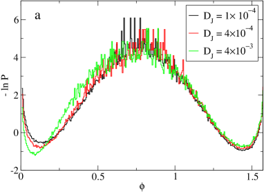
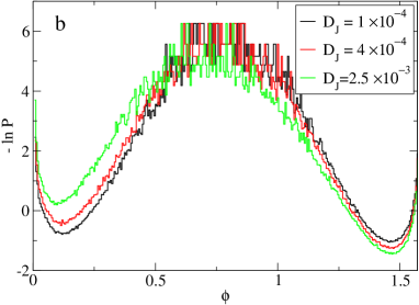
Figure 2: (Color online) Simulation of the rate equation with current fluctuations: $-\ln P$ for different amplitudes of imposed noise $D_{J}$; for $c=1.1$, $J=1.197$, $D_{sp}=7\times 10^{-6}$ (a) and $c=1.3$, $J=1.194$, $D_{sp}=1.5\times 10^{-5}$ (b).

The same type of behavior can be observed in the dependence of the residence times on the current fluctuations. Fig. 3a illustrates how for $c=1.1$ ($\delta=0.05$) the residence times decrease at approximatively the same rate upon increasing current fluctuations and the ratio $\eta$ remains very close to 1. On the contrary, upon increasing the cross-saturation coefficient to $c=1.3$ ($\delta=0.15$) a sizeable symmetry breaking (Fig. 3b): one of the two times remains almost constant while the other decreases. This is in agreement with formulae (37) and (38). Indeed, the ratio between the decay rates of $\eta$ obtained from the fits (insets of Fig. 3) is about 40, which is roughly a factor 2 of the corresponding value as computed from (38) with the simulation parameters at hand.

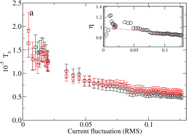
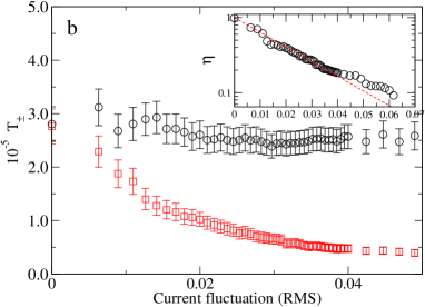
Figure 3: (Color online) Simulation of the rate equation with current fluctuations: Residence times $T_{+}$ (squares) and $T_{-}$ (circles) for $c=1.1$ (a) and $c=1.3$ (b). The parameters are the same as in Fig. 2. The insets report the ratio of the two times and the dashed line is an exponential fit, see expression (38).

IV Experimental Results

IV.1 Experimental set-up

The experimental setup is similar to the one described in IEEE ; AppB . Several edge-emitting semiconductor laser were tested: two Hitachi Hlp 1400 lasing at 840 nm and three Sharp LT021 MD lasing at 780 nm. These lasers are GaAlAs double-hetero-structure with a bulk active region and cleaved, uncoated facets. The wavelength separation between consecutive longitudinal-modes is around 0.3 nm, and the laser emission occurs in a single-transverse mode. The laser package temperature is stabilized up to $\rm 0.01^{o}C$ and the laser current is controlled with a very stable (up to $\rm 1~{}\mu A$) power supply. The laser is optically isolated from the rest of the set-up by means of an optical diode that avoid spurious back reflection. The total laser emission is detected by an Avalanche Photodiode detector (APD) (DC-1.5 GHz bandwidth) while the time-averaged optical spectrum is measured by an Agilent 86140B spectrum analyzer. Individual longitudinal mode detection is obtained by sending part of the laser output into a monochromator (resolution $0.5~{}\AA$) with two independent output slits. The monochromator can be set in order to have at the two exits two different longitudinal modes emitted by the laser. Each longitudinal mode intensity is then monitored by two APD detectors (DC-1.5 GHz bandwidth) placed beyond the slits. The outputs from these detectors are monitored on a LeCroy 7200A (500 MHz analogue bandwidth, 1 GS/s). The power spectra of the signals can be monitored using an Agilent E4403B spectrum analyzer.

IV.2 Longitudinal mode-hopping

Two control parameters can be directly varied in this system: the pumping current $J$ and the temperature of the laser substrate $T_{sub}$. As described in IEEE ; AppB , the optical spectra of the lasers tested show a single longitudinal mode emission for most of the parameter values ($J$, $T_{sub}$). However, there exist small regions in the parameter space where the lasers are bistable and exhibit mode-hopping between two longitudinal modes. A basic explanation of the destabilization of the leading longitudinal mode is that, fixing the $T_{sub}$ and increasing $J$ the wavelength of the cavity resonance increases due to Joule heating of the semiconductor medium. The gain curve peak shifts towards longer wavelength as well, but at a larger rate. Eventually, the dominating longitudinal mode looses its stability in favour of a longer wavelength one, which has become more resonant with the gain peak. The same happens when, for fixed $J$, $T_{sub}$ is increased. This type of transition among lasing modes is well-known petermann and occurs sharply in the parameter space.

Observation of this regime of stochastic mode-hopping has been reported in several papers Ohtsu ; Ohtsu2 ; IEEE . Its most relevant features are: (i) the total emitted intensity remains almost constant though each longitudinal mode is switching on and off. In other words, the anti-correlation of the two modal intensities is very strong (better than $-0.95$ in our case); (ii) the distribution of residence times in a mode, defined as the interval between a switching-on and a switching-off event, is Poissonian; (iii) a sweep of the pump current across this parameters’ region, reveals the existence of an hysteresis cycle for the modal emission which is a signature of bistability between the two longitudinal modes. It is thus clear that these features are straightforwardly explained by the theoretical analysis presented above.

The study of the fluctuations of the laser emission can be carried out by monitoring the modal intensities normalized to the total intensity output: $m_{I}=i_{I}/i_{tot}$ and $m_{II}=i_{II}/i_{tot}$. The mode labeled with $I$ is the one with larger wavelength. These are related to $\rho_{\pm}$ defined in the theoretical analysis, by $m_{I,II}=\rho_{\pm}^{2}/r_{0}^{2}$. Then, it is useful to represent the state of the system in the phase space (${m_{I}}^{1/2},{m_{II}}^{1/2}$). Hence, the variable $\phi$ used in the theory is simply the angle that this vector forms with the horizontal axis. The strong anticorrelation of the modal intensities implies that the modulus of this vector is almost constant and equal to one. In Fig. 4 we plot the the probability distribution function in the space (${m_{I}}^{1/2},{m_{II}}^{1/2}$). The maxima of the distribution correspond to the two stable modes involved in the hopping. It is evident that the relevant dynamics occur on a portion of the unit circle as assumed in the simplified theory.

The probability distribution functions of the angular variable $\phi$ as obtained from the experiment are reported in Fig. 5 for different values of the pumping current. For every $\phi$ we have included in the histograms all the points along the radial direction. Two peaks located around $\phi=0.2$ and $\phi=1.4$ are found, corresponding to the activation of the mode $I$ and $II$ respectively. In Fig. 5a we plot the distribution of $\phi$ for the case of Fig. 4, where the modal emission is symmetric, $J\simeq J_{s}$. The measurements show that upon changing the pumping current an asymmetric situation settles down, where the laser emission on one of the two modes is favored. In particular, an decrease (resp. increase) of $J$ with respect the value of Fig.  4, enhances the stability of the mode labeled by $II$ (resp. $I$), see Fig. 5b,c respectively. In all cases, the logarithm of the distribution can be fitted with the function (see Eqs. (22) and (23)) $-\frac{A}{16}\cos 4\phi-\frac{B}{4}\cos 2\phi-D\ln\sin 2\phi+C$.

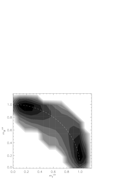
Figure 4: Experimental probability distribution of the normalized modal amplitudes (see text). The histogram is represented in logarithmic scale with a grey scale code from white (low probability) to black (high probability); $J=95.9mA$, $T_{sub}=20.4^{o}C$.

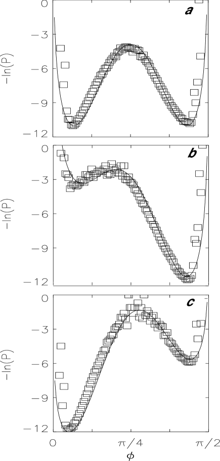
Figure 5: The logarithm of the experimental probability distribution function of the variable $\phi$ (squares) for three different values of the current, $T_{sub}=20.4^{o}C$. The line is the fitting with the function given in the text. (a) $J=95.9mA$, fitting parameters $A=108.5,B=0,D=4.6,C=-10.6$; (b) $J=95.1mA$, fitting parameters $A=85,B=-18.7,D=4.9,C=-8.1$; (c) $J=96.6mA$, fitting parameters $A=90,B=13.5,D=2.5,C=-7.2$.

The dependence of the average residence times, $T_{I}$ and $T_{II}$, on the pumping current is shown in Fig. 6. As predicted by formula (28), both times depend exponentially on $J$ and the two curves have different absolute values of the slopes (remember the remark at the end of Sec. III.1). Incidentally, this implies that the quantity $(T_{I}+T_{II})/2$ increases with the current, meaning that hops become more and more rare. Moreover, the ratio $\eta=T_{I}/T_{II}$ increases exponentially with the current as shown in the inset of Fig. 6. This behaviour is also consistent with formula (28).

Figure 6: Average residence times for mode $I$ (triangles) and $II$ (squares) as a function of pumping current, $T_{sub}$=$20.4^{o}C$. Inset: the ratio $T_{I}/T_{II}$.

IV.3 Effect of noise addition onto the pumping current

In a semiconductor laser driven by a constant ($DC$) current, the main source of noise is the spontaneous emission within the semiconductor medium. This noise source cannot be varied directly through the control parameters. Fluctuations can be added into the system externally by adding electrical noise on the pumping current. This signal employed in our setup has zero-mean, a bandwidth ranging from 100 Hz to 8.8 MHz and it is AC-coupled to the laser bias current.

In Fig. 7a we show how the average residence times $T_{I,II}$ change upon increasing the current noise level around the static value $J_{s}$. The times are affected in a strongly asymmetric way: while $T_{II}$ is almost unchanged, $T_{I}$ decreases exponentially. In Fig. 7b we plot the probability distribution function of the angular variable $\phi$ for different values of the pump noise. The experimental evidence confirms that the asymmetry of the probability distribution increases upon increasing the noise level. It is interesting to remark that an increase of noise level is equivalent, from the point of view of the residence times, to a decrease of the $DC$ pumping current. This experimental result confirms that the imposed noise does affect the dynamics in a multiplicative way. The qualitative agreement between the experimental data and the simulations reported in Figs. 2b and 3b supports the validity of our modelling. The exponential dependence of the ratio $\eta$ on the RMS of the fluctuation predicted by the analysis of the reduced model, Eq. (38), is indeed observed in the experiment (see Fig. 8). This is another indication that confirms that the kinetic description suffices to capture the mode-hopping dependence on noise level.

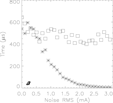
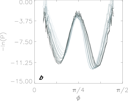
Figure 7: Effect of external noise added on the pump current. The measurements are performed on a laser sample different from the one used for Figs. 4,5, 6, requiring slightely modified values for the control parameters to obtain the same behaviors. (a) The average residence times $T_{I}$ (stars) and $T_{II}$ (squares) as a function of the RMS level of the noise added to the pumping current, $T_{sub}=20.5^{o}C$, $J$=92.0 mA. (b) The corresponding logarithm of probability distribution function of the variable $\phi$ for different levels of current noise (noise increases from dark trace to grey trace).

Figure 8: The ratio of residence times $\eta=T_{I}/T_{II}$ as a function of the RMS level of the noise added to the pumping current (parameters are the same of Fig. 7).

V Conclusions

In this paper we have explored experimentally and theoretically the effects of external current noise on the mode-hopping dynamics of a bistable semiconductor laser. We have shown that the residence times of each mode are strongly affected, bearing the typical signatures of multiplicative noise. We have investigate a theoretical model based on a rate-equation description, where the bias current enters parametrically into the evolution of the modal amplitudes, hence the multiplicative character of its fluctuations. Numerical simulations of the rate equations are in good qualitative agreement with the experimental observations. Moreover, the reduction of this model to a 1D Langevin equation describing activated escape over a fluctuating barrier has allowed us to draw some predictions (e.g. the dependence of residence times on noise strength) and to better understand the role of the physical parameters. Depending on their values, the fluctuating part of the effective potential may have a different parity with respect to the static one. This explains the observation that imposed fluctuations have different effects on the hopping rates (symmetry breaking).

The reduced model and many of the results presented here could be useful to describe also polarization switching in VCSELs driven by external noise. Indeed, experimental data show strong similarities between this phenomenon gianni3 ; gianni4 and the longitudinal mode dynamics. On the theoretical side, this analogy is supported by the fact that the polarization dynamics in VCSELs is described by models that are very similar to the one discussed here will ; will2 ; belgi . The inclusion of current noise effects along the same line above reported should be feasible once the typical time scales and parameters for such a class of lasers are evaluated. This work, that we plan to undertake in the future, will provide a common theoretical basis to the stochastic dynamics of bistable semiconductor lasers.

- (1) For a review, see for instance R. Toral and M. San Miguel, ”Stochastic effects in physical systems”, in Instabilities and Nonequilibrium Structures VI, 35-130, edited by Enrique Tirapegui, Javier Martinez, and Rolando Tiemann, Kluwer Academic Publishers (2000).
- (2) R. Graham and A. Schenzle, Phys. Rev. A 26, 1676 (1982).
- (3) R. N. Mantegna and B. Spagnolo, Phys. Rev. Lett. 76, 563 (1996).
- (4) R. Benzi, A. Sutera, and A. Vulpiani, J. Phys. A 14, 453 (1981); C. Nicolis, G. Nicolis, Tellus 33, 225 (1981).
- (5) A. Pikovsky and J. Kurths, Phys. Rev. Lett. 78, 775 (1997).
- (6) M. Santagiustina, P. Colet, M. San Miguel, and D. Walgraef, Phys. Rev. Lett. 79, 3633 (1997).
- (7) A. Schenzle and H. Brand, Phys. Rev. A 20, 1628 (1979).
- (8) R. Mannella, S. Faetti, P. Grigolini, P. V. E. McClintock and F. E. Moss, J. Phys. A 19, L699 (1986).
- (9) R. Lefever and W. Horsthemke, Bull. Math. Biol. 41, 469 (1979).
- (10) F. Moss and G. Welland, Phys. Lett. A 89, 273 (1982).
- (11) L. Fronzoni, R. Mannella, P. V. E. McClintock and F. Moss, Phys. Rev. A 36, 834 (1987).
- (12) K. Petermann, Laser Diode Modulation and Noise, ADOP-Kluwer Academic Publisher, Dordrecht (The Nederlands), 1988.
- (13) G. P. Agrawal and N. K. Dutta, Long wavelength semiconductor lasers, Van Nostran Reinhold, New York, 1986.
- (14) C. W. Gardiner, Handbook of stochastic methods (second edition), Springer-Verlag, Berlin, 1985.
- (15) M.B. Willemsen, M. U. F. Khalid, M. P. van Exter and J. P. Woerdman, Phys. Rev. Lett. 82, 4815 (1999).
- (16) M. P. Van Exter, M.B. Willemsen, J. P. Woerdman, Phys. Rev. A 58 4191 (1998).
- (17) M. San Miguel, Q. Feng, J.V. Moloney, Phys. Rev. A 52 1728 (1995)
- (18) B. Nagler et al., Phys. Rev. A 68 013813 (2003).
- (19) B. Nagler et al., Phys. Rev. E 67 056112 (2003).
- (20) P. Hänggi, P. Talkner and M. Borkovec, Rev. Mod. Phys. 62 251 (1990).
- (21) Actually this statement is not correct when . As seen from Eq. (26), in this case is hardly affected by a change in and the change of noise amplitude becomes relevant, Since the parameters are independent we restrict to the generic case in which the above condition is not fullfilled.
- (22) P. Hänggi, Chem. Phys. 180 157 (1994)
- (23) A. J. R. Madureira et al., Phys. Rev. E 51 3849 (1996).
- (24) M. Marchi et al. , Phys. Rev. E 54 3479 (1996).
- (25) J. Iwaniszewski, Phys. Rev. E 54 3173 (1996).
- (26) P. Talkner, J. Luczka, Phys. Rev. E 69 046109 (2004).
- (27) L. Furfaro, F. Pedaci, X. Hachair, M. Giudici, S. Balle, J. Tredicce, IEEE J. of Quantum Electron. 40, 1365 (2004).
- (28) F. Pedaci, M. Giudici, G. Giacomelli, J. R. Tredicce, Appl. Physics B81, 993 (2005).
- (29) M. Ohtsu, Y. Teramachi, Y. Otsuka, and A. Osaki, IEEE J. of Quantum Electron. vol. 22, 535 (1986).
- (30) M. Ohtsu and Y. Teramachi, IEEE J. Quantum Electron. vol. 25, 31 (1989).
- (31) G. Giacomelli and F. Marin, Quantum Semiclass. Opt. 10, 469 (1998).
- (32) S. Barbay, G. Giacomelli and F. Marin, Phys. Rev. E 61, 157 (2000).