Generic features of the wealth distribution in ideal-gas-like markets

Abstract

We provide an exact solution to the ideal-gas-like models studied in econophysics to understand the microscopic origin of Pareto-law. In these classes of models the key ingredient necessary for having a self-organized scale-free steady-state distribution is the trading or collision rule where agents or particles save a definite fraction of their wealth or energy and invests the rest for trading. Using a Gibbs ensemble approach we could obtain the exact distribution of wealth in this model. Moreover we show that in this model (a) good savers are always rich and (b) every agent poor or rich invests the same amount for trading. Nonlinear trading rules could alter the generic scenario observed here.

Wealth and its distribution plays an important role in society. Economic policies, natural resources, and human psychology are certainly important factors which govern the distribution of wealth. However, some features of the distribution are independent of the details. As pointed out by Pareto Pareto , a large fraction of the wealth in any economy is always owned by a small fraction of the population and vice versa. His empirical formulation, later named as Pareto’s law, describes that the distribution of wealth $w$ follows a power law $P(w)=w^{-\gamma}$. Recent studies Real of wealth distribution in several countries also confirm that it is indeed the behavior for the ”rich”, which is only about $3\%$ of the population. The rest follow a exponential or Gibbs distribution. An interesting analogy Yako00 ; Bikas03 has been drawn between the economic system and a system of ideal gas where particles and their energies are modeled as agents and their wealth. Collision between particles is similar to trading between agents where energy or wealth is neither created nor destroyed; it is just redistributed between agents. As pointed out by YakovenkoYako00 , such a process obviously generates Gibbslike distributions observed for the majority of the population.

Then what is the origin of power-law for the rich? Chakrabarti and co-workers Bikas03 ; Mann04 pointed out that saving is an important factor which decides and dictates the distribution for the rich. In a generic society agents have different opinions and concepts of saving and, accordingly, each agent saves a fraction of his wealth and invests the rest for trading. The available wealth is then shared randomly between two interacting agents. These models generically predict a power-law distribution of wealth with $\gamma=2$. Later studies indicate that $\gamma$ is not truly universal and can be changed in certain specific cases. A strikingly different distribution of wealth is observed in a system of like-minded agents (when saving propensity is the same for every agent), where it is asymmetric and peaked below the average. Numerically it could be well fitted to a Gamma distribution Patri04 ; however, recent studies indicate a discrepancy Rich04 . The exact form of the distribution is still an open question and in this paper we refer to it as $Gamma$-like distribution.

It is important to make a distinction between wealth and money, although in this paper we have used one as a synonym of the other. Wealth is usually refered to things that have economic utility, $e.g.$, money and property. During an exchange of money for tangible property, the wealth of the involved agents does not change. Again, the effective value of tangible property in terms of monetary units changes in time violating the conservation of total wealth. Such realistic features of economy are not included in Yako00 and Bikas03 ; Mann04 ; however, these simple minimal models remarkably explain the universal two-class feature of the wealth distributions. In particular, numerical studies by Chatterjee, Chakrabarti, and Manna (CCM) Mann04 clearly suggest an algebraic distribution of wealth for the rich. Later studies (mainly numerical Book and a few analytical Das03 ), also reveal that algebraic distributions are generic for the CCM model and its variants. Exact results, however, are far from reach. In this paper we will focus on the exact solution of a generic ideal-gas-like economy where saving propensities of agents are random and distributed arbitrarily. The CCM model is a special case where the distribution of saving propensity is uniform. Our results clarify why $\gamma=2$ for most cases and also show a way of getting a distributions when $\gamma\neq 2$. We have also pointed out that in these class of models (a) good savers are always rich and (b) every agent invests on the average a fixed amount for trading.

To be more precise about the model let us consider a system of $L$ agents having their saving propensity $0\leq\lambda<1$ distributed as $g(\lambda)$. The agents are labeled as $i=0,1,\dots,L-1$ such that $\lambda_{0}\leq\lambda_{1}\leq\dots\leq\lambda_{L-1}$. Let us assume that initially total wealth is randomly distributed among agents and the average is

$$\bar{E}=\frac{1}{N}\sum_{i}E_{i}.$$

A pair of agents, chosen randomly in this model, exchange their wealth in the following way. Each agent $i$ saves $\lambda_{i}$ fraction of its wealth and invests $(1-\lambda_{i})$ fraction for exchange. The available wealth for the pair $i$ and $j$ is then shared among the agents in a random fashion. Thus,

$$E_{i} \to \lambda_{i}E_{i}+\epsilon_{ij}[(1-\lambda_{i})E_{i}+(1-\lambda_{j})E_{j}],$$ (1)

$$E_{j} \to \lambda_{j}E_{j}+(1-\epsilon_{ij})[(1-\lambda_{i})E_{i}+(1-\lambda_{j})E_{j}],$$ (2)

where $0<\epsilon_{ij}<1$ is chosen randomly for each trading from a distribution $h(\epsilon)$ where the average is $r=\langle\epsilon_{ij}\rangle$.

It is quite evident that when $\lambda_{i}=0$, the model is identical to the ideal gas model, where particles encounter random elastic collisions. In this case, irrespective of the initial distribution of energy or wealth, in equilibrium (after a sufficiently large number of collisions) wealth is redistributed according to Gibbs distribution with a temperature suitably defined by $\bar{E}$. It explains the wealth distribution for a majority which follows the exponential law. To understand the origin of the power-law for the rich, as explained by the authors of Bikas03 we must introduce savings. However, note that the particles are no more identical once the saving propensity is different for different agents. Then, one’s saving propensity is his identity. It is thus appropriate to study the ensemble of such systems. The idea of an ensemble is not new in statistical physics. It is a collection of infinitely many mental copies of systems prepared under the same macroscopic conditions. Physical observables are then needed to be averaged over the ensemble to get rid of the microscopic fluctuations. Let us study an ensemble of $N$ systems labeled by $\alpha=1,\dots,N$, prepared with the same average energy $\bar{E}$. Thus, in each system $\{\lambda_{i}\}$ are the same whereas the initial wealth is different in different systems. Also different is the sequence of pairs $(i,j)$ selected for trading and the sharing of available wealth between the pair ($\epsilon_{ij}^{\alpha}$) during each trading. Thus, it is appropriate to find out the distribution of ensemble-averaged wealth defined by

$$w_{i}=\frac{1}{N}\sum_{\alpha}^{N}E_{i}^{\alpha},$$ (3)

where $E_{i}^{\alpha}$ is the wealth of an individual $i$ in system $\alpha$. In a large system ($L\to\infty$) agent $x=i/L$ has wealth $w(x)$ and saving propensity $\lambda(x)$. Since $x$ is uniform in $(0,1)$, $\lambda(x)$ can be obtained from the conservation of probability element

$$g(\lambda)d\lambda=dx.$$ (4)

Now we can proceed to derive an effective model of exchange for $w(x)$. First, note that since the pair of agents are chosen randomly for exchange, a specific agent $x$ interacts with different agents in different systems in the ensemble. Eventually agent $x$ interacts with every other agent when $N\to\infty$. Second, that for a given pair $x$ and $y$, $\epsilon_{xy}$ is different in different systems and the effective sharing is $\langle\epsilon_{xy}\rangle=r$. Thus, during trading with $y$, the average wealth $w(x)$ of agent $x$ changes to $w^{\prime}(x;y)$, where

$$w^{\prime}(x;y)=[r+\lambda(x)(1-r)]w(x)+r[1-\lambda(y)]w(y).$$ (5)

Since $w(x)$ is stationary in the steady state, we must have

$$w(x)=\int_{0}^{1}w^{\prime}(x;y)dy.$$ (6)

Equation (6), together with (5), can be solved as

$$w(x)=\frac{C}{1-\lambda(x)},$$ (7)

where $C$ is an arbitrary constant, can be fixed by the average wealth $\bar{E}$. Explicitly,

$$\int_{0}^{1}w(x)dx=\bar{E}.$$ (8)

Note that neither $r$ nor $h(\epsilon)$ appears in Eq. (7).

The distribution of $w$ must satisfy $P(w)dw=dx$; thus

$$P(w)=\frac{dx}{dw}=\frac{Cg(1-C/w)}{w^{2}}.$$ (9)

Here the quantity after the last equality is derived using Eqs. (7) and (4). It is clear from (9) that the asymptotic wealth distribution for a generic $g(\lambda)$ is $P(w)\sim w^{-\gamma}$ with $\gamma=2$. However one can choose $g(\lambda)=\tilde{g}(1-\lambda)$ to get a different power law $\gamma\neq 2$. For example, when $g(\lambda)=A(1-\lambda)^{\alpha}$ defined in the interval $0<\lambda<1$ one gets

$$P(w)=A\frac{C^{1+\alpha}}{w^{2+\alpha}},$$ (10)

which has been reported earlier Bikas03 .

To compare the exact results with the numerical simulations, we must understand certain existing numerical difficulties of the model. First, that the saving propensity is never unity. An agent having saving propensity $\lambda=1$ is a troublesome member of the system who never invests and gains by interacting with other members and ultimately owns the whole wealth. In usual numerical simulations, the maximum saving propensity for a chosen set $\{\lambda_{i}\}$ is $q\approx 1$. For example in CCM model $1-q$ is $O(1/L)$. We must account for this correction while evaluating $C$. To do so let us look for a generic system where the saving propensity is uniformly distributed in $(0,q)$. In this case $\lambda(x)=qx$ and using the procedure described here one gets

$$w(x)=\frac{C}{q^{-1}-x}\textrm{ with }~{}~{}~{}~{}C=-\frac{\bar{E}}{\ln(1-q)}.$$ (11)

So, for the CCM model $C\sim\bar{E}/\ln(L)$. Alternately one can calculate $C$ as follows. The CCM model is equivalent to a system of $L$ agents with $\lambda_{i}=i/L$. In this case, strictly $q=1-1/L$ and thus $C=\bar{E}/\ln(L)$.

For comparison, we have performed a numerical simulation in a ensemble of $N=10^{4}$ systems, each having $L=10^{4}$ agents. The saving propensity is chosen from a uniform distribution in the interval $(0,1)$ and is ordered in all the systems such that $\lambda_{0}\leq\lambda_{1}\leq\dots\lambda_{L-1}$. Initial wealth is also chosen randomly in each system with fixed $\bar{E}$. Thus the stating wealth of any particular agent is different in different systems. Average wealth of each agent $w_{i}$ is calculated after $10^{3}$ Monte Carlo steps and then the distribution $P(w)$ is evaluated. Figure 1 compares $w$ and $P(w)$ with exact results.

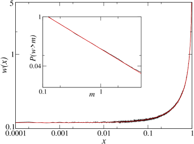
Figure 1: Exact results for the CCM model Mann04 is compared with numerical simulations. Practically they are indistinguishable. Main figure shows individual wealth of the agents arranged in a nondecreasing order of their saving propensity. The inset compares cumulative distribution of wealth. Parameters are $L=10^{4}$ and $N=10^{4}$.

The results discussed in Eq. (11) are valid for any $q$, where one expects $P(w)=C/w^{2}$. However, earlier numerical studies Bikas03 have reported a power-law distribution only for large $q$. The discrepancy can be explained as follows. The minimum wealth of the system is $w(0)=qC$ and the maximum is $w(1)=qC/(1-q^{2})$. The width of the interval $q^{3}C/(1-q^{2})$ is quite small for small $q$ unless $C$ is large. Since $C$ is proportional to $\bar{E}$ one must take large average wealth to see such a power law. Beacause of the finite lower limit in $w$, the cumulative distribution $P(w>m)=1-q^{-1}+C/n$ shows a power law up to a constant. We have plotted $P(w>m)+q^{-1}-1$ vs $m$ in logarithmic scale in Fig. 2 which perfectly fits to $C/m$ (see figure caption for details).

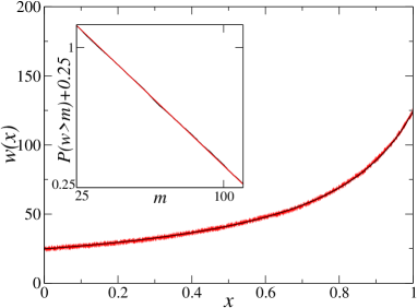
Figure 2: $w(x)$ obtained from simulations of a restricted saving model ($0<\lambda_{i}<q$) is plotted together with the exact result (11). Inset compares the cumulative distribution of wealth. Here $q=0.8$, $L=10^{4}=N$, and $\bar{E}=50$.

It is interesting to ask what happens when two different economies interact? For example take a system of $L$ agents, of which $q$ and $1-q$ fractions belong to two different organizations $\sigma=\pm$. Their saving propensity distributed according to $g_{\sigma}(\lambda)$, respectively, with $0<\lambda<1$. During trading agent $i$ of type $\sigma$ interacts with agent $j$ (type $\sigma^{\prime}$) and shares $\epsilon_{ij}(\sigma,\sigma^{\prime})$ and $1-\epsilon_{ij}(\sigma,\sigma^{\prime})$ fraction of ”available wealth”, respectively. Let us assume that $\langle\epsilon_{ij}(\sigma,\sigma^{\prime})\rangle=r_{\sigma\sigma^{\prime}}$ (obviously $r_{+-}=r_{-+}$). The distribution of the grand system is now $g(\lambda)=qg_{+}(\lambda)+pg_{-}(\lambda)$ and the effective sharing is $r=q^{2}r_{++}+(1-q)^{2}r_{--}+2q(1-q)r_{+-}.$ No matter what the value of $r$ is, Eq. (7) is still valid and thus the distribution of wealth is given by Eq. (9). So the power law $P(w)\sim w^{-2}$ and even Eq. (7) are quite robust.

Equation (7) is the central result of this paper, which states that the wealth of an agent having saving propensity $\lambda$ is inversely proportional to $1-\lambda$, irrespective of what the distribution $g(\lambda)$ and $h(\epsilon)$ are. It clearly indicates that on the average each agent, independent of how rich or poor he is, invests a constant wealth $C$ (which is of course $(1-\lambda$) fraction of his individual wealth) for trading lessC . And then with equal probability he receives $r$ or $1-r$ fraction of the available wealth $2C$. Thus, on the average, the individual wealth is preserved in the steady state.

One can instead write Eq. (7) as

$$w(\lambda)=\frac{C}{1-\lambda}~{}~{}\textrm{with}~{}~{}C^{-1}=\bar{E}^{-1}\int\frac{g(\lambda)d\lambda}{1-\lambda}$$ (12)

thus, better saving means better wealth. To verify the robustness of Eq. (12) let us divide the system of $L$ agents with their savings distributed uniformly in $(0,q)$ into two groups : (a) the poor savers who have $\lambda_{i}<z$ and (b) the rich savers who have $z\leq\lambda<q$. If the poor savers interact only with the poor and the rich savers interact only with the rich, clearly the system breaks up into two independent subsystems of size $zL$ and $(q-z)L$, respectively. Correspondingly wealth for the poor and the rich are $w_{p}(\lambda)=C_{p}/(1-\lambda)$ and $w_{r}(\lambda)=C_{r}/(1-\lambda)$, where $C_{p}$ and $C_{r}$ are to be determined independently from the initial average of wealth in each system. The total distribution of wealth is $P(w)=zP_{p}(w)+(q-z)P_{r}(w)$, where the distribution for the poor and the rich are $P_{r,p}(w)=C_{r,p}/w^{2}$, nonzero in the interval $w_{p}(0)<w<w_{p}(z)$, and $w_{r}(z)<w<w_{p}(1)$, respectively. Depending on the choice of parameters one can get different intervals where $P_{p}$, $P_{r}$ , both or none of them contribute to $P(w)$. For a certain choice, as described in the inset of Fig. 3, it is possible to obtain a cumulative wealth distribution which resembles the one observed in reality. Correspondingly a poor-rich break up at $\lambda=0.4$ is shown in Fig. 3(a). This discontinuity disappears once some intermediate savers (whose saving propensities are limited to $z<\lambda_{i}<b$) are introduced who can interact with both the poor and the rich savers. Surprisingly $w(\lambda)$ and $P(w)$ in this system are identical to that of the original CCM model where every agent interacts with every other agent. Fig. 3(b) compares $w(x)$ obtained from a numerical simulation for the poor-intermediate-rich system with the exact results. This suggests that that each agent in the system stands by their own. Irrespective of their distribution of saving propensity and interaction with other agents, any tagged agent who has saving propensity $\lambda$ acquires wealth which is inversely proportional to $(1-\lambda)$. Equation (12) is thus quite robust.

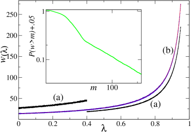
Figure 3: (a) $w(\lambda)$ for the poor-rich system, where poor savers own $2/3$ of the total wealth. Inset shows corresponding cumulative distribution of wealth. (b) $w(\lambda)$ for the poor-intermediate-rich model compared with CCM model Mann04 . Here $z=0.4$, $b=0.6$, $q=0.95$ and, $L=10^{4}=N$.

So far we have discussed the distribution of wealth in a ensemble of infinitely many identical systems. Instead, if we look at any given system which is a member of the ensemble, wealth of any particular agent (saving propensity $\lambda$) would show fluctuations about the average $w=C/(1-\lambda)$. Such fluctuations have been studied in MannaBook . These numerical studies indicate that the distribution of fluctuations $P(E)$ for any tagged agent (saving propensity $\lambda$) is a Gamma-like distribution which is asymmetric about the mean $w=C/(1-\lambda)$ and is peaked at $E_{c}<w$. It is also known that the distribution becomes symmetric with $E_{c}$ approaching $w$ when $\lambda\to 1$. Since usually agents are crowded around the peak of the distribution, in any particular system in the ensemble $P(E)$ is not very different from $P(E_{c})$. Thus for the rich (who have $\lambda\approx 1$), the distribution of wealth $P(E)$ is the same as $P(w)$ (as $E_{c}\approx w$), which explains the Pareto law for the rich in every system in a ensemble Patri05 . Whereas deviation of $P(E)$ from a power law is expected for the poor. An exact study of fluctuations could reveal the discrepancy.

What happens in a system of identical agents (each having same saving propensity $\lambda$)? Note that we need not consider identical copies of the systems now. The system itself is an ensemble of identical agents. Clearly the average wealth is $w=C/(1-\lambda)=\bar{E}$, and thus the probability distribution $P(w)=\delta(w-\bar{E})$. Agents in the system differ by their fluctuations and thus the distribution of wealth at any given instant would only count the fluctuations about the average $\bar{E}$, which is not different from the distribution of fluctuations of a tagged agent in CCM model. Extensive numerical simulations Bikas03 have shown a Gamma-like distribution in this case. Further analytic study might shed light on the exact form of distribution.

In conclusion, we have provided an exact solution to the ideal-gas-like markets using Gibbs ensemble approach. We point out that in a system of nonidentical agents, it is appropriate to consider infinitely many identical copies of the systems differing by their initial conditions. Such ensembles represent the evolution of several identical systems under the same macroscopic conditions and, thus, physical observables make sense only as an ensemble-averaged quantity. One single system, instead, would encounter fluctuations which are sometimes incalculably complex. A system of agents having the same saving propensity is such a case, where average quantities like wealth are identical for every agent and fluctuations are the only things that count. The central result revealed from our exact solution is that in ideal-gas-like markets, irrespective of the details of the interaction and distribution of saving propensity, an agent having saving propensity $\lambda$ would, on the average, acquire wealth which is inversely proportional to $1-\lambda$, $i.e.$, better savers are richer. Thus, every agent, poor ( small $\lambda$) or rich (large $\lambda$), on the average invests the same amount for trading, contrary to the real economy where rich agents usually invest more. To alter such scenario one might modify this minimal model so that the investment is non-linear in $w$ [note that current investment $(1-\lambda)w$ is linear].

I would like to acknowledge exciting discussions with B. K. Chakrabarti, K. Sengupta, R. Stinchcombe, A. Das, and A. Chatterjee.

References

- (1) V. Pareto, Cours d’economie Politique ( F. Rouge, lausanne, 1897).
- (2) A. A. Dragulescu and V. M. Yakovenko, Physica A 299, 213 (2001); W. Souma, Fractals 9, 463 (2001); T. Di Matteo, T. Aste and S. T. Hyde, cond-mat/0310544 and in ”The Physics of Complex Systems (New Advances and Perspectives)”, Eds. F. Mallamace and H. E. Stanley, (IOS Press, Amsterdam 2004); S. Sinha, Physica A 555 (2005); F. Clementi and M. Gallegati, Physica A 350, 427(2005).
- (3) A. A. Dragulescu and V. M. Yakovenko, Eur. Phys. J. B 17, 723 (2000).
- (4) A. Chakraborti and B. K. Chakrabarti, Eur. Phys. J. B 17, 167 (2000).
- (5) A. Chatterjee, B. K. Chakrabarti and S.S. Manna, Physica Scripta T106, 36 (2003); ibid Physica A 335, 155(2004).
- (6) M. Patriarca, A. Chakraborti and K. Kaski, Phys. Rev. E70, 016104 (2004).
- (7) P. Repetowicz, S. Hutzler and P. Richmond, Physica A 356, 641(2005).
- (8) Econophysics of Wealth Distribution Eds. A. Chatterjee, S. Yarlagadda and B. K. Chakrabarti, Springer Verlag, Milano 2005.
- (9) A. Das and S. Yarlagadda, Phys. Scripta T106, 39 (2003); A. Chatterjee, B. K. Chakrabarti, R. B. Stinchcombe, Phys. Rev. E 72 , 026126 (2005).
- (10) Note that no one posses lesser wealth than .
- (11) K. Bhattacharya, G. Mukherjee and S. S. Manna in Book ; Y. Fujiwara et. al., Physica A 321, 598(2004).
- (12) A similar arguement has been used by M. Patriarca, A. Chakraborti, K. Kaski and G. Germano in Book .