Nonrelativistic QED approach to the Lamb shift

Abstract

We calculate the one- and two-loop corrections of order $\alpha\,(Z\,\alpha)^{6}$ and $\alpha^{2}\,(Z\,\alpha)^{6}$ respectively, to the Lamb shift in hydrogen-like systems using the formalism of nonrelativistic quantum electrodynamics. We obtain general results valid for all hydrogenic states with nonvanishing orbital angular momentum and for the normalized difference of $S$-states. These results involve the expectation value of local effective operators and relativistic corrections to Bethe logarithms. The one-loop correction is in agreement with previous calculations for the particular cases of $S$, $P$, and $D$ states. The two-loop correction in the order $\alpha^{2}\,(Z\,\alpha)^{6}$ includes the pure two-loop self-energy and all diagrams with closed fermion loops. The obtained results allow one to obtain improved theoretical predictions for all excited hydrogenic states.

I Introduction

The precise calculation of the electron self-energy contribution to energy levels of hydrogen-like systems is a long-standing problem in bound-state quantum electrodynamics. The widely used direct numerical approach Mo1974a ; Mo1974b ; YeInSh2005 is based on a partial-wave decomposition of the Dirac-Coulomb propagator, which corresponds to the exact all-order treatment of the electron-nucleus interaction. The one-loop corrections have already been calculated to a high numerical precision for a wide range of nuclear charge numbers $Z$ (including the case of atomic hydrogen $Z=1$), whereas the two-loop correction has been obtained only for $Z\geq 10$ with limited numerical precision. The analytic method is based on an expansion in powers of $Z\,\alpha$ and a subsequent analytic or semianalytic integration. The two approaches are complementary. In practice, the numerical method has primarily been used for systems with a high nuclear charge number, whereas the analytic method usually provides more accurate predictions for low-$Z$ systems.

Here, we present a unified analytic derivation of the one- and two-loop binding corrections of order $(\alpha/\pi)\,(Z\,\alpha)^{6}m\,c^{2}$ and $(\alpha/\pi)^{2}\,(Z\,\alpha)^{6}m\,c^{2}$ respectively, for arbitrary bound states of hydrogen-like system using the formalism of dimensionally regularized nonrelativistic quantum electrodynamics (NRQED). This method allows for a natural separation of different energy scales, (i) the electron mass and (ii) the binding energy, using only one regularization parameter: the dimension $d$ of the coordinate space. This leads to a straightforward derivation of radiative corrections in terms of expectation values of some effective operators and the Bethe logarithms. The calculation of these operators is the main task of this work, and we obtain them from standard electromagnetic form factors and the low-energy limit of the two-photon exchange scattering amplitude.

This paper is organized as follows: In Sec. II, dimensionally regularized NRQED is outlined. In Sec. III, the one-loop self-energy is derived by splitting the calculation into low- (Sec. III.2), middle- (Sec. III.3), and high-energy parts. The general one-loop result is presented in Sec. III.4, and the evaluation for $D$, $P$ and $S$ states in Secs. III.5, III.6 and III.7, respectively. The two-loop correction is separated into four different gauge-invariant sets of diagrams, see Figs. 1—4 below. These are subsequently investigated in Secs. IV—VII. Results are summarized in Sec. IX. Moreover, in Appendix C we present the calculation of an additional two-loop logarithmic contribution to the ground state which was omitted in the previous work Pa2001 .

II Dimensionally regularized NRQED

As is customary in dimensionally regularized QED, we assume that the dimension of the space-time is $D=4-2\,\varepsilon$, and that of space $d=3-2\,\varepsilon$. The parameter $\varepsilon$ is considered as small, but only on the level of matrix elements, where an analytic continuation to a noninteger spatial dimension is allowed. Let us briefly discuss the extension of the basic formulas of NRQED to the case of an arbitrary number of dimensions. Some basis of dimensionally regularized NRQED in the context of hydrogen Lamb shift has already been formulated in PiSo1998 , however our approach presented below differs in many details.

The momentum-space representation of the photon propagator preserves its form, namely $g_{\mu\nu}/k^{2}$. The Coulomb interaction is

$$V(r) =-Z\,e^{2}\,\int\frac{d^{d}k}{(2\,\pi)^{d}}\,\frac{e^{{\rm i}\,\vec{k}\cdot\vec{r}}}{k^{2}}$$

$$=-\frac{Z\,e^{2}}{4\,\pi\,r^{1-2\,\varepsilon}}\,\left[(4\,\pi)^{\varepsilon}\,\frac{\Gamma(1-2\,\varepsilon)}{\Gamma(1-\varepsilon)}\right]\equiv-\frac{Z_{\varepsilon}\,\alpha}{r^{1-2\,\varepsilon}}\,,$$ (1)

where the latter representation provides an implicit definition of $Z_{\varepsilon}$, and we have used the formula for the surface area of a $d$-dimensional unit sphere

$$\Omega_{d}=\frac{2\,\pi^{d/2}}{\Gamma(d/2)}\,.$$ (2)

The nonrelativistic Hamiltonian of the hydrogenic system is

$$H=\frac{\vec{p}^{\;2}}{2\,m}-\frac{Z_{\varepsilon}\,\alpha}{r^{1-2\,\varepsilon}}\,.$$ (3)

We now turn to relativistic corrections to the Schrödinger Hamiltonian in an arbitrary number of dimensions. These corrections can be obtained from the Dirac Hamiltonian by the Foldy-Wouthuysen transformation. In order to incorporate a part of the radiative effects right from the beginning, we use an effective Dirac Hamiltonian modified by the electromagnetic form factors $F_{1}$ and $F_{2}$ (see, e.g., Chap. 7 of ItZu1980 ),

$$H_{D}= \vec{\alpha}\cdot\left[\vec{p}-e\,F_{1}(\vec{\nabla}^{2})\,\vec{A}\right]+\beta\,m+e\,F_{1}(\vec{\nabla}^{2})\,A_{0}$$

$$+F_{2}(\vec{\nabla}^{2})\,\frac{e}{2\,m}\,\left({\rm i}\,\vec{\gamma}\cdot\vec{E}-\frac{\beta}{2}\,\Sigma^{ij}\,B^{ij}\right)\,,$$ (4)

where

$$B^{ij} = \nabla^{i}\,A^{j}-\nabla^{j}\,A^{i}\,,$$ (5)

$$\nabla^{i} \equiv \nabla_{i}=\partial/\partial x^{i}\,,$$ (6)

$$\Sigma^{ij} = \frac{\rm i}{2}\,[\gamma^{i},\gamma^{j}]\,.$$ (7)

Formulas for the electromagnetic form factors $F_{1,2}$ can be found in Appendix A. Having the Foldy-Wouthuysen transformation defined by the operator $S$ (see Ref. Pa2004 ),

$$S= -\frac{\rm i}{2\,m}\,\left\{\beta\,\vec{\alpha}\cdot\vec{\pi}-\frac{1}{3\,m^{2}}\,\beta\,(\vec{\alpha}\cdot\vec{\pi})^{3}\right.$$

$$\left.+\frac{e(1+\kappa)}{2\,m}\,{\rm i}\,\vec{\alpha}\cdot\vec{E}-\frac{e\,\kappa}{8\,m^{2}}\,[\vec{\alpha}\cdot\vec{\pi},\beta\,\Sigma^{ij}\,B^{ij}]\right\}\,,$$ (8)

where $\kappa\equiv F_{2}(0)$, the new Hamiltonian is obtained via

$$H_{FW}=e^{{\rm i}\,S}\,(H_{D}-i\,\partial_{t})\,e^{-{\rm i}\,S}$$ (9a)

and takes the form

$$H_{FW}=\frac{\vec{\pi}^{\;2}}{2\,m}+e\,[1+F^{\prime}_{1}(0)\,{\vec{\nabla}}^{2}]A^{0}-\frac{e}{4\,m}\,(1+\kappa)\,\sigma^{ij}\,B^{ij}$$

$$-\frac{\vec{\pi}^{\;4}}{8\,m^{3}}-\frac{e}{8\,m^{2}}\,(1+2\,\kappa)\,\left[\vec{\nabla}\cdot\vec{E}+\sigma^{ij}\,\{E^{i},\pi^{j}\}\right]$$

$$-\frac{e}{8\,m^{4}}\,[F^{\prime}_{1}(0)+2\,F^{\prime}_{2}(0)]\,\vec{\nabla}^{2}\,\left[\vec{\nabla}\cdot\vec{E}+\sigma^{ij}\,\{E^{i},\pi^{j}\}\right]$$

$$+\frac{\vec{p}^{\,6}}{16\,m^{5}}+\frac{3+4\,\kappa}{64\,m^{4}}\,\bigl{\{}\vec{p}^{\;2},\vec{\nabla}\cdot\vec{E}+\sigma^{ij}\,\{E^{i},\pi^{j}\}\bigr{\}}$$

$$+\frac{4\,\kappa\,(1+\kappa)-1}{32\,m^{3}}\,e^{2}\,\vec{E}^{2}+\ldots$$ (9b)

The ellipsis denotes the omitted higher-order terms. We adopt the following conventions: $\{X,Y\}\equiv X\,Y+Y\,X$, $\vec{\pi}=\vec{p}-e\,\vec{A}$, $\sigma^{ij}=[\sigma^{i},\,\sigma^{j}]/(2\,{\rm i})$, and the form factors $F_{1}$, $F_{2}$ are defined in Eq. (106) below. In $d=3$ spatial dimensions, the matrices $\sigma^{ij}$ are equal to $\epsilon^{ijk}\,\sigma^{k}$. The electromagnetic field in $H_{FW}$ is the sum of the external Coulomb field and a slowly varying field of the radiation.

There is an additional correction that cannot be accounted for by the $F_{1}$ and $F_{2}$ form factors. It is represented by an effective local operator that is quadratic in the field strengths. This operator is derived separately by evaluating a low-energy limit of the electron scattering amplitude off the Coulomb field. An outline of this calculation are presented in Appendix B. The result is

$$\delta H=\frac{e^{2}}{m^{3}}\,\vec{E}^{\;2}\,\chi\,,$$ (10)

where $E$ is an electric field, and the functions $\chi\equiv\chi^{(1)}+\chi^{(2)}$ are given by Eq. (125).

III ONE–LOOP ELECTRON SELF–ENERGY

III.1 Brief outline of the calculation

The one-loop electron self-energy contribution in hydrogenlike atoms is

$$\delta^{(1)}E= \frac{e^{2}}{\rm i}\,\int\frac{d^{D}k}{(2\pi)^{D}}\,\frac{1}{k^{2}}$$

$$\times\left<\bar{\psi}\left|\gamma^{\mu}\,\frac{1}{\not\!p-\not\!k-m-\gamma^{0}\,V}\,\gamma_{\mu}\right|\psi\right>$$

$$-\delta m\,\langle\bar{\psi}|\psi\rangle\,.$$ (11)

Here, $p^{0}=E_{\psi}$ is the Dirac energy of the reference state, $V$ is the Coulomb potential in $d$ dimensions, and we use natural relativistic units with $\hbar=c=\epsilon_{0}=1$, so that $e^{2}=4\pi\alpha$. The electron mass is denoted by $m$, and $\delta m$ is the one-loop mass counter term. By $\psi$ we denote the Dirac wave function. There are three energy scales in Eq. (11), which imply a natural separation of the one-loop $\delta^{(1)}E$ into three parts,

$$\delta^{(1)}E=E_{L}+E_{M}+E_{H}\,.$$ (12)

Each part is regularized separately using the same dimensional regularization. $E_{L}$ is the low energy part, where the photon momentum is of order $k\sim(Z\,\alpha)^{2}\,m$. $E_{M}$ is the middle-energy part, where $k\sim m$, and the electron momentum is $p\sim(Z\,\alpha)\,m$. Finally, $E_{H}$ is a high-energy part where all loop momenta are of the order of the electron mass. It is given by the forward three-Coulomb scattering amplitude and is represented as a local interaction, proportional to $\delta^{d}(r)$.

The naming convention for the high-, middle-, and low-energy parts is a little different from our previous convention. E.g., in  Pa1993 , the contribution referred to as the “high-energy part” in this reference would correspond to the sum of the “high-energy part” and the “middle-energy part” in the context of the current evaluation. The renaming of the contributions is influenced by the NRQED-approach used here and by the correspondence of the different parts to specific effective operators. In this work, for all operators $Q$, we consider only the expectation values for states with

$$l\neq 0,$$ (13a)

and the normalized difference of expectation values

$$\left<\!\left<Q\right>\!\right>\equiv n^{3}\,\left<nS|Q|nS\right>-\left<1S|Q|1S\right>$$ (13b)

for $S$ states. For this reason the high-energy part $E_{H}$ vanishes here. Consequently the “middle-energy part” as considered in the current investigation corresponds exactly to the “high-energy part” of Refs. JePa1996 ; JeSoMo1997 .

The one-loop bound-state self-energy, for the states under consideration can be written as

$$\delta^{(1)}E\!=\!\frac{\alpha}{\pi}\frac{(Z\alpha)^{4}}{n^{3}}\left\{A_{40}+(Z\alpha)^{2}\left[A_{61}\ln[(Z\alpha)^{-2}]+A_{60}\right]\right\},$$ (14)

where the indices of the coefficients indicate the power of $Z\,\alpha$ and the power of the logarithm, respectively. The coefficient $A_{40}$ is well known (for reviews see e.g. EiGrSh2001 ; MoTa2005 ), and we focus here on derivation of the general expression for the $\alpha\,(Z\,\alpha)^{6}$ term.

III.2 Low-energy part

In the low energy part, all electron momenta are of the order of $Z\,\alpha$, so in principle, one could perform a direct nonrelativistic expansion of the matrix element

$$\left<\bar{\psi}\left|\gamma^{\mu}\,\frac{1}{\not\!p-\not\!k-m-\gamma^{0}\,V}\,\gamma_{\mu}\right|\psi\right>$$ (15)

that enters into Eq. (11). It is more convenient however, instead of using Eq. (11), to take the Dirac Hamiltonian with an electromagnetic field and to perform this expansion by applying the Foldy-Wouthuysen transformation. The resulting Hamiltonian, in $d$ dimensions, is given in Eq. (9). Here, we can neglect form factors and $H_{FW}$ becomes (from now on we will set the electron mass $m$ equal to unity)

$$H_{FW}=\frac{\vec{\pi}^{\,2}}{2}+V(r)-\frac{e}{4}\,\sigma^{ij}\,B^{ij}-\frac{\vec{\pi}^{\,4}}{8}+\frac{\pi}{2}\,Z\,\alpha\,\delta^{d}(r)$$

$$+\frac{1}{4}\,\sigma^{ij}\,\nabla^{i}V\,\pi^{j}-\frac{e}{8}\,\Bigl{[}\vec{\nabla}\cdot\vec{E}+\sigma^{ij}\,(E^{i}\,\pi^{j}+\pi^{j}\,E^{i})\Bigr{]}\,.$$ (16)

The contribution from the Coulomb potential $V$ is explicitly separated from the additional electromagnetic fields $\vec{E}$ and $\vec{B}$. The Hamiltonian in Eq. (III.2) may be used to derive the low-energy part which receives a natural interpretation as the sum of various relativistic corrections to the Bethe logarithm. We use the Coulomb gauge for the photon propagator, and only the transverse part will contribute. This treatment of the low-energy part is similar to previous calculations Pa1993 ; JePa1996 , the difference lies in the presence of dimensional regularization.

The leading nonrelativistic (dipole) low-energy contribution is

$$E_{L0} = e^{2}\int\frac{d^{d}k}{(2\,\pi)^{d}\,2\,k}\,\left(\delta^{ij}-\frac{k^{i}\,k^{j}}{k^{2}}\right)\,$$ (17)

$$\times\left<\phi\left|p^{i}\,\frac{1}{E-H-k}\,p^{j}\right|\phi\right>\,,$$

where by $H$ we denote the nonrelativistic Hamiltonian in $d$ dimensions, Eq. (3). The wave function $\phi$, in contrast to $\psi$ [see Eq. (11)], denotes the nonrelativistic Schrödinger–Pauli wave function. In the following, we will denote the expectation value of an arbitrary operator $Q$, evaluated with the nonrelativistic Schrödinger–Pauli wave function, by the shorthand notation $\langle Q\rangle$.

After the $d$-dimensional integration with respect to $k$, and the expansion in $\varepsilon$, $E_{L0}$ becomes PiSo1998

$$E_{L0} = (4\,\pi)^{\varepsilon}\,\Gamma(1+\varepsilon)\,\frac{2\,\alpha}{3\,\pi}\,$$

$$\times\left<\vec{p}\,(H-E)\left\{\frac{1}{2\,\varepsilon}+\frac{5}{6}-\ln\left[2(H-E)\right]\right\}\vec{p}\,\right>\,,$$

where we ignore terms of order $\varepsilon$ and higher. Because the factor $(4\,\pi)^{\varepsilon}\,\Gamma(1+\varepsilon)$ appears in all the terms, we will drop it out consistently in the low-, middle- and high-energy parts, and as well as in the form factors. Moreover, in the two-loop calculations discussed below, we will drop the square of this factor. The contribution $E_{L0}$ can be rewritten as

$$E_{L0} = \frac{4\,\alpha}{3}\,Z\,\alpha\,\left\{\frac{1}{2\,\varepsilon}+\frac{5}{6}+\ln[(Z\,\alpha)^{-2}]\right\}\,\langle\delta^{d}(r)\rangle$$ (19)

$$-\frac{4\alpha}{3\pi}\,\frac{(Z\,\alpha)^{4}}{n^{3}}\,\ln k_{0}\,,$$

where the second term in this equation involves the Bethe logarithm $\ln k_{0}$ defined as

$$\frac{(Z\,\alpha)^{4}}{n^{3}}\,\ln k_{0}=\frac{1}{2}\,\left<\vec{p}\,(H-E)\,\ln\left[\frac{2(H-E)}{(Z\,\alpha)^{2}}\right]\,\vec{p}\,\right>\,.$$ (20)

We consider now all possible relativistic corrections to Eq. (19), and introduce the notation

$$\delta_{Q}\,\left<p^{i}\,\frac{1}{E-H-k}\,p^{j}\right>\equiv\biggl{<}p^{i}\,\frac{1}{E-H-k}\,(Q-\langle Q\rangle)\,$$

$$\frac{1}{E-H-k}\,p^{j}\biggr{>}+2\,\left<Q\,\frac{1}{(E-H)^{\prime}}\,p^{i}\,\frac{1}{E-H-k}\,p^{j}\right>\,,$$ (21)

where $Q$ is an arbitrary operator. $\delta_{Q}$ involves the first-order perturbations to the Hamiltonian, to the energy, and to the wave function. The first correction $E_{L1}$ is the modification of $E_{L0}$ by the relativistic correction to the Hamiltonian,

$$H_{R}=-\frac{\vec{p}^{\,4}}{8}+\frac{\pi}{2}\,Z\,\alpha\,\delta^{d}(r)+\frac{1}{4}\,\sigma^{ij}\,\nabla^{i}V\,p^{j}\,,$$ (22)

where $\delta^{d}(r)$ is a $d$-dimensional Dirac delta function. One could obtain $E_{L1}$ by including this $H_{R}$ in Eq. (19). However, for the comparison with former calculations and for convenience we will return to Eq. (17), and split $E_{L1}$ by introducing an intermediate cutoff $\Lambda$

$$E_{L1} = e^{2}\left(\int_{0}^{\Lambda}+\int_{\Lambda}^{\infty}\right)\frac{d^{d}k}{(2\,\pi)^{d}\,2\,k}\,\left(\delta^{ij}-\frac{k^{i}\,k^{j}}{k^{2}}\right)\,$$ (23)

$$\times\delta_{H_{R}}\left<p^{i}\,\frac{1}{E-H-k}\,p^{j}\right>\,.$$

After the $Z\,\alpha$ expansion with $\Lambda=\lambda\,(Z\,\alpha)^{2}$, one goes subsequently to the limits $\varepsilon\rightarrow 0$ and $\lambda\rightarrow\infty$. Under the assumptions (13), we may perform an expansion in $1/k$ in the second part and obtain

$$E_{L1}=\frac{2\,\alpha}{3\,\pi}\,\int_{0}^{\Lambda}dk\,k\,\delta_{H_{R}}\left<\,\vec{p}\,\frac{1}{E-H-k}\,\vec{p}\,\right>$$ (24)

$$+\frac{\alpha}{3\,\pi}\,\left[1+\varepsilon\,\left(\frac{5}{3}-2\,\ln 2\right)\right]\,\int_{\Lambda}^{\infty}dk\,\frac{1}{k^{1+2\,\varepsilon}}\,$$

$$\left\{\left<[\,\vec{p},[\,H_{R},\vec{p}\,]]\right>+2\,\left<H_{R}\,\frac{1}{(E-H)^{\prime}}\,[\,\vec{p},[\,H,\vec{p}\,]]\right>\right\}\,.$$

After performing the $k$-integration and with the help of commutator relations it reads

$$E_{L1} = \frac{\alpha}{\pi}\,\frac{(Z\,\alpha)^{6}}{n^{3}}\,\beta_{1}+\frac{\alpha}{3\,\pi}\,\left\{\frac{1}{2\,\varepsilon}+\frac{5}{6}+\ln\left[{\textstyle{\frac{1}{2}}}\,(Z\,\alpha)^{-2}\right]\right\}$$ (25)

$$\times\biggl{\{}\left<\frac{1}{8}\,\vec{\nabla}^{4}V+\frac{\rm i}{4}\,\sigma^{ij}\,p^{i}\vec{\nabla}^{2}V\,p^{j}\right>$$

$$+2\,\left<H_{R}\,\frac{1}{(E-H)^{\prime}}\,\vec{\nabla}^{2}V\right>\biggr{\}}\,.$$

Here, $\beta_{1}$ is a dimensionless quantity, defined as a finite part of the $k$-integral with divergent terms proportional to $\lambda^{n}$ ($n=1,2,\dots$) and $\ln(\lambda)$ dropped out in the limit of large $\lambda$,

$$\frac{\alpha}{\pi}\,\frac{(Z\,\alpha)^{6}}{n^{3}}\,\beta_{1} = \lim_{\lambda\rightarrow\infty}\frac{2\,\alpha}{3\,\pi}\,\int_{0}^{\Lambda}dk\,k\,$$ (26)

$$\times\delta_{H_{R}}\,\left<p^{i}\,\frac{1}{E-H-k}\,p^{i}\right>\,,$$

We recall the relation $\Lambda=\lambda\,(Z\,\alpha)^{2}$. In all integrals with an upper limit $\Lambda$ to be discussed in the following, the divergent terms in $\lambda$ will be subtracted. Following earlier treatments (e.g., JeEtAl2003 ), we subtract exactly the term proportional to $\ln(\lambda)$, but not $\ln(2\,\lambda)$. The presence of the factor ${\textstyle{\frac{1}{2}}}$ under the logarithm in Eq. (25) is a consequence of this subtraction.

The quantity $\beta_{1}$ can only be calculated numerically. In constitutes one of three contributions to relativistic Bethe logarithm $\cal L$, being defined as in JeEtAl2003 .

$${\cal L}=\beta_{1}+\beta_{2}+\beta_{3}\,.$$ (27)

Two others $\beta_{2}$, $\beta_{3}$ are defined in Eqs. (III.2) and (35) below. In this sense, the definition of $\beta_{1}$ in Eq. (26) corresponds to the definition of the low energy part ${\cal L}$ in Eq. (9) of Ref. JeEtAl2003 .

The second relativistic correction $E_{L2}$ is the nonrelativistic quadrupole contribution in the conventions adopted in Pa1993 ; JePa1996 . Specifically, it is the quadratic (in $k$) term from the expansion of $\exp({\rm i}\,\vec{k}\cdot\vec{r})$,

$$E_{L2} = e^{2}\int\frac{d^{d}k}{(2\,\pi)^{d}\,2\,k}\,\left(\delta^{ij}-\frac{k^{i}\,k^{j}}{k^{2}}\right)\,$$ (28)

$$\times\biggl{[}\left<p^{i}\,({\rm i}\,\vec{k}\cdot\vec{r})\,\frac{1}{E-H-k}\,p^{j}\,(-{\rm i}\,\vec{k}\cdot\vec{r})\right>$$

$$+\left<p^{i}\,({\rm i}\,\vec{k}\cdot\vec{r})^{2}\,\frac{1}{E-H-k}\,p^{j}\right>\biggr{]}\,.$$

In a similar way as for $E_{L1}$, we split the integration into two parts, by introducing a cutoff $\Lambda$. In the first part, with the $k$-integral from $0$ to $\Lambda$, one can set $d=3$ and extract the logarithmic divergence. In the second part, with the $k$-integral from $\Lambda$ to $\infty$, we perform a $1/k$ expansion and employ commutator relations, with the intent of moving the operator $H-E$ to the far left or right where it vanishes when acting on the Schrödinger–Pauli wave function. In this way we obtain

$$E_{L2} = \frac{\alpha}{\pi}\,\frac{(Z\,\alpha)^{6}}{n^{3}}\,\beta_{2}+\frac{\alpha}{\pi}\,\left<(\vec{\nabla}V)^{2}\,\frac{2}{3}\,\left[\frac{1}{\varepsilon}+\frac{103}{60}+2\,\ln\left[{\textstyle{\frac{1}{2}}}\,(Z\,\alpha)^{-2}\right]\right]\right.$$ (29)

$$\left.+\vec{\nabla}^{4}V\,\frac{1}{40}\,\left[\frac{1}{\varepsilon}+\frac{12}{5}+2\,\ln\left[{\textstyle{\frac{1}{2}}}\,(Z\,\alpha)^{-2}\right]\right]+\vec{\nabla}^{2}V\,\vec{p}^{\,2}\,\frac{1}{6}\,\left[\frac{1}{\varepsilon}+\frac{34}{15}+2\,\ln\left[{\textstyle{\frac{1}{2}}}\,(Z\,\alpha)^{-2}\right]\right]\right>\,.$$

Here, $\beta_{2}$ is defined as the finite part of the integral [see the discussion following Eq. (26)]

$$\frac{\alpha}{\pi}\,\frac{(Z\,\alpha)^{6}}{n^{3}}\,\beta_{2}=4\,\pi\,\alpha\,\,\lim_{\lambda\rightarrow\infty}\int_{0}^{\Lambda}\frac{d^{3}k}{(2\,\pi)^{3}\,2\,k}\,\left(\delta^{ij}-\frac{k^{i}\,k^{j}}{k^{2}}\right)\,\left\{\left<\,p^{i}\,({\rm i}\,\vec{k}\cdot\vec{r})^{2}\,\frac{1}{E-H-k}\,p^{j}\,\right>\right.$$

$$\left.+\left<\,p^{i}\,({\rm i}\,\vec{k}\cdot\vec{r})\,\frac{1}{E-H-k}\,p^{j}\,(-{\rm i}\,\vec{k}\cdot\vec{r})\,\right>\right\}\,.$$ (30)

The third contribution $E_{L3}$ originates from the relativistic corrections to the coupling of the electron to the electromagnetic field. These corrections can be obtained from the Hamiltonian in Eq. (1), and they have the form of a correction to the current

$$\delta j^{i}=-\frac{1}{2}\,p^{i}\,\vec{p}^{\,2}+\frac{1}{2}\,\sigma^{ij}\,k^{j}\,\vec{k}\cdot\vec{r}+\frac{\rm i}{4}\,\sigma^{ij}\,k\,p^{j}-\frac{1}{4}\,\sigma^{ij}\,\nabla^{j}V\,.$$ (31)

The corresponding correction $E_{L3}$ is

$$E_{L3} = 2\,e^{2}\int\frac{d^{d}k}{(2\,\pi)^{d}\,2\,k}\,\left(\delta^{ij}-\frac{k^{i}\,k^{j}}{k^{2}}\right)\,\left<\delta j^{i}\frac{1}{E-H-k}\,p^{j}\right>\,.$$ (32)

We now perform an angular averaging of the matrix element, replace $k$ in the numerator by $E-H$, and use commutator relations to bring the correction $E_{L3}$ into the form

$$E_{L3}=-2\,e^{2}\,\frac{d-1}{d}\,\int\frac{d^{d}k}{(2\,\pi)^{d}\,2\,k}\,\left<\left(\frac{p^{k}\,{\vec{p}}^{\,2}}{2}+\frac{d-2}{d-1}\,\frac{\sigma^{kl}\,\nabla^{l}V}{2}\right)\frac{1}{E-H-k}\,p^{k}\right>\,.$$ (33)

We again split this integral into two parts. In the first part $k<\Lambda$, one can approach the limit $d=3$, and in the second part $k>\Lambda$ one performs a $1/k$-expansion and obtains

$$E_{L3} = \frac{\alpha}{\pi}\,\frac{(Z\,\alpha)^{6}}{n^{3}}\,\beta_{3}-\frac{4\alpha}{3\,\pi}\,\left[\frac{1}{2\,\varepsilon}+\frac{5}{6}+\ln\left[{\textstyle{\frac{1}{2}}}\,(Z\,\alpha)^{-2}\right]\right]\left<\frac{1}{4}\,\vec{\nabla}^{2}V\,\vec{p}^{\,2}+\frac{1}{2}\,\bigl{(}\vec{\nabla}V\bigr{)}^{2}\right>\,,$$ (34)

where $\beta_{3}$ is the finite part of the integral

$$\frac{\alpha}{\pi}\,\frac{(Z\,\alpha)^{6}}{n^{3}}\,\beta_{3}=-\frac{4\,\alpha}{3\,\pi}\,\lim_{\lambda\rightarrow\infty}\int_{0}^{\Lambda}dk\,k\left<\left(\frac{1}{2}\,p^{i}\,p^{2}+\frac{1}{4}\,\sigma^{ij}\,\nabla^{j}V\right)\,\frac{1}{E-H-k}\,p^{i}\,\right>\,.$$ (35)

This completes the treatment of the low energy part, which is

$$E_{L}=E_{L1}+E_{L2}+E_{L3}\,.$$ (36)

III.3 Middle-energy part

We here consider the middle-energy part $E_{M}$ as the contribution originating from photon momentum of the order of the electron mass and electron momenta of order $Z\,\alpha$. In this momentum region, radiative corrections can be effectively represented by electron form factors and higher-order structure functions. Electron form factors $F_{1}$ and $F_{2}$ modify the coupling of the Dirac electron to the electromagnetic field and the resulting effective Hamiltonian is given in Eq. (II). Here we assume that $\vec{A}=0$, $A^{0}$ represents a static Coulomb potential, and $\vec{E}=-\vec{\nabla}A^{0}$ is the electric field of the nucleus. One finds a nonrelativistic expansion by the Foldy-Wouthuysen transformation in Eq. (8), and the resulting Hamiltonian [see Eq. (9)] after putting $\vec{A}=0$ and neglecting $F_{2}(0)^{2}$ is

$$H_{FW} = \frac{\vec{p}^{\,2}}{2}+e\,F_{1}(\vec{\nabla}^{2})\,A^{0}-\frac{\vec{p}^{\,4}}{8}-\frac{e}{8}\,[F_{1}(\vec{\nabla}^{2})+2\,F_{2}(\vec{\nabla}^{2})]\,\Bigl{(}\vec{\nabla}\cdot\vec{E}+2\,\sigma^{ij}\,E^{i}\,p^{j}\Bigr{)}$$ (37)

$$+\frac{\vec{p}^{\,6}}{16}+\frac{e}{64}\,[3+4\,F_{2}(0)]\Bigl{\{}\vec{p}^{\,2},\vec{\nabla}\cdot\vec{E}+2\,\sigma^{ij}\,E^{i}\,p^{j}\Bigr{\}}-\frac{1-4\,F_{2}(0)}{32}\,e^{2}\,\vec{E}^{2}\,.$$

The leading $(\alpha/\pi)\,(Z\,\alpha)^{4}$ one-loop correction reads

$$E_{M0}=\langle\delta^{\rm(1)}V\rangle\,,$$ (38)

where the “radiative potential” $\delta V$ is defined as

$$\delta V=\left[F^{\prime}_{1}(0)+\frac{1}{4}\,F_{2}(0)\right]\,\vec{\nabla}^{2}V+\frac{F_{2}(0)}{2}\,\sigma^{ij}\,\nabla^{i}V\,p^{j}\,,$$ (39)

and the superscript ${\rm(1)}$ in Eq. (38) denotes the one-loop component of $\delta V$. The expansion of $F_{i}$ in powers of $q^{2}$ is obtained in Eq. (108). Using these results, one obtains

$$E_{M0}=-\frac{1}{6\,\varepsilon}\,\frac{\alpha}{\pi}\,\langle\vec{\nabla}^{2}V\rangle+\frac{\alpha}{4\,\pi}\,\langle\sigma^{ij}\nabla^{i}V\,p^{j}\rangle\,.$$ (40)

Together with the low-energy part $E_{L0}$ in Eq. (19), this gives

$$E_{0}\equiv E_{L0}+E_{M0} = \frac{\alpha}{\pi}\,(Z\,\alpha)^{4}\,\left[\frac{10}{9}+\frac{4}{3}\,\ln\left[(Z\,\alpha)^{-2}\right]\right]\,\frac{\delta_{l0}}{n^{3}}+\frac{\alpha}{4\,\pi}\,\left<\sigma^{ij}\nabla^{i}V\,p^{j}\right>-\frac{4\,\alpha}{3\,\pi}\,\frac{(Z\,\alpha)^{4}}{n^{3}}\,\ln k_{0}\,,$$ (41)

which is the well-known leading $(\alpha/\pi)\,(Z\,\alpha)^{4}$ contribution to the hydrogen Lamb shift.

Let us now consider the one-loop correction of relative-order $(Z\,\alpha)^{2}$. The first contribution $E_{M1}$ comes from the one-loop form factors $F_{1}$ and $F_{2}$ in Eq. (9) combined with the relativistic correction to the wave function:

$$E_{M1} = 2\,\left<\left\{\left[F^{\prime\rm(1)}_{1}(0)+\frac{1}{4}\,F^{\rm(1)}_{2}(0)\right]\,\vec{\nabla}^{2}V+\frac{F_{2}^{\rm(1)}(0)}{2}\,\sigma^{ij}\,\nabla^{i}V\,p^{j}\right\}\,\frac{1}{(E-H)^{\prime}}\,H_{R}\right>$$ (42)

$$+\frac{F^{\prime\rm(1)}_{1}(0)+2F^{\prime\rm(1)}_{2}(0)}{8}\,\langle\vec{\nabla}^{4}V+2\,{\rm i}\,\sigma^{ij}\,p^{i}\vec{\nabla}^{2}V\,p^{j}\rangle+F^{\prime\prime\rm(1)}_{1}(0)\,\langle\vec{\nabla}^{4}V\rangle$$

$$-\frac{F^{\rm(1)}_{2}(0)}{16}\,\left<\Bigl{\{}\vec{p}^{\,2},\vec{\nabla}^{2}V+2\,\sigma^{ij}\,\nabla^{i}V\,p^{j}\Bigr{\}}\right>+\frac{F^{\rm(1)}_{2}(0)}{8}\,\langle(\vec{\nabla}V)^{2}\rangle\,.$$

By the superscript (1), we denote the one-loop component of the form factors, as given in Eq. (107) in Appendix A.

The second contribution $E_{M2}$ comes from an additional term $\delta^{(1)}H$ in the NRQED Hamiltonian, see Eq. (10),

$$\delta^{\rm(1)}H=\left(\frac{1}{6}-\frac{1}{3\,\varepsilon}\right)\,\frac{\alpha}{\pi}\,(\vec{\nabla}V)^{2}\,.$$ (43)

The corresponding correction to the energy is

$$E_{M2}=\left<\delta^{\rm(1)}H\right>\,,$$ (44)

and the total $E_{M}$ contribution is

$$E_{M}=E_{M1}+E_{M2}\,.$$ (45)

III.4 General one-loop result

We may now present the complete one-loop correction $\delta^{\rm(1)}E$ up to the order $(\alpha/\pi)\,(Z\,\alpha)^{6}$. It is a sum of the low-energy term $E_{L}$ given in Eq. (36), the middle-energy term $E_{M}$ in Eq. (45), and the lower-order term $E_{0}$ as defined in Eq. (41),

$$\delta^{\rm(1)}E = \frac{\alpha}{\pi}\,\frac{(Z\,\alpha)^{4}}{n^{3}}\,\left\{\left[\frac{10}{9}+\frac{4}{3}\,\ln\left[(Z\,\alpha)^{-2}\right]\right]\,\delta_{l0}-\frac{4}{3}\,\ln k_{0}\right\}+\frac{Z\,\alpha^{2}}{4\,\pi}\,\left<\sigma^{ij}\nabla^{i}Vp^{j}\right>$$ (46)

$$+\frac{\alpha}{\pi}\,\left\{\frac{(Z\,\alpha)^{6}}{n^{3}}\,{\cal L}+\left(\frac{5}{9}+\frac{2}{3}\,\ln\left[{\textstyle{\frac{1}{2}}}\,(Z\,\alpha)^{-2}\right]\right)\,\left<\vec{\nabla}^{2}V\,\frac{1}{(E-H)^{\prime}}\,H_{R}\right>+\frac{1}{2}\,\left<\sigma^{ij}\nabla^{i}Vp^{j}\,\frac{1}{(E-H)^{\prime}}\,H_{R}\right>\right.$$

$$+\left(\frac{779}{14400}+\frac{11}{120}\,\ln\left[{\textstyle{\frac{1}{2}}}\,(Z\,\alpha)^{-2}\right]\right)\,\langle\vec{\nabla}^{4}V\rangle+\left(\frac{23}{576}+\frac{1}{24}\,\ln\left[{\textstyle{\frac{1}{2}}}\,(Z\,\alpha)^{2}\right]\right)\,\langle 2\,{\rm i}\,\sigma^{ij}\,p^{i}\vec{\nabla}^{2}Vp^{j}\rangle$$

$$+\left.\left(\frac{589}{720}+\frac{2}{3}\,\ln\left[{\textstyle{\frac{1}{2}}}\,(Z\,\alpha)^{2}\right]\right)\,\langle(\vec{\nabla}V)^{2}\rangle+\frac{3}{80}\,\bigl{\langle}\vec{p}^{\,2}\,\vec{\nabla}^{2}V\bigr{\rangle}-\frac{1}{8}\,\bigl{\langle}\vec{p}^{\,2}\,\sigma^{ij}\,\nabla^{i}Vp^{j}\bigr{\rangle}\right\}\,.$$

The first two terms corresponds to the $\alpha\,(Z\,\alpha)^{4}$ term in Eq. (14), whereas the latter terms give the $\alpha\,(Z\,\alpha)^{6}$ contribution. The relativistic Bethe Logarithm ${\cal L}$, defined in Eq. (27), consists of a sum of $\beta_{1}$ defined in Eq. (26), $\beta_{2}$ in Eq. (III.2), and $\beta_{3}$ in Eq. (35). For the convenience of the reader we briefly recall that all matrix elements should be evaluated in $d=3$ spacetime dimensions, which implies

$$\vec{\nabla}^{2}V \to 4\pi Z\,\alpha\,\delta^{3}(r)\,,$$ (47a)

$$\sigma^{ij}\nabla^{i}Vp^{j} \to Z\,\alpha\,\frac{\vec{\sigma}\cdot\vec{L}}{r^{3}}\,,$$ (47b)

$$\sigma^{ij}p^{i}\nabla^{2}Vp^{j} \to 4\pi Z\,\alpha\,\vec{p}\times[\delta^{3}(r)\vec{p}]\,,$$ (47c)

$$\sigma^{ij}\nabla^{j}V \to Z\,\alpha\frac{\vec{r}\times\vec{\sigma}}{r^{3}}\,.$$ (47d)

This concludes the calculation of the one-loop electron self-energy. The matrix elements entering into (46) are evaluated below in Secs. III.5, III.6, and III.7 for a number of hydrogenic states and compared to results previously obtained in the literature.

III.5 Results for $D$ states

Our aim is to give a few numerical results for some phenomenologically important hydrogenic states, based on the general result (46). For $D$ states, the wave function behaves at the origin as $\sim r^{2}$. This means that a few matrix elements, such as $\langle\vec{\nabla}^{4}V\rangle$, are actually vanishing. The following is a list of the nonvanishing matrix elements for $l=2$:

$$\left<nD\left|\frac{Z\,\alpha}{r^{3}}\,\frac{1}{(E-H)^{\prime}}\,\vec{p}^{\,4}\right|nD\right>$$

$$\qquad=\frac{(Z\,\alpha)^{6}}{n^{3}}\,\left(-\frac{1118}{7875}-\frac{4}{25\,n}+\frac{86}{105\,n^{2}}\right)\,,$$ (48a)

$$\left<nD\left|\frac{Z\,\alpha}{r^{3}}\,\frac{1}{(E-H)^{\prime}}\,\frac{Z\,\alpha}{r^{3}}\right|nD\right>$$

$$\qquad=\frac{(Z\,\alpha)^{6}}{n^{3}}\,\left(-\frac{709}{94500}-\frac{1}{150\,n}+\frac{1}{105\,n^{2}}\right)\,,$$ (48b)

$$\left<nD\left|\frac{(Z\,\alpha)^{2}}{r^{4}}\right|nD\right>=\frac{(Z\,\alpha)^{6}}{n^{3}}\,\frac{2(n^{2}-2)}{105\,n^{2}}\,,$$ (48c)

$$\left<nD\left|\vec{p}^{\,2}\,\frac{Z\,\alpha}{r^{3}}\right|nD\right>=\frac{(Z\,\alpha)^{6}}{n^{3}}\,\left(\frac{4}{105}-\frac{1}{7\,n^{2}}\right)\,.$$ (48d)

All of the above are evaluated on the nonrelativistic Schrödinger wave function. They are finite so that one may set the space dimension equal to three. The final results for the different fine-structure sublevels are

$$A_{60}(nD_{3/2})+A_{61}(nD_{3/2})\ln\left[(Z\alpha)^{-2}\right]$$

$$\qquad={\cal L}(nD_{3/2})-\frac{157}{30240}-\frac{3}{80n}+\frac{3007}{37800n^{2}}$$

$$\qquad\qquad+\frac{4}{315}\,\left(1-\frac{2}{n^{2}}\right)\ln\left[{\textstyle{\frac{1}{2}}}(Z\,\alpha)^{-2}\right],$$ (49a)

and

$$A_{60}(nD_{5/2})+A_{61}(nD_{5/2})\ln\left[(Z\alpha)^{-2}\right]$$

$$\qquad={\cal L}(nD_{5/2})+\frac{379}{18900}+\frac{1}{60n}-\frac{1759}{18900n^{2}}$$

$$\qquad\qquad+\frac{4}{315}\,\left(1-\frac{2}{n^{2}}\right)\ln\left[{\textstyle{\frac{1}{2}}}(Z\alpha)^{-2}\right].$$ (49b)

They are in agreement with results reported previously in Eqs. (12c) and (12d) of JeEtAl2003 . Values for ${\cal L}(nD_{3/2})$ and ${\cal L}(nD_{5/2})$ can be found in Table 1 of Ref. JeEtAl2003 .

III.6 Results for $P$ states

For $P$ states, a few more of the matrix elements in Eq. (46) are nonvanishing, and we have

$$\left<nP\left|\frac{Z\,\alpha}{r^{3}}\,\frac{1}{(E-H)^{\prime}}\,\vec{p}^{\,4}\right|nP\right>$$

$$\qquad=\frac{(Z\,\alpha)^{6}}{n^{3}}\,\left(-\frac{346}{135}-\frac{4}{3\,n}+\frac{22}{5\,n^{2}}\right)\,,$$ (50a)

$$\left<nP\left|\frac{Z\,\alpha}{r^{3}}\,\frac{1}{(E-H)^{\prime}}\,\frac{Z\,\alpha}{r^{3}}\right|nP\right>=$$

$$\qquad=\frac{(Z\,\alpha)^{6}}{n^{3}}\,\left(-\frac{227}{540}-\frac{1}{6\,n}+\frac{1}{5\,n^{2}}\right)\,,$$ (50b)

$$\left<nP\left|\frac{(Z\,\alpha)^{2}}{r^{4}}\right|nP\right>=\frac{(Z\,\alpha)^{6}}{n^{3}}\,\frac{2\,(3\,n^{2}-2)}{15\,n^{2}}\,,$$ (50c)

$$\left<nP\left|\vec{p}^{\,2}\,\frac{Z\,\alpha}{r^{3}}\right|nP\right>=\frac{(Z\,\alpha)^{6}}{n^{3}}\,\left(\frac{4}{5}-\frac{13}{15\,n^{2}}\right)\,,$$ (50d)

$$\left<nP\left|\vec{\nabla}^{2}\,[4\,\pi\,(Z\,\alpha)\,\delta^{3}(r)]\right|nP\right>$$

$$\qquad=\frac{(Z\,\alpha)^{6}}{n^{3}}\,\frac{8}{3}\,\left(1-\frac{1}{n^{2}}\right)\,,$$ (50e)

$$\left<nP_{J}\left|{\rm i}\,\sigma^{ij}\,p^{i}[4\,\pi\,(Z\,\alpha)\,\delta^{3}(r)]\,p^{j}\right|nP_{J}\right>$$

$$\qquad=\left<nP_{J}\left|\vec{\sigma}\cdot\vec{L}\right|nP_{J}\right>\,\frac{4}{3}\,\frac{(Z\,\alpha)^{6}}{n^{3}}\,\frac{(1-n^{2})}{n^{2}}\,.$$ (50f)

The results for the different fine-structure sublevels are

$$A_{60}(P_{1/2})+A_{61}(P_{1/2})\ln\left[(Z\,\alpha)^{-2}\right]$$

$$\qquad={\cal L}(nP_{1/2})+\frac{637}{1800}-\frac{1}{4\,n}-\frac{767}{5400\,n^{2}}$$

$$\qquad\qquad+\left(\frac{11}{15}-\frac{29}{45\,n^{2}}\right)\,\ln\left[{\textstyle{\frac{1}{2}}}\,(Z\,\alpha)^{-2}\right],$$ (51a)

and

$$A_{60}(P_{3/2})+A_{61}(P_{3/2})\ln\left[(Z\,\alpha)^{-2}\right]$$

$$\qquad={\cal L}(nP_{3/2})+\frac{2683}{7200}+\frac{1}{16\,n}-\frac{2147}{5400\,n^{2}}$$

$$\qquad\qquad+\left(\frac{2}{5}-\frac{14}{45\,n^{2}}\right)\,\ln\left[{\textstyle{\frac{1}{2}}}\,(Z\,\alpha)^{-2}\right].$$ (51b)

As for $D$ states, the values for ${\cal L}(nP_{1/2})$ and ${\cal L}(nP_{3/2})$ can then be found in Table 1 of JeEtAl2003 , and the polynomials in $n^{-1}$ which are part of the above results are consistent with those reported in Eqs. (12a) and (12b) of Ref. JeEtAl2003 .

III.7 Results for the normalized difference of $S$ states

Considering the following matrix elements for $l=0$ of the $S$-state normalized difference $\langle\!\langle\cdot\rangle\!\rangle$, as defined in Eq. (13), we obtain

$$\left<\!\!\!\left<4\,\pi\,(Z\,\alpha)\,\delta^{3}(r)\,\frac{1}{(E-H)^{\prime}}\,\vec{p}^{4}\right>\!\!\!\right>$$

$$\quad=32\,(Z\,\alpha)^{6}\,\left[-\frac{1}{4}-\frac{1}{n}+\frac{5}{4\,n^{2}}+\gamma+\Psi(n)-\ln n\right]\,,$$ (52a)

$$\left<\!\!\!\left<4\pi(Z\,\alpha)\delta^{3}(r)\,\frac{1}{(E-H)^{\prime}}\,4\pi(Z\,\alpha)\delta^{3}(r)\right>\!\!\!\right>$$

$$\quad=16\,(Z\,\alpha)^{6}\,\left[1-\frac{1}{n}+\gamma+\Psi(n)-\ln n\right]\,,$$ (52b)

$$\left<\!\!\!\!\>\left<\vec{\nabla}^{2}[4\pi(Z\,\alpha)\,\delta^{3}(r)]\right>\!\!\!\!\>\right>=8\,(Z\,\alpha)^{6}\,\frac{1-n^{2}}{n^{2}}\,,$$ (52c)

$$\left<\!\!\!\left<\frac{(Z\,\alpha)^{2}}{r^{4}}\right>\!\!\!\right>$$

$$\quad=8(Z\alpha)^{6}\left[-\frac{2}{3}+\frac{1}{2n}+\frac{1}{6n^{2}}+\gamma+\Psi(n)-\ln n\right]\,.$$ (52d)

Here, $\gamma=0.577216\dots$ is Euler’s constant. One finally obtains the following result for the general normalized difference of the self-energy for $S$ states,

$$A_{60}(nS)-A_{60}(1S)+\left[A_{61}(nS)-A_{61}(1S)\right]\ln\left[(Z\alpha)^{-2}\right]$$ (53)

$$={\cal L}(nS_{1/2})-{\cal L}(1S_{1/2})-\frac{16087}{5400}+\frac{263}{60\,n}-\frac{7583}{5400\,n^{2}}$$

$$+\frac{163}{30}\,[\gamma+\Psi(n)-\ln n]+\ln\left[{\textstyle{\frac{1}{2}}}(Z\,\alpha)^{-2}\right]$$

$$\times\left\{-\frac{103}{45}+\frac{4}{n}-\frac{77}{45n^{2}}+4\left[\gamma+\Psi(n)-\ln n\right]\right\}.$$

Here, $\Psi(x)=\Gamma^{\prime}(x)/\Gamma(x)$ is the logarithmic derivative of the Euler Gamma function. Values for $A_{60}(nS_{1/2})$ in the range $n=1,\dots,8$ have been obtained using the above formula (53) and a generalization of methods used previously for states with nonvanishing angular momentum quantum numbers (see Table 1).

Table 1: Detailed breakdown of the contributions to $A_{60}(nS)$, obtained with the help of Eq. (53). The results for $A_{60}(1S)$ and $A_{60}(2S)$ are obtained here with an increased accuracy as compared to Ref. Pa1993 . The generalized Bethe logarithms $\beta_{1}$, $\beta_{2}$ and $\beta_{3}$ are defined in Eqs. (26), (III.2) and (35), respectively. The contribution ${\cal H}$ is a contribution to $A_{60}$ from high-energy virtual photons, given in Eq. (5.116) of Ref. Pa1993 for the $1S$ state and generalized to arbitrarily high principal quantum numbers using Eq. (53). We have $A_{60}(nS)={\cal L}(nS)+{\cal H}(nS)$ and recall that ${\cal L}=\sum_{i=1}^{3}\beta_{i}$.

n	$\beta_{1}(nS)$	$\beta_{2}(nS)$	$\beta_{3}(nS)$	${\cal L}(nS)$	${\cal H}(nS)$	$A_{60}(nS)$
1	-3.268 213 21(1)	-40.647 026 69(1)	16.655 330 43(1)	-27.259 909 48(1)	-3.664 239 98	-30.924 149 46(1)
2	-6.057 407 04(1)	-39.829 658 28(1)	17.536 099 97(1)	-28.350 965 35(1)	-3.489 499 74	-31.840 465 09(1)
3	-6.213 948(1)	-39.669 430(1)	17.656 995(1)	-28.226 383(1)	-3.476 117	-31.702 501(1)
4	-6.167 093(1)	-39.611 903(1)	17.695 346(1)	-28.083 650(1)	-3.478 272	-31.561 922(1)
5	-6.100 341(1)	-39.584 944(1)	17.712 334(1)	-27.972 951(1)	-3.482 442	-31.455 393(1)
6	-6.039 851(1)	-39.570 199(1)	17.721 349(1)	-27.888 701(1)	-3.486 429	-31.375 130(1)
7	-5.988 793(1)	-39.561 272(1)	17.726 711(1)	-27.823 354(1)	-3.489 870	-31.313 224(1)
8	-5.946 180(1)	-39.555 462(1)	17.730 161(1)	-27.771 481(1)	-3.492 776	-31.264 257(1)

One observes the somewhat irregular behavior of $\beta_{1}$ as a function of $n$, which is partially compensated by the other contributions to $A_{60}$. Compared to other families of states with the same angular momenta but varying principal quantum number JeEtAl2003 , the $A_{60}$ for $S$ states display a rather unusual behavior as a function of $n$, with a minimum between $n=2$ and $n=3$. The calculations of the relativistic Bethe logarithms ${\cal L}$, for higher excited $S$ states, are quite involved and will be described in detail elsewhere. The value for $1S$ as reported in Table 1 represents an improved result (with a numerically small correction) as compared to the result communicated in Ref. Pa1993 , as already detailed in JeMoSo1999 . For $n\geq 3$, the results for $A_{60}$ have not appeared in the literature to the best of our knowledge. The results for $n=3$ and $n=4$ are consistent with numerical results for the self-energy remainder function as reported in Ref. JeMo2004pra for these states.

IV TWO–LOOP ELECTRON SELF–ENERGY

IV.1 Calculation

The two-loop bound-state energy shift, for the states under investigation here, can be written as

$$\delta^{\rm(2)}E=\left(\frac{\alpha}{\pi}\right)^{2}\,\frac{(Z\,\alpha)^{4}}{n^{3}}\left\{B_{40}\right.$$

$$\quad\left.+(Z\alpha)^{2}\left[B_{62}\ln^{2}[(Z\,\alpha)^{-2}]+B_{61}\ln[(Z\alpha)^{-2}]+B_{60}\right]\right\}.$$ (54)

Here, the indices of the coefficients indicate the power of $Z\,\alpha$ and the power of the logarithm, respectively. The coefficient $B_{40}$ is well known (for reviews see e.g. EiGrSh2001 ; MoTa2005 ), and we focus here on general expressions for the $\alpha^{2}\,(Z\,\alpha)^{6}$ coefficient. We split the calculation into four parts, labeled $i$—$iv$ according to the subsets of diagrams in Figs. 1—4. This entails a separation of the two-loop energy shift according to

$$\delta^{\rm(2)}E=\delta^{\rm(2)}E^{i}+\delta^{\rm(2)}E^{ii}+\delta^{\rm(2)}E^{iii}+\delta^{\rm(2)}E^{iv}\,.$$ (55)

The specific contributions will be considered subsequently in the following sections of this article. The $B$-coefficients corresponding to the subsets $i$—$iv$ will be distinguished using appropriate superscripts.

We first focus on the pure two-loop self-energy diagrams as shown in Fig. 1 and denote the corresponding energy shifts and $B$-coefficients by a superscript $i$. As compared to the one-loop case treated in Sec. III, the two-loop calculation involves a few more terms with regard to the form-factor contributions. However, as it has been stressed in Refs. PaJe2003 ; Je2004b60 , the leading order of the two-loop low-energy part is already $(\alpha/\pi)^{2}\,(Z\alpha)^{6}$, so there are no relativistic or quadrupole corrections to include at this energy scale. More precisely, we split the two-loop contribution into four parts Pa2001 :

$$\delta^{\rm(2)}E^{i}=E_{L}+E_{M}+E_{F}+E_{H}\,.$$ (56)

Here, the contributions $E_{L}$, $E_{M}$ and $E_{H}$ are appropriately redefined for the two-loop problem [cf. Eq. (12) for the one-loop case]. We use definitions local to the current Section for the specific contributions.

The two-loop $E_{H}$ is a high-energy part given by a two-loop forward scattering amplitude with three Coulomb vertices. Because it leads to a local potential (proportional to a Dirac $\delta$ in coordinate space), the term $E_{H}$ does not contribute to the energy of states with $l\neq 0$ or to the normalized difference of $S$-states. So, we will not consider this contribution here. For $S$ states, this term gives an $n$-independent contribution to the nonlogarithmic term $B_{60}$.

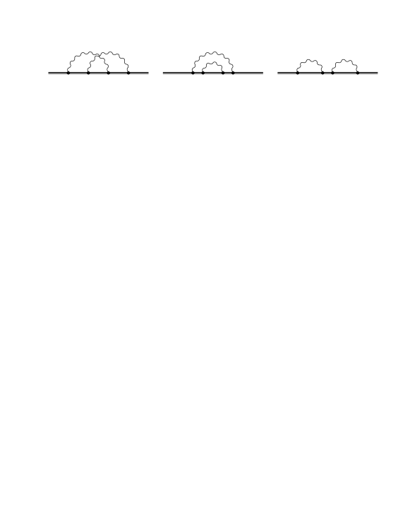
Figure 1: Pure two-loop self-energy diagrams (subset $i$ of the two-loop diagrams). The double line denotes the bound-electron propagator.

The form-factor contribution $E_{F}$ corresponds to an integration region where both photon momenta are of the order of the electron mass, but the electron momentum is of the order of $Z\,\alpha$. This part is a sum of two terms:

$$E_{F}=E_{F1}+E_{F2}\,.$$ (57)

The first term $E_{F1}$ comes from two-loop form factors, in the same way as the one-loop $E_{M1}$ [see Eq. (42)]. It contains additionally an iteration of the one-loop potential $\delta^{\rm(1)}V$ and the term proportional to $\kappa^{2}$ from Eq. (9):

$$E_{F1}=\langle\delta^{\rm(2)}V^{i}\rangle+2\,\left<\delta^{\rm(2)}V^{i}\,\frac{1}{(E-H)^{\prime}}\,H_{R}\right>+\frac{F^{\prime\rm(2)}_{1}(0)+2F^{\prime\rm(2)}_{2}(0)}{8}\,\langle\vec{\nabla}^{4}V+2\,{\rm i}\,\sigma^{ij}\,p^{i}\vec{\nabla}^{2}V\,p^{j}\rangle+F^{\prime\prime\rm(2)}_{1}(0)\,\langle\vec{\nabla}^{4}V\rangle$$ (58)

$$-\frac{F^{\rm(2)}_{2}(0)}{16}\,\left<\Bigl{\{}\vec{p}^{\,2},\vec{\nabla}^{2}V+2\,\sigma^{ij}\,\nabla^{i}V\,p^{j}\Bigr{\}}\right>+\frac{F^{\rm(2)}_{2}(0)+\left[F_{2}^{(1)}(0)\right]^{2}}{8}\,\langle(\vec{\nabla}V)^{2}\rangle+\left<\,\delta^{\rm(1)}V\,\frac{1}{(E-H)^{\prime}}\,\delta^{\rm(1)}V\,\right>.$$

The two-loop form factors are given in Eq. (108) below, and $\delta^{\rm(1)}V,\delta^{\rm(2)}V$ are the one- and two-loop components respectively of the potential given in Eq. (39). The explicit form of $\delta^{(2)}V^{i}$ can be found in Eq. (73) below.

$E_{F2}$ comes from the low-energy two-loop scattering amplitude and is the analog of the one-loop $E_{M2}$ in Eq. (44). The effective interaction is

$$\delta^{\rm(2)}H=\chi^{(2)}\,(\vec{\nabla}V)^{2}\,,$$ (59)

where $\chi^{(2)}$ is defined in Eq. (125b) below. It is assumed that vacuum polarization diagrams does not contribute in the current section to form factors as well as to $\chi$. The energy shift due to $\delta^{\rm(2)}H$ is

$$E_{F2}=\left<\delta^{\rm(2)}H\right>\,.$$ (60)

It is a remarkable fact that this two-loop scattering-amplitude contribution is infrared finite, in contrast to the corresponding one-loop result in Eq. (44).

For the two-loop problem, we redefine $E_{M}$ to be the contribution where one of the photon momenta is of the order of the electron mass, the second photon momentum is of order $(Z\,\alpha)^{2}$ and the electron momenta are of order $Z\,\alpha$. In the spirit of NRQED, the contribution coming from large photon momenta is accounted for by form factors. Therefore $E_{M}$ is given by the correction to Bethe logarithms coming from one-loop form factors. It is a sum of two parts

$$E_{M}=E_{M1}+E_{M2}\,.$$ (61)

The contribution $E_{M1}$ is similar to the one-loop term $E_{L1}$ with $H_{R}$ replaced by $\delta^{\rm(1)}V$:

$$E_{M1} = e^{2}\,\int\frac{d^{d}k}{(2\,\pi)^{d}\,2\,k}\,\frac{d-1}{d}\,\delta_{\delta^{\rm(1)}V}\,\left<\,\vec{p}\,\frac{1}{E-H-k}\,\vec{p}\,\right>\,.$$ (62)

We calculate it by splitting the integral in two parts $k<\Lambda$ and $k>\Lambda$ in analogy to the one-loop case,

$$E_{M1} = e^{2}\,\int_{0}^{\Lambda}\frac{d^{d}k}{(2\,\pi)^{d}\,2\,k}\,\frac{d-1}{d}\,\delta_{\delta^{\rm(1)}V}\,\left<\,\vec{p}\,\frac{1}{E-H-k}\,\vec{p}\,\right>$$ (63)

$$+\frac{\alpha}{\pi}\,\frac{\xi}{2}\,\left\{\left<[\vec{p},[\delta^{\rm(1)}V,\vec{p}]]\right>+2\,\left<\delta^{\rm(1)}V\,\frac{1}{(E-H)^{\prime}}\,\nabla^{2}V\right>\right\}\,,$$

where

$$\xi=\frac{1}{3\,\varepsilon}+\left\{\frac{5}{9}-\frac{2}{3}\,\ln[2\,(Z\,\alpha)^{2}]\right\}+\varepsilon\,\left\{\frac{28}{27}-\frac{2}{3}\,\zeta(2)+\frac{10}{9}\,\ln\left[{\textstyle{\frac{1}{2}}}\,(Z\,\alpha)^{-2}\right]+\frac{2}{3}\,\ln^{2}\left[{\textstyle{\frac{1}{2}}}\,(Z\,\alpha)^{-2}\right]\right\}\,.$$ (64)

We have not approached the limit $d=3$ in the first part, because $\delta^{\rm(1)}V$ contains $1/\varepsilon$. It will eventually cancel when combined with $E_{L}$, and only then one approaches this limit. $E_{M2}$ is similar to the one-loop $E_{L3}$ and comes from the $F_{2}(0)$-correction to the coupling with the radiation field,

$$H_{FW}=-\frac{e}{4}\,\sigma^{ij}\,B^{ij}\,[1+F_{2}(0)]-\frac{e}{8}\,[1+2\,F_{2}(0)][\nabla\cdot\vec{E}+\sigma^{ij}\,(E^{i}\,\pi^{j}+\pi^{j}\,E^{i})]\,,$$ (65)

which yields

$$\delta j^{i}=\frac{F_{2}^{(1)}(0)}{2}\,\sigma^{ik}\,(\vec{k}\cdot\vec{r}\,k^{k}+{\rm i}\,k\,p^{k}-\nabla^{k}V)\simeq-\frac{\alpha}{\pi}\,\frac{2\,d-3}{4\,(d-1)}\,\sigma^{ik}\,\nabla^{k}V\,.$$ (66)

The corresponding correction $E_{M2}$ is

$$E_{M2} = 2\,e^{2}\,\int\frac{d^{d}k}{(2\,\pi)^{d}\,2\,k}\,\left(\delta^{ij}-\frac{k^{i}\,k^{j}}{k^{2}}\right)\,\left<\delta j^{i}\frac{1}{E-H-k}\,p^{j}\right>$$ (67)

$$= -\frac{1}{2}\,\left(\frac{\alpha}{\pi}\right)^{2}\,\int_{0}^{\Lambda}dk\,k\,\left<\,\sigma^{ij}\,\nabla^{j}V\frac{1}{E-H-k}\,p^{i}\right>\,,$$

and this integral in $(Z\,\alpha)^{6}$ order does not depend on the cut-off in the limit $\lambda\rightarrow\infty$, when one drops the linear term in $\lambda$.

The low-energy part $E_{L}$, appropriately redefined for the two-loop problem, is a contribution from two low-energy photon momenta, $k_{i}\sim(Z\,\alpha)^{2}$. Its explicit expression is rather long:

$$E_{L}=\left[e^{2}\,\int\frac{d^{d}k_{1}}{(2\,\pi)^{d}\,2\,k_{1}}\,\frac{d-1}{d}\right]\,\left[e^{2}\,\int\frac{d^{d}k_{2}}{(2\,\pi)^{d}\,2\,k_{2}}\,\frac{d-1}{d}\right]\,P(k_{1},k_{2})\,,$$

$$P(k_{1},k_{2})=\left<p^{i}\,\frac{1}{E-(H+k_{1})}\,p^{j}\,\frac{1}{E-(H+k_{1}+k_{2})}\,p^{i}\,\frac{1}{E-(H+k_{2})}\,p^{j}\right>$$

$$\quad+\frac{1}{2}\,\left<p^{i}\,\frac{1}{E-(H+k_{1})}\,p^{j}\,\frac{1}{E-(H+k_{1}+k_{2})}\,p^{j}\,\frac{1}{E-(H+k_{1})}\,p^{i}\right>$$

$$\quad+\frac{1}{2}\,\left<p^{i}\,\frac{1}{E-(H+k_{2})}\,p^{j}\,\frac{1}{E-(H+k_{1}+k_{2})}\,p^{j}\,\frac{1}{E-(H+k_{2})}\,p^{i}\right>$$

$$\quad+\left<p^{i}\,\frac{1}{E-(H+k_{1})}\,p^{i}\,\frac{1}{(E-H)^{\prime}}\,p^{j}\,\frac{1}{E-(H+k_{2})}\,p^{j}\right>$$

$$\quad-\frac{1}{2}\,\left<p^{i}\,\frac{1}{E-(H+k_{1})}\,p^{i}\right>\,\left<p^{j}\,\frac{1}{[E-(H+k_{2})]^{2}}\,p^{j}\right>-\frac{1}{2}\,\left<p^{i}\,\frac{1}{E-(H+k_{2})}\,p^{i}\right>\,\left<p^{j}\,\frac{1}{[E-(H+k_{1})]^{2}}\,p^{j}\right>$$

$$\quad+\left<p^{i}\frac{1}{E-(H+k_{1})}\frac{1}{E-(H+k_{2})}p^{i}\right>-\frac{1}{k_{1}+k_{2}}\left<p^{i}\frac{1}{E-(H+k_{2})}p^{i}\right>-\frac{1}{k_{1}+k_{2}}\left<p^{i}\frac{1}{E-(H+k_{1})}p^{i}\right>.$$ (68)

We calculate $E_{L}$ by splitting both integrals in a way similar to the derivation presented in Pa2001 ,

$$E_{L} = \left(\frac{\alpha}{\pi}\right)^{2}\,\frac{(Z\,\alpha)^{6}}{n^{3}}\,b_{L}+e^{2}\,\int^{\Lambda}_{0}\,\frac{d^{d}k_{2}}{(2\,\pi)^{d}\,2\,k_{2}}\,\frac{d-1}{d}\,\frac{\alpha}{\pi}\,\frac{\xi}{2}\,\delta_{\nabla^{2}V}\,\left<\,\vec{p}\,\frac{1}{E-H-k}\,\vec{p}\,\right>$$ (69)

$$+\left[\frac{\alpha}{\pi}\,\frac{\xi}{2}\right]^{2}\,\left[\left<\vec{\nabla}^{2}V\,\frac{1}{(E-H)^{\prime}}\,\vec{\nabla}^{2}V\right>+\frac{1}{2}\,\left<\vec{\nabla}^{4}V\right>\right]\,.$$

Here, the two-loop Bethe logarithm $b_{L}$ is obtained as the finite part of the integral

$$\frac{(Z\,\alpha)^{6}}{n^{3}}\,b_{L}=\frac{4}{9}\,\int_{0}^{\Lambda_{1}}dk_{1}\,k_{1}\,\int_{0}^{\Lambda_{2}}dk_{2}\,k_{2}\,P(k_{1},k_{2})\,,$$ (70)

where it is assumed that the following limits are performed in order: first $d\rightarrow 3$, next $\lambda_{2}\rightarrow\infty$ and finally $\lambda_{1}\rightarrow\infty$ in the above. This definition of $b_{L}$ corresponds to the one in Refs. PaJe2003 ; Je2004b60 .

IV.2 General result for the pure two-loop self-energy

The pure two-loop self-energy contribution up to the order $\alpha^{2}\,(Z\,\alpha)^{6}$, denoted $\delta^{(2)}E^{i}$ (see Fig. 1), may now be obtained as the sum of $E_{F}+E_{M}+E_{L}$. With the partial results given in Eqs. (57), (61) and (IV.1), respectively, we obtain

$$\delta^{(2)}E^{i}=\left<\delta^{(2)}V^{i}\right>+\left(\frac{\alpha}{\pi}\right)^{2}\,\frac{(Z\,\alpha)^{6}}{n^{3}}\,\left[b_{L}+\left(\frac{10}{9}+\frac{4}{3}\ln\left[{\textstyle{\frac{1}{2}}}\,(Z\,\alpha)^{-2}\right]\right)\,N+\beta_{4}+\beta_{5}\right]+\left<V_{I}\frac{1}{(E-H)^{\prime}}\,V_{I}\right>$$

$$+2\,\left<\delta^{(2)}V^{i}\,\frac{1}{(E-H)^{\prime}}\,H_{R}\right>+\left(\frac{\alpha}{\pi}\right)^{2}\,\left[\frac{31}{256}+\frac{3}{16}\,\zeta(2)\,\ln(2)-\frac{5}{32}\,\zeta(2)-\frac{3}{64}\,\zeta(3)\right]\,\left<\Bigl{\{}p^{2},\vec{\nabla}^{2}V+2\,\sigma^{ij}\,\nabla^{i}V\,p^{j}\Bigr{\}}\right>$$

$$+\left(\frac{\alpha}{\pi}\right)^{2}\,\left[-\frac{559}{1152}+\frac{17}{8}\zeta(2)\,{\ln(2)}-\frac{41}{72}\,\zeta(2)-\frac{17}{32}\,\zeta(3)\right]\,\langle(\vec{\nabla}V)^{2}\rangle$$

$$+\left(\frac{\alpha}{\pi}\right)^{2}\,\left[-\frac{3295}{41472}+\frac{9}{10}\zeta(2)\,\ln(2)-\frac{4063}{14400}\zeta(2)-\frac{9}{40}\zeta(3)+\frac{5}{54}\ln\left[{\textstyle{\frac{1}{2}}}\,(Z\,\alpha)^{-2}\right]+\frac{1}{18}\ln^{2}\left[{\textstyle{\frac{1}{2}}}\,(Z\,\alpha)^{-2}\right]\right]\,\langle\vec{\nabla}^{4}V\rangle$$

$$+\left(\frac{\alpha}{\pi}\right)^{2}\,\left[-\frac{3059}{23040}-\frac{1}{5}\,\zeta(2)\,\ln(2)+\frac{1321}{5760}\,\zeta(2)+\frac{1}{20}\,\zeta(3)+\frac{1}{24}\,\ln\left[{\textstyle{\frac{1}{2}}}\,(Z\,\alpha)^{-2}\right]\right]\,\langle 2\,{\rm i}\,\sigma^{ij}\,p^{i}\,\vec{\nabla}^{2}V\,p^{j}\rangle.$$ (71)

Here, the first term $\langle\delta^{(2)}V^{i}\rangle$ is of lower-order [$\alpha^{2}(Z\alpha)^{4}$], and

$$V_{I} = \frac{\alpha}{\pi}\,\left[\frac{\vec{\nabla}^{2}V}{4}\,\left(\frac{10}{9}\,+\frac{4}{3}\ln\left[{\textstyle{\frac{1}{2}}}\,(Z\,\alpha)^{-2}\right]\right)+\frac{\sigma^{ij}}{4}\,\nabla^{i}\,V\,p^{j}\right]\,.$$ (72)

$$\delta^{(2)}V^{i} = \left(\frac{\alpha}{\pi}\right)^{2}\,\left\{\left[-\frac{163}{288}+\frac{9}{4}\,\zeta(2)\,\ln 2-\frac{85}{144}\,\zeta(2)-\frac{9}{16}\,\zeta(3)\right]\,\vec{\nabla}^{2}V\right.$$ (73)

$$\left.+\left[-\frac{31}{32}-\frac{3}{2}\,\zeta(2)\,\ln 2+\frac{5}{4}\,\zeta(2)+\frac{3}{8}\,\zeta(3)\right]\,\sigma^{ij}\,\nabla^{i}V\,p^{j}\right\}\,.$$

The various generalized Bethe logarithms that enter into Eq. (IV.2), are given as follows (with the implicit assumption that polynomial divergences as well as logarithmic ones for large $\lambda=\Lambda/(Z\,\alpha)^{2}$ are dropped)

$$\frac{(Z\,\alpha)^{6}}{n^{3}}\,N = \frac{2}{3}\,Z\,\alpha\,\int_{0}^{\Lambda}\,dk\,k\,\delta_{\pi\,\delta^{3}(r)}\left<\,\vec{p}\,\frac{1}{E-H-k}\,\vec{p}\,\right>\,,$$ (74a)

$$\frac{(Z\,\alpha)^{6}}{n^{3}}\,\beta_{4} = \frac{2}{3}\,\int_{0}^{\Lambda}dk\,k\,\delta_{(\sigma^{ij}\nabla^{i}\,V\,p^{j}/4)}\left<\,\vec{p}\,\frac{1}{E-H-k}\,\vec{p}\,\right>\,,$$ (74b)

$$\frac{(Z\,\alpha)^{6}}{n^{3}}\,\beta_{5} = \frac{2}{3}\,\int_{0}^{\Lambda}dk\,k\,\left<-\frac{3}{4}\,\sigma^{ij}\nabla^{j}V\frac{1}{E-H-k}\,p^{i}\right>\,,$$ (74c)

The $N$ term has previously been defined in Refs. Pa2001 ; PaJe2003 ; it is generated by a Dirac delta correction to the Bethe logarithm. All the explicit matrix element occurring in the formula (IV.2) can be calculated using standard techniques, for arbitrary hydrogenic states with nonvanishing angular momentum, and for the normalized difference (13) of $S$ states. The evaluation of the generalized Bethe logarithms $N$, $\beta_{4}$, and $\beta_{5}$ is more complicated (see Refs. Je2003jpa ; JeEtAl2003 ). The calculation of the two-loop Bethe logarithm $b_{L}$ for arbitrary excited hydrogenic states is a challenging numerical problem. So far results have been obtained only for excited $S$ states PaJe2003 ; Je2004b60 . The formula (IV.2) thus provides the basis for complete two-loop calculations in the order $\alpha^{2}\,(Z\,\alpha)^{6}$, and reduces the remaining part of the problem, for a general hydrogenic state, to a well-defined and in essence merely technical numerical calculations. In the following sections we discuss the evaluation of the formula (IV.2) for particular hydrogenic states for which the generalized Bethe logarithms can be inferred from previous calculations. These comprise the fine-structure difference of $D$ and $P$ states, and the normalized difference for $S$ states.

Table 2: Numerical values for the pure two-loop self-energy diagrams as shown in Fig. 1. The $B_{60}$-coefficients receive a superscript $i$.

$n$	$B^{i}_{60}(D_{5/2}-D_{3/2})$	$B^{i}_{60}(P_{3/2}-P_{1/2})$	$b_{L}(nS)$	$N(nS)$	$R(n)$	$B^{i}_{60}(nS)-B^{i}_{60}(1S)$
1	—	—	$-81.4(3)$	$17.855\,672\,03(1)$	—	—
2	—	$-0.361~{}196$	$-66.6(3)$	$12.032\,141\,58(1)$	$-0.671\,347$	$14.1(4)$
3	$-0.018~{}955$	$-0.410~{}149$	$-63.5(6)$	$10.449\,809(1)$	$-1.041\,532$	$16.9(7)$
4	$-0.022~{}253$	$-0.419~{}927$	$-61.8(8)$	$9.722\,413(1)$	$-1.254\,980$	$18.3(10)$
5	$-0.023~{}395$	$-0.420~{}828$	$-60.6(8)$	$9.304\,114(1)$	$-1.392\,573$	$19.4(11)$
6	$-0.023~{}826$	$-0.419~{}339$	$-59.8(8)$	$9.031\,832(1)$	$-1.488\,456$	$20.1(11)$

IV.3 Results for the fine-structure difference of $D$ states

For $D$ states, we use the general result (IV.2) and the fact that matrix elements involving a Dirac-delta function vanish. Thus, logarithmic terms for $D$ levels vanish, $B^{i}_{61}(D_{3/2})=B^{i}_{61}(D_{5/2})=0$. The absence of logarithmic terms even holds for the sum of all two-loop diagrams (not only for the subset $i$), and even for arbitrary states with orbital angular momentum $l>2$. This result generalizes the well-known fact that the double-logarithmic contribution $B_{62}$ vanishes for states with $l\geq 2$ Ka1996 ; JeNa2002 . For the fine-structure difference of $B^{i}_{60}$, we use the result in Eq. (IV.2) and the matrix elements in Eq. (48), to obtain

$$B^{i}_{60}(D_{5/2}-D_{3/2})=-\frac{38497}{403200}-\frac{133}{640\,n}+\frac{895}{1344\,n^{2}}+\left(-\frac{3817}{25200}-\frac{13}{40\,n}+\frac{29}{28\,n^{2}}\right)\,\zeta(2)\,\ln(2)$$

$$+\left(\frac{3817}{30240}+\frac{13}{48\,n}-\frac{145}{168\,n^{2}}\right)\,\zeta(2)+\left(\frac{3817}{100800}+\frac{13}{160\,n}-\frac{29}{112\,n^{2}}\right)\,\zeta(3)+\beta_{4}(D_{5/2}-D_{3/2})+\beta_{5}(D_{5/2}-D_{3/2})\,.$$ (75)

Numerical data for $B_{60}(D_{5/2}-D_{3/2})$ can be found in Tab. IV.2. The unknown two-loop Bethe logarithm $b_{L}(nD)$ does not contribute to the fine-structure difference of $D$ states.

IV.4 Results for the fine-structure difference of $P$ states

We again use the fact that the unknown two-loop Bethe logarithm $b_{L}$ does not contribute to the fine-structure difference of $P$ states. With the help of the general result in Eq. (IV.2) and the matrix elements in Eq. (50), we obtain

$$B_{61}(P_{3/2}-P_{1/2})=-\frac{1}{3}\,\left(1-\frac{1}{n^{2}}\right)$$ (76)

in agreement with the literature JePa2002 and

$$B^{i}_{60}(P_{3/2}-P_{1/2})=-\frac{217}{1280}-\frac{151}{128\,n}+\frac{325}{288\,n^{2}}+\left(\frac{1}{3}-\frac{1}{3\,n^{2}}\right)\,\ln(2)+\left(-\frac{103}{240}-\frac{15}{8\,n}+\frac{37}{20\,n^{2}}\right)\,\zeta(2)\,\ln(2)$$

$$+\left(-\frac{23}{160}+\frac{25}{16\,n}-\frac{749}{720\,n^{2}}\right)\,\zeta(2)+\left(\frac{103}{960}+\frac{15}{32\,n}-\frac{37}{80\,n^{2}}\right)\,\zeta(3)+\beta_{4}(P_{3/2}-P_{1/2})+\beta_{5}(P_{3/2}-P_{1/2})\,.$$ (77)

Numerical values of the relevant quantities for $n=2,\dots,6$ can be found in Tab. IV.2. They are in full agreement with results previously obtained in JePa2002 . The generalized Bethe logarithms $\beta_{4}$ and $\beta_{5}$ in these expressions are equivalent to the quantities $\Delta_{\mathrm{fs}}{{\ell}}_{4}(n)$ and $\Delta_{\mathrm{fs}}{{\ell}}_{5}(n)$ as defined in Ref. JePa2002 . In the context of the current investigation, the numerical values of $\Delta_{\mathrm{fs}}{{\ell}}_{4}(n)$ and $\Delta_{\mathrm{fs}}{{\ell}}_{5}(n)$ were reevaluated with improved accuracy as compared to Ref. JeKePa2002 and the data in Tab. IV.2 are consistent with them.

IV.5 Results for the normalized difference of $S$ states

We evaluate the general formula given in Eq. (IV.2) for the normalized difference of $S$ states, using the matrix elements given in Eq. (52). In the result, we identify terms with the square of the logarithm $\ln[(Z\,\alpha)^{-2}]$ ($B^{i}_{62}$ coefficient), and with single logarithm ($B^{i}_{61}$ coefficient), and the nonlogarithmic term $B^{i}_{60}$. The results discussed here probably are the phenomenologically most important ones reported in this paper, because of the high accuracy of two-photon spectroscopic experiments which involve $S$–$S$ transitions.

For the double-logarithmic term, we recover the following known result (see Refs. Pa2001 ; Je2003plb ),

$$B^{i}_{62}(nS)-B^{i}_{62}(1S) = \frac{16}{9}\left(\frac{3}{4}+\frac{1}{4n^{2}}-\frac{1}{n}+\gamma-\ln(n)\!+\!\Psi(n)\right)\,.$$ (78)

Here $\Psi$ denotes the logarithmic derivative of the gamma function, and $\gamma=0.577216\dots$ is Euler’s constant. The result for $B_{61}$, restricted to the two-loop diagrams in Fig. 1, reads Pa2001 ; Je2003plb

$$B^{i}_{61}(nS)-B^{i}_{61}(1S)=\frac{4}{3}\,\left[N(nS)-N(1S)\right]+\left(\frac{80}{27}-\frac{32}{9}\,\ln 2\right)\,\left(\frac{3}{4}-\frac{1}{n}+\frac{1}{4n^{2}}+\gamma-\ln(n)+\Psi(n)\right)\,.$$ (79)

This result is recovered here from Eq. (IV.2), using the matrix elements in Eq. (52). Moreover, we obtain the complete $n$-dependence of the nonlogarithmic term $B^{i}_{60}$:

$$B^{i}_{60}(nS)-B^{i}_{60}(1S)=b_{L}(nS)-b_{L}(1S)+\left(\frac{10}{9}-\frac{4}{3}\,\ln(2)\right)\,[N(nS)-N(1S)]$$

$$+\frac{10529}{5184}-\frac{14099}{2592\,n}+\frac{17699}{5184\,n^{2}}+\left(\frac{4}{3}-\frac{16}{9\,n}+\frac{4}{9\,n^{2}}\right)\,\ln^{2}(2)+\left(-\frac{20}{9}+\frac{80}{27\,n}-\frac{20}{27\,n^{2}}\right)\,\ln(2)$$

$$+\left(-\frac{53}{15}+\frac{35}{2\,n}-\frac{149}{30\,n^{2}}\right)\,\zeta(2)\,\ln(2)+\left(\frac{1357}{2700}-\frac{167}{36\,n}+\frac{2792}{675\,n^{2}}\right)\,\zeta(2)+\left(\frac{53}{60}-\frac{35}{8\,n}+\frac{419}{120\,n^{2}}\right)\,\zeta(3)$$

$$+\left(-\frac{497}{1296}+\frac{16}{9}\ln^{2}(2)-\frac{80}{27}\ln(2)+8\,\zeta(2)\ln(2)-\frac{79}{36}\zeta(2)-2\,\zeta(3)\right)\,\left[\gamma+\Psi(n)-\ln(n)\right]\,.$$ (80)

The generalized Bethe logarithms $\beta_{4}$ and $\beta_{5}$, which make an occurrence in Eq. (IV.2) but are not present in Eq. (IV.5), vanish for $S$ states. The result (IV.5) can also be written as

$$B^{i}_{60}(nS)-B^{i}_{60}(1S)=b_{L}(nS)-b_{L}(1S)+R(n)\,,$$ (81)

which provides a definition of the remainder $R(n)$. Numerical values for $b_{L}(nS)$, $N(nS)$, $R(n)$ and the normalized $S$-state difference $B^{i}_{60}(nS)-B^{i}_{60}(1S)$ are given in Table IV.2, and we have the opportunity to correct a calculational error for $N(2S)$ whose value had previously been given as $12.032209$ in Je2003jpa .

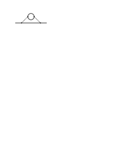
Figure 2: Feynman diagram with a vacuum-polarization loop in the self-energy virtual photon line (this single diagram forms subset $ii$ in the convention adopted in this paper).

V FERMION LOOP IN THE SELF-ENERGY PHOTON LINE

We here calculate the mixed self-energy vacuum-polarization diagram in Fig. 2. The result can be easily inferred from the terms in square brackets in Eqs. (59), (108), and (125), and reads

$$\delta^{(2)}E^{ii}=\left<\delta^{(2)}V^{ii}\right>+2\,\left<\delta^{(2)}V^{ii}\,\frac{1}{(E-H)^{\prime}}\,H_{R}\right>+\left(\frac{\alpha}{\pi}\right)^{2}\,\left[-\frac{119}{576}+\frac{1}{8}\,\zeta(2)\right]\,\left<\Bigl{\{}p^{2},\vec{\nabla}^{2}V+2\,\sigma^{ij}\,\nabla^{i}V\,p^{j}\Bigr{\}}\right>$$

$$+\left(\frac{\alpha}{\pi}\right)^{2}\,\left\{\left[\frac{119}{288}-\frac{1}{4}\,\zeta(2)\right]\langle(\vec{\nabla}V)^{2}\rangle+\left[-\frac{4511}{51840}+\frac{65}{1152}\,\zeta(2)\right]\langle\vec{\nabla}^{4}V\rangle+\left[\frac{2633}{10368}-\frac{175}{1152}\,\zeta(2)\right]\,\langle 2\,{\rm i}\,\sigma^{ij}\,p^{i}\,\vec{\nabla}^{2}V\,p^{j}\rangle\right\},$$ (82)

where

$$\delta^{(2)}V^{ii}=\left(\frac{\alpha}{\pi}\right)^{2}\,\left\{\left[-\frac{7}{324}+\frac{5}{144}\,\zeta(2)\right]\,\vec{\nabla}^{2}V+\left[\frac{119}{72}-\zeta(2)\right]\,\sigma^{ij}\,\nabla^{i}V\,p^{j}\right\}\,.$$ (83)

is a radiative potential in the sense of Eq. (39), but includes here only the vacuum polarization part of form factors. We observe the absence of $\ln(Z\,\alpha)$ terms.

Table 3: Values of the fine-structure for $D$ and $P$ states and normalized difference of $S$ states coming from from fermion loop diagrams in Fig. 2.

$n$	$B^{ii}_{60}(D_{5/2}-D_{3/2})$	$B^{ii}_{60}(P_{3/2}-P_{1/2})$	$B^{ii}_{60}(nS)-B^{ii}_{60}(1S)$
2	—	$-0.013\,435$	$0.109\,999$
3	$0.000\,757$	$-0.017\,089$	$0.114\,502$
4	$0.000\,878$	$-0.018\,613$	$0.110\,743$
5	$0.000\,915$	$-0.019\,431$	$0.106\,566$
6	$0.000\,925$	$-0.019\,935$	$0.102\,982$

Numerical values for $S$, $P$, and $D$ states can now be obtained using matrix elements in Eqs. (48), (50) and (52). For the fine-structure intervals, we obtain

$$B^{ii}_{60}(D_{5/2}-D_{3/2})= \frac{64889}{388800}+\frac{1547}{4320\,n}-\frac{493}{432\,n^{2}}+\left(-\frac{3817}{37800}-\frac{13}{60\,n}+\frac{29}{42\,n^{2}}\right)\,\zeta(2)\,,$$ (84)

$$B^{ii}_{60}(P_{3/2}-P_{1/2})= \frac{5293}{25920}+\frac{595}{288\,n}-\frac{2867}{1620\,n^{2}}+\left(-\frac{11}{80}-\frac{5}{4\,n}+\frac{781}{720\,n^{2}}\right)\,\zeta(2)\,.$$ (85)

Considering $S$ states, as is evident from Eq. (V), using the matrix elements in Eq. (52), the normalized difference of $B^{ii}_{61}$ vanishes, $B^{ii}_{61}(nS)-B^{ii}_{61}(1S)=0$, and this result is in agreement with the literature. For the normalized $n$-dependence of $B^{ii}_{60}$, we obtain the following result,

$$B^{ii}_{60}(nS)-B^{ii}_{60}(1S)= -\frac{21319}{6480}+\frac{1015}{648\,n}+\frac{1241}{720\,n^{2}}+\left(\frac{301}{144}-\frac{31}{36\,n}-\frac{59}{48\,n^{2}}\right)\,\zeta(2)$$

$$+\left[\frac{1099}{324}-\frac{77}{36}\,\zeta(2)\right]\,\left[\gamma+\Psi(n)-\ln(n)\right]\,.$$ (86)

Numerical values are presented in Tab. V.

VI COMBINED SELF-ENERGY WITH A FERMION LOOP IN THE COULOMB PHOTON LINE

The Feynman diagrams in Fig. 3 represent the modification of a leading one-loop self-energy correction by a perturbing Uehling potential $V_{U}=-\frac{4}{15}\,\alpha\,(Z\alpha)\,\delta^{d}(r)=-\frac{\alpha}{15\,\pi}\,\vec{\nabla}^{2}V$. One can easily obtain the result from $E_{L0}+E_{M0}$ in Eqs. (19) and (40), by replacing the Coulomb potential $V$ by $V+V_{U}$, and expanding all matrix elements in $V_{U}$, up to the linear terms. The result is

$$\delta^{(2)}E^{iii}= -\frac{4}{15}\,\left(\frac{\alpha}{\pi}\right)^{2}\,\frac{(Z\,\alpha)^{6}}{n^{3}}\,N-\frac{1}{15}\,\left(\frac{\alpha}{\pi}\right)^{2}\,\left[\frac{5}{9}+\frac{2}{3}\,\ln\left[{\textstyle{\frac{1}{2}}}\,(Z\alpha)^{-2}\right]\right]\,\left<\vec{\nabla}^{2}V\,\left(\frac{1}{E-H}\right)^{\prime}\,\vec{\nabla}^{2}V\right>$$

$$-\frac{1}{120}\,\left(\frac{\alpha}{\pi}\right)^{2}\,\langle 2\,{\rm i}\,\sigma^{ij}\,p^{i}\,\vec{\nabla}^{2}V\,p^{j}\rangle-\left(\frac{\alpha}{\pi}\right)^{2}\,\left[\frac{1}{54}+\frac{1}{45}\,\ln\left[{\textstyle{\frac{1}{2}}}\,(Z\alpha)^{-2}\right]\right]\,\left<\vec{\nabla}^{4}V\right>\,.$$ (87)

Here, $N$ is a correction to the Bethe logarithm as defined in Eq. (74a). All matrix elements in this result vanish for $D$-states and for states with higher angular momenta. The absence of both logarithmic as well as nonlogarithmic terms holds from subset $iii$ holds for arbitrary states with orbital angular momentum $l>2$. For $P$ states, we obtain the fine-structure difference $B^{iii}_{61}(nP_{3/2})-B^{iii}_{61}(nP_{1/2})=0$, in agreement with the literature. For the nonlogarithmic term, we obtain

$$B^{iii}_{60}(nP_{3/2})-B^{iii}_{60}(nP_{1/2})=\frac{1}{15}\,\left(1-\frac{1}{n^{2}}\right)\,.$$ (88)

As a last example, we consider the $S$-state normalized difference defined in Eq. (13). using matrix elements given in (52). For the double-logarithmic term, we recover the known result $B^{iii}_{62}(nS)=0$ (see Refs. Pa2001 ; Je2003plb ). The result for $B^{iii}_{61}$ reads Pa2001 ; Je2003plb

$$B^{iii}_{61}(nS)-B^{iii}_{61}(1S)$$ (89)

$$= -\frac{32}{45}\left(\frac{3}{4}+\frac{1}{4n^{2}}-\frac{1}{n}+\gamma+\Psi(n)-\ln(n)\right)\,.$$

This result is recovered here from Eq. (VI). As a new result, we obtain the complete $n$-dependence of the nonlogarithmic term $B^{iii}_{60}$:

$$B^{iii}_{60}(nS)-B^{iii}_{60}(1S)=-\frac{4}{15}\,\left[N(nS)-N(1S)\right]$$

$$-\frac{4}{9}+\frac{16}{27n}-\frac{4}{27n^{2}}+\left(\frac{8}{15}-\frac{32}{45n}+\frac{8}{45n^{2}}\right)\ln(2)$$

$$+\left(-\frac{16}{27}+\frac{32}{45}\,\ln(2)\right)\,\left[\gamma+\Psi(n)-\ln(n)\right]\,.$$ (90)

Using this formula, it is then possible to infer the values of $B^{iii}_{60}(nS)-B^{iii}_{60}(1S)$ as given in Tab. VI.

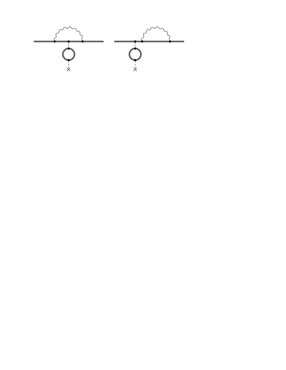
Figure 3: Two-loop diagrams (subset $iii$) generated by a fermion loop in the Coulomb exchange of a one-loop self-energy.

Table 4: Values of the difference $B^{iii}_{60}(nS)-B^{iii}_{60}(1S)$ for the diagrams in subset $iii$.

$n$	$B^{iii}_{60}(nS)-B^{iii}_{60}(1S)$
2	$1.491\,199$
3	$1.890\,577$
4	$2.072\,903$
5	$2.177\,348$
6	$2.245\,177$

VII PURE TWO-LOOP VACUUM POLARIZATION

We investigate the subset of Feynman diagrams in Fig. 4. The vacuum polarization correction to the Coulomb potential is

$$-\frac{4\pi\,Z\,\alpha}{\vec{q}^{\,2}}\to-\frac{4\pi\,Z\,\alpha}{\vec{q}^{\,2}}\,\frac{1}{\left(1+{\bar{\omega}}(-\vec{q}^{\,2})\right)}$$

$$=-\frac{4\pi\,Z\,\alpha}{\vec{q}^{\,2}}\,\left[1-{\bar{\omega}}(-\vec{q}^{\,2})+{\bar{\omega}}(-\vec{q}^{\,2})^{2}+\ldots\right]\,,$$ (91)

where the one- and two-loop parts read Sc1970 ; BaRe1973 as follows,

$${\bar{\omega}}(-\vec{q}^{\,2})= {\bar{\omega}}^{(1)}(-\vec{q}^{\,2})+{\bar{\omega}}^{(2)}(-\vec{q}^{\,2})+\,\ldots,$$

$${\bar{\omega}}^{(1)}(-\vec{q}^{\,2})= \left(\frac{\alpha}{\pi}\right)\,(-\vec{q}^{\,2})\,\left(\frac{1}{15}-\frac{\vec{q}^{\,2}}{140}+\ldots\right)\,,$$ (92)

$${\bar{\omega}}^{(2)}(-\vec{q}^{\,2})= \left(\frac{\alpha}{\pi}\right)^{2}\,(-\vec{q}^{\,2})\left(\frac{41}{162}-\frac{449\,\vec{q}^{\,2}}{10800}+\ldots\right)\,.$$ (93)

In the integral representation for ${\bar{\omega}}^{(2)}$ given in Eqs. (15) and (16) of Ref. Pa1993 , one should make the replacement $\ln\left(\frac{1+\delta}{1-\delta}\right)\to\ln\left(\frac{1+\delta}{1-\delta}\right)\,\ln\left(\frac{1+\delta}{2}\right)$ in order to correct for a typographical error in an intermediate step of this calculation. In the coordinate space, the correction becomes

$$V_{\rm vp}=\left[-{\bar{\omega}}(\nabla^{2})+{\bar{\omega}}(\nabla^{2})^{2}+\ldots\right]V\,.$$ (94)

The contributions to the energy involves the first and second order matrix element together with relativistic corrections,

$$\delta E= \left\langle V_{\rm vp}\right\rangle+\left\langle V_{\rm vp}\,\frac{1}{(E-H)^{\prime}}\,V_{\rm vp}\right\rangle$$

$$+2\,\left\langle V_{\rm vp}\,\frac{1}{(E-H)^{\prime}}\,H_{R}\right\rangle$$

$$+\frac{1}{8}\,\left\langle\nabla^{2}(V_{\rm vp})+2\,\sigma^{ij}\,\nabla^{i}(V_{\rm vp})\,p^{j}\right\rangle\,.$$ (95)

The two-loop part of this expression reads

$$\delta^{(2)}E^{iv}= -\frac{41}{162}\,\left(\frac{\alpha}{\pi}\right)^{2}\,\left<\vec{\nabla}^{2}V\right>$$

$$-\frac{953}{16200}\,\left(\frac{\alpha}{\pi}\right)^{2}\,\left<\vec{\nabla}^{2}V\,\frac{1}{(E-H)^{\prime}}\,\vec{\nabla}^{2}V\right>$$

$$+\frac{41}{648}\,\left(\frac{\alpha}{\pi}\right)^{2}\,\left<\vec{\nabla}^{2}V\,\frac{1}{(E-H)^{\prime}}\,\vec{p}^{4}\right>$$

$$-\frac{41}{1296}\,\left(\frac{\alpha}{\pi}\right)^{2}\,\langle 2\,{\rm i}\,\sigma^{ij}\,p^{i}\,\vec{\nabla}^{2}V\,p^{j}\rangle$$

$$-\frac{557}{8100}\,\left(\frac{\alpha}{\pi}\right)^{2}\,\langle\vec{\nabla}^{4}V\rangle$$ (96)

The first term in this result corresponds to the $\alpha^{2}\,(Z\,\alpha)^{4}$ term in Eq. (IV.1). The remaining terms give the $B^{iv}_{60}$ coefficient.

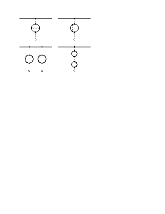
Figure 4: The remaining two-loop diagrams (subset $iv$) involve at least one closed fermion loop in the Coulomb photon exchange between electron and nucleus, and no self-energy photons.

Table 5: Values of the difference $B^{iv}_{60}(nS)-B^{iv}_{60}(1S)$ for the diagrams in subset $iv$.

$n$	$B^{iv}_{60}(nS)-B^{iv}_{60}(1S)$
2	$-0.611\,365$
3	$-0.603\,468$
4	$-0.560\,004$
5	$-0.521\,300$
6	$-0.490\,240$

We first notice the complete absence of logarithmic terms in the result (VII). All matrix elements in (VII) vanish for $D$-states and for states with higher angular momenta, in the order of $\alpha^{2}\,(Z\alpha)^{6}$. The fine-structure difference of the nonlogarithmic term for $P$ states is as follows,

$$B^{iv}_{60}(nP_{3/2})-B^{iv}_{60}(nP_{1/2})=\frac{41}{162}\,\left(1-\frac{1}{n^{2}}\right)\,.$$ (97)

The $n$-dependence of the nonlogarithmic term $B^{iv}_{60}$ is as follows,

$$B^{iv}_{60}(nS)-B^{iv}_{60}(1S)=-\frac{1817}{2025}-\frac{2194}{2025n}+\frac{1337}{675n^{2}}$$

$$+\frac{2194}{2025}\,\left[\gamma+\Psi(n)-\ln(n)\right]\,.$$ (98)

This completes our investigation of the subset $iv$.

VIII TOTAL RESULT FOR ALL TWO–LOOP DIAGRAMS

The two-loop subsets $i$—$iv$ (see Figs. 1—4) have been considered in Secs. IV—VII. We are now in the position to add the results given in Eqs. (IV.2), (V), (VI) and (VII), and to present a general expression for the complete two-loop correction to the Lamb shift, including the vacuum-polarization terms, valid for general hydrogenic bound states with nonvanishing angular momenta, and for the normalized difference of $S$ states. This general result reads

$$\delta^{(2)}E=\delta^{(2)}E^{i}+\delta^{(2)}E^{ii}+\delta^{(2)}E^{iii}+\delta^{(2)}E^{iv}$$

$$=\left(\frac{\alpha}{\pi}\right)^{2}\frac{(Z\alpha)^{4}}{n^{3}}\,\left\{B_{40}+(Z\alpha)^{2}\,\left[B_{62}\ln^{2}[(Z\alpha)^{-2}]+B_{61}\ln[(Z\alpha)^{-2}]+B_{60}\right]\right\}$$

$$=\left(\frac{\alpha}{\pi}\right)^{2}\,\left[-\frac{2179}{2592}+\frac{9}{4}\,\zeta(2)\,\ln 2-\frac{5}{9}\,\zeta(2)-\frac{9}{16}\,\zeta(3)\right]\,\left<\vec{\nabla}^{2}V\right>+\left[\frac{197}{288}-\frac{3}{2}\,\zeta(2)\,\ln 2+\frac{1}{4}\,\zeta(2)+\frac{3}{8}\,\zeta(3)\right]\,\left<\sigma^{ij}\,\nabla^{i}V\,p^{j}\right>$$

$$\quad+\left(\frac{\alpha}{\pi}\right)^{2}\frac{(Z\alpha)^{6}}{n^{3}}\,\left\{b_{L}+\beta_{4}+\beta_{5}+\left[\frac{38}{45}+\frac{4}{3}{\ln\left[{\textstyle{\frac{1}{2}}}(Z\alpha)^{-2}\right]}{}\right]\,N\right\}$$

$$\quad+\left(\frac{\alpha}{\pi}\right)^{2}\left[-\frac{42923}{259200}+\frac{9}{16}\zeta(2)\ln(2)-\frac{5\zeta(2)}{36}-\frac{9\zeta(3)}{64}+\frac{19}{135}{\ln\left[{\textstyle{\frac{1}{2}}}(Z\alpha)^{-2}\right]}+\frac{1}{9}{\ln\left[{\textstyle{\frac{1}{2}}}(Z\alpha)^{-2}\right]}\right]\left<\vec{\nabla}^{2}V\frac{1}{(E-H)^{\prime}}\vec{\nabla}^{2}V\right>$$

$$\quad+\left(\frac{\alpha}{\pi}\right)^{2}\,\left[\frac{2179}{10368}-\frac{9}{16}\,\zeta(2)\,\ln(2)+\frac{5}{36}\,\zeta(2)+\frac{9}{64}\,\zeta(3)\right]\,\left<\vec{\nabla}^{2}V\,\frac{1}{(E-H)^{\prime}}\,\vec{p}^{\,4}\right>$$

$$\quad+\left(\frac{\alpha}{\pi}\right)^{2}\,\left[-\frac{197}{1152}+\frac{3}{8}\,\zeta(2)\,\ln(2)-\frac{1}{16}\,\zeta(2)-\frac{3}{32}\,\zeta(3)\right]\,\left<\vec{p}^{\,4}\,\frac{1}{(E-H)^{\prime}}\,\sigma^{ij}\,\nabla^{i}V\,p^{j}\right>$$

$$\quad+\left(\frac{\alpha}{\pi}\right)^{2}\,\left[\frac{233}{576}-\frac{3}{4}\,\zeta(2)\,\ln(2)+\frac{1}{8}\,\zeta(2)+\frac{3}{16}\,\zeta(3)\right]\,\left<\sigma^{ij}\,\nabla^{i}V\,p^{j}\,\frac{1}{(E-H)^{\prime}}\,\sigma^{ij}\,\nabla^{i}V\,p^{j}\right>$$

$$\quad+\left(\frac{\alpha}{\pi}\right)^{2}\,\left[-\frac{197}{2304}+\frac{3}{16}\,\zeta(2)\,\ln(2)-\frac{1}{32}\,\zeta(2)-\frac{3}{64}\,\zeta(3)\right]\,\left<\left\{\vec{p}^{\,2},\vec{\nabla}^{2}V+2\,\sigma^{ij}\,\nabla^{i}V\,p^{j}\right\}\right>$$

$$\quad+\left(\frac{\alpha}{\pi}\right)^{2}\,\left[-\frac{83}{1152}+\frac{17}{8}\zeta(2)\,{\ln(2)}-\frac{59}{72}\,\zeta(2)-\frac{17}{32}\,\zeta(3)\right]\,\left<\left(\vec{\nabla}V\right)^{2}\right>$$

$$\quad+\left(\frac{\alpha}{\pi}\right)^{2}\,\left[-\frac{87697}{345600}+\frac{9}{10}\zeta(2)\,\ln(2)-\frac{2167}{9600}\zeta(2)-\frac{9}{40}\zeta(3)+\frac{19}{270}{\ln\left[{\textstyle{\frac{1}{2}}}(Z\alpha)^{-2}\right]}+\frac{1}{18}{\ln\left[{\textstyle{\frac{1}{2}}}(Z\alpha)^{-2}\right]}\right]\,\left<\vec{\nabla}^{4}V\right>$$

$$\quad+\left(\frac{\alpha}{\pi}\right)^{2}\,\left[-\frac{16841}{207360}-\frac{1}{5}\,\zeta(2)\,\ln(2)+\frac{223}{2880}\,\zeta(2)+\frac{1}{20}\,\zeta(3)+\frac{1}{24}\,{\ln\left[{\textstyle{\frac{1}{2}}}(Z\alpha)^{-2}\right]}\right]\,\left<2\,{\rm i}\,\sigma^{ij}\,p^{i}\,\vec{\nabla}^{2}V\,p^{j}\right>\,.$$ (99)

The third line in the above equation corresponds to the lower-order $\alpha^{2}(Z\alpha)^{4}$ contribution ($B_{40}$ coefficient). We now turn to the evaluation of this expression for $S$ states. The sum of the contributions in Eqs. (IV.5), (V), (VI) and (VII) corresponds to the sum of all the matrix elements in Eq. (VIII), evaluated for the normalized difference of $S$ states. The logarithmic terms Pa2001 have already been verified for the normalized difference. The $n$-dependence of the total nonlogarithmic term may be expressed as

$$B_{60}(nS)-B_{60}(1S)=b_{L}(nS)-b_{L}(1S)+A(n),$$ (100)

where $A(n)$ is an additional contribution beyond the $n$-dependence of the two-loop Bethe logarithm, defined in analogy to Eq. (81). The result for $A$ is

$$A(n)=\left(\frac{38}{45}-\frac{4}{3}\,\ln(2)\right)\,[N(nS)-N(1S)]-\frac{337043}{129600}-\frac{94261}{21600\,n}+\frac{902609}{129600\,n^{2}}+\left(\frac{4}{3}-\frac{16}{9\,n}+\frac{4}{9\,n^{2}}\right)\,\ln^{2}(2)$$ (101)

$$+\left(-\frac{76}{45}+\frac{304}{135\,n}-\frac{76}{135\,n^{2}}\right)\,\ln(2)+\left(-\frac{53}{15}+\frac{35}{2\,n}-\frac{419}{30\,n^{2}}\right)\,\zeta(2)\,\ln(2)+\left(\frac{28003}{10800}-\frac{11}{2\,n}+\frac{31397}{10800\,n^{2}}\right)\,\zeta(2)$$

$$+\left(\frac{53}{60}-\frac{35}{8n}+\frac{419}{120n^{2}}\right)\,\zeta(3)+\left(\frac{37793}{10800}+\frac{16}{9}\ln^{2}(2)-\frac{304}{135}\ln(2)+8\zeta(2)\ln(2)-\frac{13}{3}\zeta(2)-2\zeta(3)\right)\left[\gamma+\Psi(n)-\ln(n)\right]\,.$$

Numerically, $A(n)$ is found to be much smaller than $b_{L}(nS)-b_{L}(1S)$, as shown in Table VIII. This implies that the numerically most important contribution to $B_{60}(nS)-B_{60}(1S)$ is exclusively due to the two-loop Bethe logarithm. The theoretical uncertainty of $B_{60}(nS)-B_{60}(1S)$, for higher excited $nS$ states, is caused entirely by the numerical uncertainty of the two-loop Bethe logarithm $b_{L}(nS)$, with explicitly data for higher excited states taken from Ref. Je2004b60 .

Table 6: Total values of the difference $B_{60}(nS)-B_{60}(1S)$ coming from all diagrams.

$n$	$A(n)$	$B_{60}(nS)-B_{60}(1S)$
2	$0.318~{}486$	$15.1(4)$
3	$0.360~{}079$	$18.3(7)$
4	$0.368~{}661$	$20.0(10)$
5	$0.370~{}042$	$21.2(11)$
6	$0.369~{}462$	$22.0(11)$

For the fine-structure difference of $D$ states, the total two-loop results is obtained by evaluating the general result in Eq. (VIII) on $D$ states, or alternatively by adding just the contributions from subsets $i$ and $ii$ [see Eqs. (IV.3) and (84)], because the subsets $iii$ and $iv$ do not contribute to the $D$ fine structure. For the $P$-state fine structure, the sum of the results in Eqs. (IV.4), (85), (88), and (97) gives the complete result, including the nonlogarithmic term $B_{60}$. It has already been stressed that in order to determine the absolute value of $B_{60}$ for $P$ and $D$ states, an evaluation of the Bethe logarithm $b_{L}$ for these states would be required, and its knowledge is currently restricted to $S$ states.

Despite this, we may evaluate general logarithmic terms for $P$ and $D$ states. For $D$ states and states with higher angular momenta, a direct evaluation of Eq. (VIII) immediately reveals that the logarithmic terms vanish,

$$B_{62}(nD)=B_{61}(nD)=0\,.$$ (102)

The same holds for any hydrogenic states with orbital angular momentum $l\geq 2$. For $P$ states, an evaluation of (VIII) confirm that

$$B_{62}(nP)=\frac{4}{27}\frac{n^{2}-1}{n^{2}}.$$ (103)

Furthermore, the logarithmic terms are

$$B_{61}(nP_{1/2})= \frac{4}{3}\,N(nP)+\frac{n^{2}-1}{n^{2}}\left(\frac{166}{405}-\frac{8}{27}\,\ln 2\right)\,,$$ (104)

$$B_{61}(nP_{3/2})= \frac{4}{3}\,N(nP)+\frac{n^{2}-1}{n^{2}}\left(\frac{31}{405}-\frac{8}{27}\,\ln 2\right)\,.$$ (105)

Numerical values for $N(nP)$ can be found in Eq. (17) of Ref. Je2003jpa .

IX SUMMARY

We have presented a unified approach to the one- and two-loop electron bound-state self-energy correction in hydrogenlike atoms, including terms of order $\alpha\,(Z\,\alpha)^{6}$ and $\alpha^{2}\,(Z\,\alpha)^{6}$, respectively. We consider states with nonvanishing orbital angular momentum and the normalized difference of $S$ states. The general analytic structure of the one- and two-loop corrections is given in Eqs. (14) and (IV.1), respectively. The general result for the one-loop correction is given in Eq. (46). We evaluate our formulas for specific families of hydrogenic states in Secs. III.5, III.6, and III.7 (one-loop case). All one-loop results are in agreement with those previously reported in the literature. In addition, we obtain results for the nonlogarithmic terms ($A_{60}$ coefficients), for higher excited $S$ states, as listed in Tab. 1.

For clarity, we separate the two-loop calculation into four different subsets $i$, $ii$, $iii$ and $iv$ consisting of separately gauge-invariant diagrams (see Secs. IV—VII and Figs. 1—4). A general formula for the “pure” two-loop self-energy diagrams is presented in Eq. (IV.2). The corresponding expression, for the self-energy vacuum-polarization diagram in Fig. 2, can be found in Eq. (V). For the subsets $iii$ and $iv$, we present general expressions in Eqs. VI and VII. For the total sum of the two-loop effects, a summary is provided in Sec. VIII.

The two-loop fine-structure difference for $P$ states for the subset $i$ as given in Eq. (IV.4) is in agreement with previous results JePa2002 ; JeKePa2002 . This constitutes an important cross-check of the method used in the current investigation, which is based on dimensional regularization, and on effective operators for the contributions stemming from hard virtual photons. The results given in Eqs. (85), (88), and (97) complete the fine-structure difference of $P$ states in the order $\alpha^{2}\,(Z\alpha)^{6}$.

The central result of the current investigation, however, is the complete $n$-dependence of all two-loop logarithmic and nonlogarithmic contributions to the Lamb shift of $S$ states up to the order $\alpha^{2}\,(Z\,\alpha)^{6}$. In this regard, our study follows a number of previous investigations on related subjects (see Refs. Pa2001 ; Ka1994 ; Ka1995 ; Ka1996b ), where the logarithmic terms were primarily investigated, but the nonlogarithmic term was left unevaluated. The $n$-dependence of all logarithmic terms for $S$ states [corresponding to the $B_{62}$ and $B_{61}$ coefficients in Eq. (IV.1)] is recovered in full agreement with the literature. For the $B_{61}$ coefficient, we refer to Eqs. (79) and (89). Moreover we obtain in Appendix C an additional logarithmic contribution $B_{61}(1S)$ to the ground 1S state, which was omitted in the former work Pa2001 .

Partial results for the $n$-dependence of the nonlogarithmic term $B_{60}(nS)$ are given in Eqs. (IV.5), (IV.5), (VI) and (VII). A summary including all two-loop subsets is provided in Eqs. (VIII), (100) and (101). Our results lead to predictions for the $S$-state normalized difference with an accuracy of the order of $100$ Hz (see Ref. CzJePa2005prl and Appendix D). We find that the largest contribution to the $n$-dependence of $B_{60}$ stems from the two-loop Bethe logarithm $b_{L}$, but the remaining contributions in Eqs. (V), (VI) and. (VII) are essential for obtaining complete predictions (see also Tables VIII and D).

Acknowledgments

We wish to thank Roberto Bonciani for the collaboration at an early stage of the project. This work was supported by EU grant No. HPRI-CT-2001-50034. A.C. acknowledges support by Natural Science and Engineering Research Canada. U.D.J. acknowledges support from DFG (Heisenberg program) under contract JE285-1.

Appendix A Electromagnetic form factors

We consider the form factors defined by

$$\gamma_{\mu}\to\Gamma_{\mu}=F_{1}(q^{2})\gamma_{\mu}+\frac{i}{2m}F_{2}(q^{2})\left({i\over 2}\right)[q/,\gamma_{\mu}]\,,$$ (106)

where $q$ is the outgoing photon momentum. The form factors are expanded in $\alpha$ up to the second order,

$$F_{1}(q^{2}) = 1+F_{1}^{(1)}(q^{2})+F_{1}^{(2)}(q^{2})\,,$$ (107a)

$$F_{2}(q^{2}) = F_{2}^{(1)}(q^{2})+F_{2}^{(2)}(q^{2}),$$ (107b)

where the superscript corresponds to the loop order, i.e. to the power of $\alpha$. They have recently been calculated analytically by Bonciani, Mastrolia and Remiddi in bmr . The results for the form factors expanded into powers of $q^{2}$ up to $q^{4}$ read (in $D=4-2\varepsilon$):

$$F_{1}^{(1)}(q^{2}) = \frac{\alpha}{\pi}\,\biggl{[}q^{2}\left(-{1\over 8}-{1\over 6\varepsilon}-{1\over 2}\varepsilon\right)+q^{4}\left(-{11\over 240}-{1\over 40\varepsilon}-{5\over 48}\varepsilon\right)\biggr{]}\,,$$ (108a)

$$F_{2}^{(1)}(q^{2}) = \frac{\alpha}{\pi}\,\biggl{[}{1\over 2}+2\varepsilon+q^{2}\left({1\over 12}+{5\over 12}\varepsilon\right)+q^{4}\left({1\over 60}+{11\over 120}\varepsilon\right)\biggr{]}\,,$$ (108b)

$$F_{1}^{(2)}(q^{2}) = \Bigl{(}\frac{\alpha}{\pi}\Bigr{)}^{2}\,\biggl{\{}q^{2}\left[\left(-\frac{1099}{1296}+\frac{77}{144}\zeta(2)\right)_{\rm vp}-{47\over 576}+3\,\zeta(2)\,\ln 2-{175\over 144}\zeta(2)-{3\over 4}\zeta(3)\right]$$

$$+q^{4}\left[\left(-\frac{491}{1440}+\frac{5}{24}\zeta(2)\right)_{\rm vp}+{1721\over 12960}+{1\over 72\,\varepsilon^{2}}+{1\over 48\,\varepsilon}+{11\over 10}\,\zeta(2)\,\ln 2-{14731\over 28800}\,\zeta(2)-{11\over 40}\zeta(3)\right]\biggr{\}}\,,$$

$$F_{2}^{(2)}(q^{2}) = \Bigl{(}\frac{\alpha}{\pi}\Bigr{)}^{2}\,\biggl{\{}\left(\frac{119}{36}-2\zeta(2)\right)_{\rm vp}-{31\over 16}-3\,\zeta(2)\,\ln 2+{5\over 2}\,\zeta(2)+{3\over 4}\,\zeta(3)$$ (108d)

$$+q^{2}\left[\left(\frac{311}{216}-\frac{7}{8}\zeta(2)\right)_{\rm vp}-{77\over 80}-{1\over 12\,\varepsilon}-{23\over 10}\,\zeta(2)\,\ln 2+{61\over 40}\,\zeta(2)+{23\over 40}\,\zeta(3)\right]$$

$$+q^{4}\left[\left(\frac{533}{1080}-\frac{3}{10}\zeta(2)\right)_{\rm vp}-{1637\over 5040}-{19\over 720\,\varepsilon}-{15\over 14}\,\zeta(2)\,\ln 2+{689\over 1050}\,\zeta(2)+{15\over 56}\,\zeta(3)\right]\biggr{\}}\,.$$

The subscript VP denotes the contribution to the two-loop form factors which involves a closed fermion loop (see Fig. 2).

Appendix B Low-energy limit of the scattering amplitude

In the leading order, the electron self-energy can be incorporated by electromagnetic form factors $F_{1}$ and $F_{2}$, and more precisely by the leading terms of its low momentum expansion. In the higher order, namely $\alpha\,(Z\,\alpha)^{6}$, single vertex form factors $F_{i}$ are not sufficient, and the additional term is the low-energy limit of the spin-independent part of the scattering amplitude with two $\gamma^{0}$ vertices, (see Fig. 5), with the form factor contributions subtracted. This term, has not yet been considered in the literature. A detailed derivation is postponed to a separate paper; here we present only a brief derivation.

Figure 5: Tree and one-loop diagrams with two Coulomb exchanges.

To construct the projection operators for a spin independent part of the scattering amplitude, let us consider the matrix element of an arbitrary operator $\hat{Q}$, namely $\bar{u}(p^{\prime},s^{\prime})\,\hat{Q}\,u(p,s)$, where $u(p,s)$ is a positive solution of the free Dirac equation, normalized according to $\bar{u}\,u=1$. We transform this matrix element to the more convenient form

$$\bar{u}(p^{\prime},s^{\prime})\,\hat{Q}\,u(p,s)={\rm Tr}[\hat{Q}\,u(p,s)\,\bar{u}(p^{\prime},s^{\prime})]\,.$$ (109)

Because we aim to calculate only the low energy limit, we can use an approximate form of $u(p,s)$,

$$u(p,s)\approx\left(\begin{array}[]{l}{\displaystyle\chi_{s}}\\[8.61108pt] {\displaystyle{\textstyle{\frac{1}{2}}}\,(\vec{\sigma}\cdot\vec{p})\,\chi_{s}}\end{array}\right)\,,$$ (112)

where $\chi_{s}$ is a spinor. Using

$$\sum_{s}\,\chi_{s}\,\chi^{+}_{s}=I\,,$$ (113)

where $I$ is the $2\times 2$ unit matrix, the spin-averaged projection operator becomes

$$\sum_{s}u(p,s)\,\bar{u}(p^{\prime},s) \approx \left(\begin{array}[]{lr}{\displaystyle I}&\quad{\displaystyle-\frac{\vec{\sigma}\cdot\vec{p}^{\prime}}{2}}\\[17.22217pt] {\displaystyle\frac{\vec{\sigma}\cdot\vec{p}}{2}}&\quad{\displaystyle-\frac{\vec{\sigma}\cdot\vec{p}}{2}\,\frac{\vec{\sigma}\cdot\vec{p}^{\prime}}{2}}\end{array}\right)$$ (116)

$$\approx \frac{\not\!p+1}{2}\,\frac{\not\!p^{\prime}+1}{2}\,.$$ (117)

The spin-averaged matrix element of an arbitrary operator $\hat{Q}$ can now be expressed as

$$\langle\hat{Q}\rangle=\frac{1}{8}\,{\rm Tr}\Bigl{[}(\not\!p^{\prime}+1)\,\hat{Q}\,(\not\!p+1)\Bigr{]}\,.$$ (118)

We can now turn to the scattering amplitude $T$. The expression corresponding to the tree diagram of Fig. 5 is

$$T^{(0)}=\frac{1}{8}\,{\rm Tr}\left[(\not\!p_{1}+1)\,\gamma_{0}\,\frac{1}{\not\!p_{2}-1}\,\gamma_{0}\,(\not\!p_{3}+1)\right]\,,$$ (119)

and this expression defines our normalization. The presence of $\gamma_{0}$ in Eq. (119) results from the fact, that we consider the scattering by the Coulomb potential

$$e\gamma^{\mu}A_{\mu}=\gamma_{0}\,V=-\gamma_{0}\,\frac{Z\,e^{2}}{\vec{q}^{\,2}}\,.$$ (120)

The momenta $p_{1}$ and $p_{3}$ are on mass shell ($p_{1}^{2}=1$, $p_{3}^{2}=1$). Let us define the exchange momenta according to

$$q_{1}=p_{1}-p_{2}\,,\qquad q_{2}=p_{2}-p_{3}\,,$$ (121)

and the static momentum $t$, such that $t=(1,\vec{0})$ and $t^{2}=1$. Because we consider the scattering of a static potential, the exchange momenta are spatial,

$$q_{1}^{\mu}t_{\mu}=q_{2}^{\mu}t_{\mu}=0\,.$$ (122)

The one- and two-loop radiative corrections, $T^{(1)}$ and $T^{(2)}$, are obtained using standard rules of quantum electrodynamics. However, we additionally subtract from these amplitudes the corresponding form factor contribution. This subtraction is carried out using the tree diagram with the vertex $\gamma_{0}$ replaced by $\Gamma_{0}$,

$$\frac{1}{8}\,{\rm Tr}\left[(\not\!p_{1}+1)\,\Gamma_{0}(q_{1})\,\frac{1}{\not\!p_{2}-1}\,\Gamma_{0}(q_{2})\,(\not\!p_{3}+1)\right]\,.$$ (123)

The vertex function $\Gamma^{\mu}$ is defined in Eq. (106). In the one-loop order, the subtraction permits the approximation $\Gamma^{\mu}\approx 1$ for one of the vertices, with a form-factor correction at the other, and a second term where the approximations at the vertices are interchanged. For the two-loop case, it is understood that the subtraction includes only $(\alpha/\pi)^{2}$ terms, so there are a total of three terms, one with both vertices modified by one loop corrections, and two others where only one vertex receives a two-loop correction. After the form-factor subtractions and small momenta expansion, the scattering amplitude takes a simple form

$$T^{(i)}=q_{1}\cdot q_{2}\,\chi^{(i)}\,,$$ (124)

where the superscript denotes the loop order. The coefficients $\chi$ have been calculated with the help of the symbolic program FORM form and read

$$\chi^{(1)} = \left(\frac{\alpha}{\pi}\right)\,\left(\frac{1}{6}-\frac{1}{3\,\varepsilon}\right)\,,$$ (125a)

$$\chi^{(2)} = \left(\frac{\alpha}{\pi}\right)^{2}\,\left[-\frac{79}{288}+\frac{5}{2}\,\zeta(2)\,\ln(2)-\frac{127}{144}\,\zeta(2)\right.$$ (125b)

$$\left.-\frac{5}{8}\,\zeta(3)+\left(-\frac{391}{648}+\frac{205}{576}\,\zeta(2)\right)_{\rm vp}\right]\,.$$

where the subscript $\rm vp$ denotes the contribution from the diagram in Fig. 2. Using the relation $q_{1}\cdot q_{2}=-\vec{q}_{1}\cdot\vec{q}_{2}$, and including the factors given by the Coulomb potential, one obtains the effective interaction Hamiltonian

$$\delta H= -(Z\,e^{2})^{2}\,\frac{\vec{q}_{1}\cdot\vec{q}_{2}}{\vec{q}_{1}^{\,2}\,\vec{q}_{2}^{\,2}}\,\chi$$

$$\rightarrow -(-{\rm i}\vec{\nabla}V)^{2}\,\chi=(\vec{\nabla}V)^{2}\,\chi=e^{2}\,{\vec{E}}^{2}\,\chi\,.$$ (126)

where by $\rightarrow$ we denote the transition to the coordinate space by the corresponding Fourier transform.

Appendix C ADDITIONAL LOGARITHMIC CONTRIBUTION TO THE GROUND STATE LAMB SHIFT

The two-loop logarithmic contribution to the Lamb shift has been considered by one of us (K.P.) in Pa2001 . The obtained results for $B_{61}$ coefficient of the ground state was

$$B_{61}^{\rm old} = \frac{39751}{10800}+\frac{4}{3}\,N(1S)+\frac{55\,\pi^{2}}{27}-\frac{616\,\ln(2)}{135}$$ (127)

$$+\frac{3\,\pi^{2}\,\ln(2)}{4}+\frac{40\,\ln^{2}(2)}{9}-\frac{9\,\zeta(3)}{8}$$

$$= 50.309\,654\,.$$

After careful reanalysis of the performed calculations we found that there is an additional logarithmic contribution, which can be associated to the $e^{2}\,\vec{E}^{2}=(\vec{\nabla}V)^{2}$ term in the effective Hamiltonian in Eqs. (9,10)

$$\delta H=\left[\frac{F^{\rm(2)}_{2}(0)+\bigl{(}F_{2}^{(1)}\bigr{)}^{2}}{8}+\chi^{(2)}\right]\,(\vec{\nabla}V)^{2}$$ (128)

Although the coefficient is finite, the matrix element of $(\vec{\nabla}V)^{2}$ yields the logarithm

$$\langle(\vec{\nabla}V)^{2}\rangle\simeq-4\,\frac{(Z\,\alpha)^{6}}{n^{3}}\,\ln[(Z\,\alpha)^{-2}]$$ (129)

The additional contribution to $B_{61}$ is therefore

$$\delta B_{61} = -4\,\left[\frac{F^{\rm(2)}_{2}(0)+\bigl{(}F_{2}^{(1)}\bigr{)}^{2}}{8}+\chi^{(2)}\right]$$ (130)

$$= \frac{559}{288}+\frac{41}{18}\,\zeta(2)-\frac{17}{2}\,\ln(2)\,\zeta(2)+\frac{17}{8}\,\zeta(3)$$

$$+\left(\frac{493}{648}-\frac{61}{144}\,\zeta(2)\right)_{\rm vp}=-1.385\,414\,.$$

Again, the subscript $\rm vp$ denotes the contribution from the subset $ii$ of two-loop diagrams (Fig. 2). The new value for the logarithmic contribution including the vacuum polarization is

$$B_{61} = B^{\rm old}_{61}+\delta B_{61}=\frac{413581}{64800}+\frac{4}{3}\,N(1S)+\frac{2027}{864}\,{\pi}^{2}$$ (131)

$$-\frac{616}{135}\,\ln(2)-\frac{2}{3}\,{\pi}^{2}\,\ln(2)+\frac{40}{9}\,{\ln^{2}(2)}+{\zeta}(3)$$

$$= 48.958\,590\,.$$

Since this additional contribution is numerically small, it does not explain the discrepancy with the direct numerical calculation by Yerokhin et al. in Ref. YeInSh2005 , although the difference is now slightly smaller. We postpone further conclusions until the evaluation of the constant term $B_{60}$ is completed.

Appendix D EVALUATION OF THE LAMB–SHIFT DIFFERENCE

We denote the Lamb shift of an $nS$ states by $\Delta E(nS)$ and use the definition in Eq. (67) of Ref. JePa1996 . We focus on the evaluation of the normalized difference for $S$ states, which we denote as

$$\Delta_{n}\equiv n^{3}\,\Delta E(nS)-\Delta E(1S)\,.$$ (132)

Important contributions to the Lamb shift as used for the data in Table D, can be found in Tables 1—10 of Ref. EiGrSh2001 . The new results derived in this article for the nonlogarithmic two-loop term $B_{60}(nS)-B_{60}(1S)$ can now be used for an improvement of the accuracy of the theoretical predictions as listed in Table D.

Extrapolations of the two-loop Bethe logarithms $b_{L}(nS)$, and of the $A_{60}$ coefficients in Table 1, to higher principal quantum numbers, are performed by assuming a functional form of the type $a+b/n+c/n^{2}$ for the correction, with $a$, $b$ and $c$ as constant coefficients. This functional form has recently been shown to be applicable to a variety of quantum electrodynamic corrections for bound states, see e.g. Refs. Je2003jpa ; JeEtAl2003 . The same functional forms are used to extrapolate the difference $G_{\rm SE}(\alpha)-A_{60}$, as a function of $n$, to higher principal quantum numbers [numerical results of the nonperturbative self-energy remainder $G_{\rm SE}(\alpha)$ can be found in Refs. JeMoSo2001pra ; JeMo2004pra ].

Table 7: Theoretical values of the normalized Lamb-shift difference $\Delta_{n}$ defined in Eq. (132), using results obtained here [see Eq. (101)]. Units are kHz.

$n$	$\Delta_{n}$	$n$	$\Delta_{n}$
2	$187225.70(5)$	17	$281845.77(11)$
3	$235070.90(7)$	18	$282049.05(11)$
4	$254419.32(8)$	19	$282221.81(11)$
5	$264154.03(9)$	20	$282369.85(11)$
6	$269738.49(9)$	21	$282497.67(11)$
7	$273237.83(9)$	22	$282608.78(11)$
8	$275574.90(10)$	23	$282705.98(11)$
9	$277212.89(10)$	24	$282791.50(11)$
10	$278405.21(10)$	25	$282867.11(11)$
11	$279300.01(10)$	26	$282934.29(11)$
12	$279988.60(10)$	27	$282994.18(11)$
13	$280529.77(10)$	28	$283048.01(11)$
14	$280962.77(10)$	29	$283096.35(11)$
15	$281314.61(10)$	30	$283140.01(11)$
16	$281604.34(11)$	31	$283179.54(11)$

The principal theoretical uncertainty with regard to the normalized difference $\Delta_{n}$ currently originates from the unknown $n$-dependence of the two-loop coefficient $B_{71}(nS)$. An estimate for this correction may be obtained as follows. We first map the one-loop coefficient $A_{50}$ onto an effective Dirac delta potential $V_{50}$, with

$$V_{50}=\frac{\alpha}{\pi}(Z\alpha)^{2}\,\left[\frac{427}{384}-\frac{1}{2}\,\ln 2\right]\,\vec{\nabla}^{2}V\,,$$ (133)

Of course, $\vec{\nabla}^{2}V=4\pi\delta^{3}(r)$, and we may use this potential as an “input” for evaluation the additional one-loop correction to the Bethe logarithm generated by the local potential. This leads to a correction of order $\alpha^{2}\,(Z\alpha)^{7}$, with logarithmic terms. The leading double-logarithmic term (corresponding to a $B_{72}$-coefficient) is $n$-independent. The well-known $n$-dependence of the single logarithm, which gives rise to a $B_{71}$-coefficient, may be found e.g. in Eq. (20) of Ref. Pa2001 . The calculation leads to the estimate

$$B_{71}(nS)-B_{71}(1S)\approx\pi\,\left(\frac{427}{36}-\frac{16}{3}\ln(2)\right)$$

$$\times\left[\frac{3}{4}-\frac{1}{n}+\frac{1}{4n^{2}}+\gamma+\Psi(n)-\ln(n)\right]$$ (134)

for the $nS$-$1S$ difference of the logarithmic term. As an uncertainty estimate for $B_{71}(nS)-B_{71}(1S)$, we take half the value of the above expression.

References

• (1) P. J. Mohr, Ann. Phys. (N.Y.) 88, 26 (1974).
• (2) P. J. Mohr, Ann. Phys. (N.Y.) 88, 52 (1974).
• (3) V. A. Yerokhin, P. Indelicato, and V. M. Shabaev, Phys. Rev. A 71, R040101 (2005).
• (4) K. Pachucki, Phys. Rev. A 63, 042503 (2001).
• (5) A. Pineda and J. Soto, Phys. Lett. B420, 391 (1998).
• (6) C. Itzykson and J. B. Zuber, Quantum Field Theory (McGraw-Hill, New York, NY, 1980).
• (7) K. Pachucki, Phys. Rev. A 69, 052502 (2004).
• (8) K. Pachucki, Ann. Phys. (N.Y.) 226, 1 (1993).
• (9) U. Jentschura and K. Pachucki, Phys. Rev. A 54, 1853 (1996).
• (10) U. D. Jentschura, G. Soff, and P. J. Mohr, Phys. Rev. A 56, 1739 (1997).
• (11) M. I. Eides, H. Grotch, and V. A. Shelyuto, Phys. Rep. 342, 63 (2001).
• (12) P. J. Mohr and B. N. Taylor, Rev. Mod. Phys. 77, 1 (2005).
• (13) U. D. Jentschura, E.-O. Le Bigot, P. J. Mohr, P. Indelicato, and G. Soff, Phys. Rev. Lett. 90, 163001 (2003).
• (14) U. D. Jentschura, P. J. Mohr, and G. Soff, Phys. Rev. Lett. 82, 53 (1999).
• (15) U. D. Jentschura and P. J. Mohr, Phys. Rev. A 69, 064103 (2004).
• (16) K. Pachucki and U. D. Jentschura, Phys. Rev. Lett. 91, 113005 (2003).
• (17) U. D. Jentschura, Phys. Rev. A 70, 052108 (2004).
• (18) U. D. Jentschura, J. Phys. A 36, L229 (2003).
• (19) S. G. Karshenboim, J. Phys. B 29, L29 (1996).
• (20) U. D. Jentschura and I. Nandori, Phys. Rev. A 66, 022114 (2002).
• (21) U. D. Jentschura and K. Pachucki, J. Phys. A 35, 1927 (2002).
• (22) U. D. Jentschura, C. H. Keitel, and K. Pachucki, Can. J. Phys. 80, 1213 (2002).
• (23) U. D. Jentschura, Phys. Lett. B 564, 225 (2003).
• (24) J. Schwinger, Particles, Sources and Fields (Addison-Wesley, Reading, MA, 1970).
• (25) R. Barbieri and E. Remiddi, Nuovo Cim. A 13, 99 (1973).
• (26) S. G. Karshenboim, Zh. Éksp. Teor. Fiz. 106, 414 (1994), [JETP 79, 230 (1994)].
• (27) S. G. Karshenboim, Yad. Fiz. 56, 707 (1995), [Phys. At. Nucl. 58, 649 (1995)].
• (28) S. G. Karshenboim, JETP 82, 403 (1996), [ZhETF 109, 752 (1996)].
• (29) A. Czarnecki, U. D. Jentschura, and K. Pachucki, Phys. Rev. Lett. 95, 180404 (2005).
• (30) U. D. Jentschura, P. J. Mohr, and G. Soff, Phys. Rev. A 63, 042512 (2001).
• (31) R. Bonciani, P. Mastrolia and E.Remiddi, Nucl.Phys. B661, 289 (2003); Erratum-ibid. B702 359 (2004).
• (32) J.A.M. Vermaseren, math-ph/0010025.