Optimizing the Stark-decelerator beamline for the trapping of cold molecules
using evolutionary strategies

Abstract

We demonstrate feedback control optimization for the Stark deceleration and trapping of neutral polar molecules using evolutionary strategies. In a Stark-decelerator beamline, pulsed electric fields are used to decelerate OH radicals and subsequently store them in an electrostatic trap. The efficiency of the deceleration and trapping process is determined by the exact timings of the applied electric field pulses. Automated optimization of these timings yields an increase of 40 % of the number of trapped OH radicals.

Copyright 2006 American Physical Society. This article may be downloaded for personal use only. Any other use requires prior permission of the author and the American Physical Society. The following article appeared in Phys. Rev. A 73, 063410 (2006) and may be found at http://dx.doi.org/10.1103/PhysRevA.73.063410.

I Introduction

Analogous to the interaction of charged particles with electric fields in a linear accelerator Lee (2004), the interaction of neutral polar molecules with electric field gradients can be used in a Stark decelerator Bethlem et al. (1999) to accelerate, decelerate, or guide a molecular beam. Using arrays of electric field electrodes that are switched to high voltage at appropriate times, bunches of state-selected molecules with a computer-controlled velocity and with a low longitudinal temperature can be produced. This is of advantage in any molecular beam experiment where the velocity distribution of the molecules is an important parameter. When combined with an electrostatic trap, the Stark-deceleration technique offers the possibility to confine rovibronic ground-state molecules for times up to seconds Bethlem et al. (2000); van de Meerakker et al. (2005). This holds great promise for the study of molecular interactions at the high densities and the (ultra) low temperatures that can ultimately be achieved Special Issue “Ultracold Polar Molecules” (2004).

The efficiency of the deceleration and trap-loading process critically depends on the exact timings of the high-voltage pulses. In a typical deceleration and trapping experiment a sequence of more than 100 high-voltage pulses is applied to the various elements in the beamline. The time sequence that is used is inferred from a detailed knowledge of the electric fields in the decelerator and trap region, and the Stark effect of the molecule of interest. This, however, does not account for possible deviations from an idealized description of the experiment, such as, for instance, misalignments of the electrode arrays and instabilities of the applied high-voltage pulses. Furthermore, these calculations are based on a one-dimensional model to describe the longitudinal motion, while the transverse motion of the molecule effects the efficiency of the decelerator van de Meerakker et al. (2006a). A manual optimization of the time sequence is practically impossible for this complicated and large parameter space. Here, we demonstrate the successful implementation of an evolutionary algorithm for the automated optimization of a Stark-decelerator beamline.

Evolutionary algorithms (EA), mimicking the biological principles of evolution, have been frequently used for automatic optimization of experimental problems with a large parameter space and noisy feedback signals. As early as the 1960s, three independent developments started with the introduction of evolutionary strategies (ES) by Rechenberg and Schwefel Rechenberg (1964, 1971); Schwefel (1993), evolutionary programming (EP) by Fogel, Owens, and Walsh Fogel et al. (1965, 1966), and genetic algorithms (GA) by Holland Holland (1975); Goldberg (2002). A nice introduction to the field of evolutionary computing and its different dialects is given by Eiben and Smith Eiben and Smith (2003).

In many branches of atomic and molecular physics feedback control experiments have been performed; see, for example reference Rice and Zhao, 2000, and references therein. Since the proposal Judson and Rabitz (1992) and application Assion et al. (1998) of learning loops to optimize femtosecond laser pulse shapes Goswami (2002) for the control of quantum dynamics in the 1990s, a large number of experiments on the coherent control of atomic and molecular dynamics have been performed Brixner et al. (2001); Levis and Rabitz. (2002); Brixner and Gerber (2003).

In this work, we use evolutionary strategies for the feedback control optimization of the time sequence of high-voltage pulses that are applied to the Stark decelerator and trap. The experiments have been performed using a pulsed molecular beam of OH radicals in the low-field seeking $X\,^{2}\Pi_{3/2},v=0,J=3/2,M\Omega=-9/4$ state, for which Stark deceleration Bochinski et al. (2003) and electrostatic trapping van de Meerakker et al. (2005) had previously been demonstrated. The automated optimization results in an increase of up to 40 % of the number of trapped OH radicals.

II Experimental setup

II.1 Stark deceleration and trapping

Molecules possessing an electric dipole moment will gain Stark energy upon entering an electric field, when in an appropriate quantum state. This gain in Stark energy is compensated by a loss in kinetic energy. If the electric field is switched off before the molecules have left the field, they will not regain the lost kinetic energy. In a Stark decelerator Bethlem et al. (1999, 2002), this process is repeated by letting the molecules pass through multiple switchable electric field stages. In this way, molecules can be decelerated and brought to a standstill.

The experimental setup is schematically shown in Fig. 1, and is described in detail elsewhere van de Meerakker et al. (2006b).

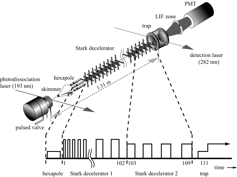
Figure 1: Scheme of the experimental setup. A pulsed beam of OH radicals with a mean velocity of 360 m/s is produced via ArF-laser photodissociation of HNO₃ seeded in Xe. The molecules pass through a skimmer, a hexapole, and a Stark decelerator and are subsequently confined in an electrostatic trap. State-selective LIF detection is performed inside the trap. A schematic representation of the time sequence of high-voltage pulses is shown at the bottom of the figure, including selected indices of the switching times; see text for details.

In brief, a pulsed beam of OH radicals is produced by photodissociation of HNO₃ that is co-expanded with Xe from a pulsed solenoid valve. The mean velocity of the beam is around 360 m/s with a velocity spread (full width at half maximum) of 15 %. After the supersonic expansion, most of the OH radicals in the beam reside in the lowest rotational ($J=3/2$) level in the vibrational and electronic ground state $X\,^{2}\Pi_{3/2},v=0$. The molecular beam passes through a skimmer with a 2 mm-diameter opening and is transversely focused into the Stark decelerator using a short pulsed hexapole. The Stark decelerator consists of an array of 109 equidistant pairs of electrodes, with a center-to-center distance of 11 mm. The decelerator is operated using a voltage difference of 40 kV between opposing electrodes, creating a maximum electric field strength on the molecular beam axis of about 90 kV/cm. A kinetic energy of 0.9 cm^-1 is extracted from the OH molecules per deceleration stage (the region between adjacent pairs of electrodes), and part of the beam is decelerated from 371 to 79 m/s after 101 stages. In the remainder of this paper, these first 101 stages will be referred to as decelerator 1. The last seven stages of the decelerator, referred to as decelerator 2, are electronically and mechanically decoupled from decelerator 1, and are used at a lower voltage difference of $30$ kV. Here, the molecules are decelerated further to a velocity of $21$ m/s, prior to the loading of the packet into the electrostatic trap. The trap consists of two hyperbolic endcaps and a ring electrode. To load the molecules into the trap its electrodes are switched from an initial loading configuration to a trapping configuration. The loading configuration creates a potential hill that is higher than the kinetic energy of the molecules. The OH radicals, therefore, come to a standstill while flying into the trap. At this moment the electrodes are switched to the trapping configuration, creating a field minimum in the center of the trap.

The number of trapped OH radicals as well as the temperature of the trapped gas critically depend on the details of the trap-loading sequence, and in particular on the velocity with which the molecules enter the trap van de Meerakker et al. (2005). If this velocity is chosen such that the molecules come to a standstill exactly at the center of the trap (v$=15$ m/s), a distribution corresponding to a temperature of $50$ mK can be reached. If this velocity is larger, the molecules come to a standstill past the center of the trap, and the final temperature is higher. The reduced spreading out of a faster beam while flying from the last stage of the decelerator to the trap, however, results in a larger number of trapped molecules. The velocity of 21 m/s and the subsequent trap-loading sequence that is used as reference for the optimization in the present experiment are identical to the trap-loading that was used in previous OH trapping experiments van de Meerakker et al. (2005). It results in a temperature of the trapped molecular packet of about 450 mK, an estimated number density of $10^{7}-10^{8}$ molecules per cm³, and a trapping lifetime of $1.6$ s.

The OH radicals are state selectively detected in the trap using a laser-induced fluorescence (LIF) detection scheme. The 282 nm UV radiation of a pulsed dye laser excites the $A\,^{2}\Sigma^{+},v=1\longleftarrow{}X\,^{2}\Pi_{3/2},v=0$ transition. A photomultiplier tube (PMT) is used to measure the resulting off-resonant fluorescence. In the experiments reported here, the repetition rate of the experiment is 10 Hz and for every datapoint 64 successive measurements are averaged. The signal-to-noise ratio of the trapping experiment under these conditions is about 20.

II.2 Feedback control optimization

As described in section II.1 the individual timings in the time sequences applied to the machine are very critical. Generally, initial time sequences are calculated based on a theoretical model of the experiment and will be referred to as calculated time sequences throughout this paper.

For the feedback control optimization the LIF intensity of trapped OH molecules, as described above, is used. To avoid effects from the oscillations of the molecular packet inside the trap that appear during the first milliseconds after switching on the trap (see Fig. 3 of van de Meerakker et al. (2005) and Fig. 4 of this paper), the LIF intensity is measured after $20$ ms trapping-time. This measurement of the OH density in the trap is used as objective function (fitness) in the feedback control algorithm. Since the lifetime of the OH radicals confined in the trap is as long as $1.6$ s, the number of detected OH molecules after 20 ms is still $>98$ % of the maximum value. Because the LIF signal at that detection time is practically constant over periods much longer than the timing changes due to the feedback control algorithm ($\ll{}1$ ms), pulsed laser excitation at a fixed time can be applied for the molecule detection. Note that in the feedback control loop implemented here, we use the result from previous experimental runs as feedback for following ones.

This given problem requires the optimization in a large parameter space, which at the same time can only be sampled by a slow and noisy evaluation. For such problems evolutionary algorithms are generally a good choice and have been applied successfully in many fields. The individual parameters to be adjusted are the timings $t_{i}$ that determine the exact switching of the high voltages energizing the deceleration and trapping electrodes. For the given experiment this results in 111 parameters to be optimized. For a detailed depiction of the timing numbering see Fig. 1. To reduce the high dimensionality of the parameter space, we retracted from optimizing all parameters individually, but encoded them in three reduced sets of parameters: The timings of decelerator 1 and the first four timings of decelerator 2 are not optimized independently, but described by two sets of polynomial expansion coefficients. We found that an accurate encoding of the time sequence itself requires a polynomial of high order, i. e., orders larger than 20 for a 5 $\mu$s accuracy. To allow for smaller polynomial orders $o_{1}$ and $o_{2}$ for the two parts of the decelerator, we have only encoded the differences to the calculated time sequence $t_{i}-t_{i,0}$ in the polynomial, allowing for considerably smaller expansions, since they only need to describe deviations from the theoretical timings. For decelerator 1, one obtains timings $t_{i}$ with $i=1$–$102$

$$t_{i}=t_{i,0}+\sum_{j=0}^{o_{\text{1}}}p_{j+1}\cdot(i-1)^{j}$$ (1)

and for decelerator 2 timings $t_{i}$ with $i=103$–$106$

$$t_{i}=t_{i,0}+\sum_{j=0}^{o_{\text{2}}}p_{j+o_{1}+2}\cdot(i-103)^{j}$$ (2)

The remaining five timings $t_{i}$ for the last deceleration stages and the trap-loading and trapping configurations, which are the most critical timings, are optimized individually and independently. To decouple them from the changes of earlier timings, they are encoded as time difference to their respective preceding timing, i. e., we use

$$\Delta{}t_{i}=t_{i}-t_{i-1}=p_{i+o_{1}+o_{2}-104}$$ (3)

for $i=107$–$111$. The complete parameter vector used in the optimization is then encoded as

$$\vec{P}={\left(p_{1},p_{2},\ldots{}p_{o_{1}+o_{2}+7}\right)^{T}\in\left(\mathbb{R}^{+}\right)^{o_{1}+o_{2}+7}}$$ (4)

Typically we have used polynomials of order $o_{1}=2$ for decelerator 1 and order $o_{2}=1$ for decelerator 2, resulting in a parameter vector of length ten. In this way, the dimension of the parameter space is reduced by one order of magnitude compared to the initial one, while control over the whole beamline by the feedback loop is maintained.

With the intuitive representation of the individuals of the optimization problem as a vector of real numbers over a continuous parameter space, the choice of evolutionary strategies is a natural one. ES is an EA dialect that uses a representation of real-valued vectors and generally uses self-adaptivity Eiben and Smith (2003). In the experiments described here, we used the Evolving Object (EO) framework Keijzer et al. (2002); EO: implementation of the ES. As a trade-off between problem size in the ES and theoretical convergence, the eoEsStdev ES strategy, applying uncorrelated mutations with individual step sizes, was used (Eiben and Smith, 2003, section 4.4.2). In this self-adaptive strategy the genotype is a vector of real numbers containing the actual optimization parameters as well as individual mutation widths $\sigma_{i}$ for every parameter $p_{i}$.

The initial optimization meta-parameters used were based on the suggestions by Eiben and Smith Eiben and Smith (2003) and successively adopted according to their success in the experiments. In the most successful optimization runs the following parameters were used: typically a population size of five or ten individuals was used, with population sizes up to 40 in some runs. Typically 30 offsprings were generated every generation, with values ranging from the actual population size to six times the population size over different runs. Generally, an offspring-to-population ratio of seven is assumed to work best, but the theoretical advantage is apparently outweighed by the slowness of the evaluation and the corresponding experimental difficulties in this experiment. The most successful mutation and crossover rates were 75 % and 50 %, respectively, but this seems not to be critical and was not tested extensively. Parent selection was done using the ordered sequential selector. We have used discrete global recombination for the experimental parameters and intermediate global recombination for the mutation widths $\sigma$. For survivor selection the $(\lambda,\mu)$ approach worked best, as it seems to handle noise and drifts in the experimental conditions well, as is generally assumed (Eiben and Smith, 2003, section 4.7). Elitism was not applied.

This machine learning is implemented in our data-acquisition system (KouDA) using ES within an automatic feedback control loop.

III Experimental results

In Fig. 2 the normalized average fitness — the LIF signal from OH radicals in the trap — per generation is plotted against the generation number for three different optimization runs, referred to as runs A, B, and C. The measured fitness-values are normalized with respect to the fitness obtained for the calculated time sequence under the same experimental conditions. In each run, different strategy parameters for the algorithm or different initial populations are used, as detailed below. Typically, a complete optimization run corresponds to the evaluation of many hundred generated time sequences and takes about 1–2 h of measuring time.

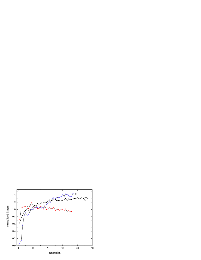
Figure 2: (Color Online): For three different optimization runs, each with different initial parameters, the normalized average fitness per generation is plotted. Curves A (squares) and B (asterisks) show an increase of 30 and 40 %, respectively. During the measurement represented by curve C (triangles) drifts in the experimental conditions, namely the backing pressure of the supersonic expansion, occurred and led to reduced signal intensities, as was confirmed after the optimization run.

In run A (squares), the calculated time sequence is used as starting point for the optimization. From this sequence, an initial population is created with parameters that are randomly picked out of a Gaussian distribution around the calculated values. The last parameter, $\Delta{}t_{111}$, has been decreased by 27 $\mu$s based on the outcome of earlier runs (not presented). As a result of these small changes, the first generation has a slightly lower fitness. After nine generations the average fitness of the generation has increased to the value of the calculated time sequence. For later generation numbers the fitness increases further and reaches a maximum of 1.3 after 46 generations. In the measurement represented by curve B (asterisks) an initial population was created from the same calculated time sequence, but nine out of ten parameters were set off by 3 to 20 %. Hence, the first generation time sequences lead to a normalized fitness of less than 0.1. After 11 generations this number already reaches 1 and is further optimized to 1.4 in generation 37. The optimization runs A and B result in a number of trapped OH radicals that is 30 to 40 % higher than the number that is obtained with the calculated time sequence. Other experiments in which different initial populations were chosen led to a similar increase in the number of trapped molecules.

The initial population and strategy parameters, which are used in the optimization run shown in curve C (triangles), are very similar to the parameters that were used in curve A. Curve C initially shows (as expected) an optimization similar to that of run A and reaches a maximum of 1.2 after around nine generations. From then on, however, the fitness starts decreasing. This is due to a drift in the production of OH radicals during this experimental run, that was confirmed by an independent measurement after the optimization run. In spite of this drift the algorithm still converged and the time sequences obtained for the last generation are comparable with time sequences obtained in runs A and B (vide infra).

Other experiments using different strategy parameters for the ES, for example, different population sizes or different settings for mutation and crossover rates, did lead to a similar increase in the number of trapped molecules of 35–40 %. Furthermore, the values of corresponding parameters from the optimized time sequences are generally comparable. These results show not only that the algorithm is able to optimize the number of trapped molecules, but also that it finds a reproducible maximum in the parameter-space, even if the initial parameters deviate significantly or external factors disturb the experiment.

The evolutions of three of the most important parameters, recorded during optimization run A, are shown in Fig. 3. Fig. 3 a and 3 b show $\Delta{}t_{108}$ and $\Delta{}t_{109}$, respectively. These parameters define the switching times of the last two stages of decelerator 2 and thus determine the exact velocity with which the molecules leave the decelerator. Fig. 3 c depicts the evolution of $\Delta{}t_{111}$, the time interval during which the loading configuration of the trap is used. At the end of this time interval the trapping configuration is switched on. For reference, the horizontal lines in the plots denote the mean value of the respective parameter in the first generation, which are equivalent to the parameters in the calculated time sequence. Although the fitness depends very critically on these specific timings, the evolution of the parameters shown in Fig. 3 is typical for the evolution of less critical parameters as well.

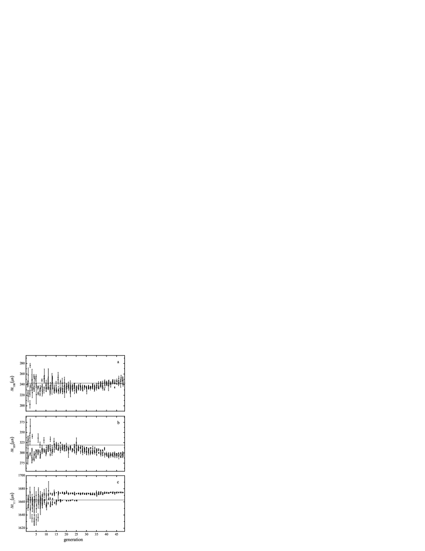
Figure 3: The evolution of three of the parameters during optimization run A (see Fig. 2): a) $\Delta{}t_{108}$, b) $\Delta{}t_{109}$, c) $\Delta{}t_{111}$. The squares mark the value of individual parameters and the error bars represent the corresponding mutation widths $\sigma$. Only the five parameters selected for a new population (as described in section II.2) are shown and they are grouped by generation. Individual parameters within a population are slightly offset horizontally to allow the observation of individual values and their error bars. At the beginning, a large range of the parameter space is searched, whereas later in the optimization the $\sigma$’s are reduced by the algorithm and convergence is reached. The horizontal lines denote the mean value of each parameter in the first generation.

For all three parameters, the mutation widths $\sigma$, represented by the vertical bars, are initially large and the parameters scatter over a relatively large range. As the generation number increases, this mutation width decreases and the parameters converge. Parameter $\Delta{}t_{111}$, however, converges initially to two values, one centered around 1662 $\mu$s, the other around 1674 $\mu$s. This shows that the parameter-space contains multiple local maxima, and that multiple pathways in the parameter-space can be followed. Only after 27 generations, exclusively individuals with a value for $\Delta{}t_{111}$ of about 1674 $\mu$s survive the selection. As most runs converge to similar values this seems to be the global optimum, at least for the parameter space searched.

From each feedback control experiment a set of optimized time sequences is obtained. It is clear from the optimized time sequences, that no different mode of operation for the Stark decelerator is obtained and that the previous theoretical understanding Bethlem et al. (2002) is confirmed by these experiments. Moreover, comparing the time-of-flight (TOF) profiles of OH radicals at the center of the trap, which are measured using the calculated and optimized time sequences, a physical interpretation of the differences can be deduced.

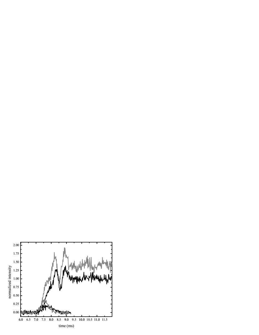
Figure 4: Density of OH radicals at the center of the trap as a function of time after their production. The lower two traces are the intensities of molecules passing through the center of the trap without any voltages applied to the trap electrodes. The upper traces are measurements for trapping experiments. The black traces are measured with the calculated time sequence applied to the machine, whereas the gray traces are measured with one of the generated, optimized time sequences obtained from automated optimization using evolutionary strategies.

The typical result of such a measurement is shown in Fig. 4. The black and gray curves are measured using the calculated and optimized time sequences, respectively. The lower two curves show the TOF profiles of the OH molecules as they arrive in the trap when no voltages are applied to the trap electrodes. The positions and widths of the arrival-time distributions are a measure for the longitudinal velocity distributions of the decelerated OH beams that exit the decelerator. Compared to the calculated time sequence, the optimized sequence results in an arrival-time distribution that is shifted 180 $\mu$s to the left, indicating that the molecular packet arrives with a higher mean velocity of 25 m/s, instead of 21 m/s, in the trap. Assuming the transverse and longitudinal velocity spreads are unaltered for the optimized time sequence, the beam spreads out less in all directions while traveling the distance from the end of the decelerator to the trap, and the corresponding arrival-time distribution is narrower. The integral of the peak of the arriving packet (lower curves) is already enhanced by about 40 %, reflecting the reduced transverse spreading out of the beam and hence the reduced transverse losses while entering the trap.

The upper two curves show the density of OH radicals at the center of the trap when the trap-loading and trapping electric fields are applied. The optimized time sequence (gray curve) leads to a more pronounced oscillation in the TOF profile than the calculated one (black curve). This is readily understood from the higher initial velocity of the molecules. The molecules enter the trap too fast, and come to a standstill past the center of the trap. The molecular packet is poorly matched to the trap acceptance, and the width of the velocity distribution of the trapped molecules will therefore be larger as well. These results confirm, as was already concluded earlier van de Meerakker et al. (2005), that a large number of molecules in the trap and a low temperature of the trapped packet of molecules are conflicting goals with the present design of the trap: the required low velocity to match the decelerated molecular packet with the acceptance of the trap results in a large transverse spreading out of the packet prior to entering the trap.

In principle, one could also aim a feedback control optimization at determining a time sequence for a trapped molecular packet with a temperature as low as possible, or a weighted combination of the number of trapped molecules and a minimal temperature, by using an appropriate experimental objective function. One could, for example, measure the number of molecules at the center of the trapping region after a predefined time of free expansion of a previously trapped packet. That would result in a combined determination of the peak density of the trapped molecular packet and its temperature, where the time delay between switching off the trap and the detection of the molecular density would weigh the two contributions to the fitness. Alternatively, if the spatial density distribution of the trapped molecular packet would be measured for every generated time sequence, direct information on the number of trapped molecules and their temperature is obtained, allowing to define any objective function based on these two important measures. Furthermore, when using continuous detection to allow for measuring the complete time-of-flight profile from the nozzle to the detection region for every molecular packet, the integrated intensity and the longitudinal temperature can be deduced offline by the optimization algorithm . This allows to optimize any Stark-decelerator beamline, even without trapping.

Besides the timings of the high-voltage pulses one can also optimize other computer controllable experimental parameters, such as the voltages that are applied to the experiment, laser frequencies, etc. In general, evolutionary algorithms can be used for the optimization of any fitness function that can be determined experimentally. This includes, for example, the ratio of molecules simultaneously trapped in two different quantum states or the ratio of decelerated and actually trapped molecules. More generally, the method can also be applied to other atomic and molecular beam experiments, such as optimizing the timings or voltages in multipole focusers Reuss (1988) or the currents in a Zeeman slower Metcalf and van der Straten (1999).

IV Conclusions

In this paper we describe the successful implementation of feedback control optimization of the Stark deceleration and trapping of OH radicals using evolutionary strategies. The time sequence of high-voltage pulses that is applied to the decelerator and trap electrodes is encoded as parameter vector for the algorithm. Starting from an initial time sequence based on an idealized representation of the beamline, the number of trapped OH radicals is increased by 40 %. This enhancement is qualitatively understood in terms of the improved coupling in of the amount of molecules into the trap.

The machine learning approach presented here can be applied to other Stark-deceleration experiments as well. The optimization will be especially useful for all experiments in which very slow molecular beams ($v<100$ m/s) are manipulated, for which the exact switching times of the high-voltage pulses are extremely critical. In general, any computer-controllable experimental parameter can be optimized using evolutionary algorithms and any fitness function that can be determined experimentally can be used as fitness for the optimization.

Essential to the present experiment is the use of trapped molecules, which enables the decoupling of the timing for pulsed laser detection from the optimization. For beamlines with continuous detection such a timing can be evaluated offline and becomes uncritical, thus making feedback control optimization generally applicable.