Regime of Validity of the Pairing Hamiltonian in the Study of Fermi Gases

Abstract

The ground state energy and pairing gap of the interacting Fermi gases calculated by the ab initio stochastic method are compared with those estimated from the Bardeen-Cooper-Schrieffer pairing Hamiltonian. We discuss the ingredients of this Hamiltonian in various regimes of interaction strength. In the weakly interacting ($1/ak_{F}<<0$) regime the BCS Hamiltonian should describe Landau quasi-particle energies and interactions, on the other hand in the strongly pairing regime, that is $1/ak_{F}\gtrsim 0$, it becomes part of the bare Hamiltonian. However, the bare BCS Hamiltonian is not adequate for describing atomic gases in the regime of weak to moderate interaction strength $-\infty<1/ak_{F}<0$ such as $ak_{F}\sim-1$.
PACS: 05.30.Fk, 03.75.Ss, 21.65.+f

The superfluid state of alkali fermion gases such as ⁶Li, ⁴⁰K is analogous to the superconducting state found in the electronic systems bardeen1957 and it has been studied theoretically houbiers97 and experimentally gupta03 . Recent experimental progress includes the detection of the Bose Einstein Condensate (BEC) state of the bound Fermi pairs regal2003 ; regal2004 ; bartenstein2004 ; zwierlein2004 as an evidence of the predicted BCS-BEC crossover.

The interaction among ⁶Li atoms can be attractive and requires preparation of the atoms in different internal quantum states $|1\rangle$ and $|2\rangle$. The Feshbach resonance feshbach58 ; feshbach62 ; tiesinga93 between the atoms in these states can modify the characteristics of the collision. We assume that the partial densities of the atomic species are the same and the temperature is low ($T\approx 0$). The interactions can be characterized by the s-wave scattering length $a$ which can be tuned by the externally applied magnetic field. The Hamiltonian of the interacting atomic fermions can be written in the configuration space as

$${\cal H}^{bare}=-\frac{\hbar^{2}}{2m}\sum\limits_{p=1}^{N}\nabla^{2}_{p}+\sum_{i,i^{\prime}}V(r_{ii^{\prime}})$$ (1)

where the index $i$ is for species $|1\rangle$ particles while $i^{\prime}$ is for species $|2\rangle$ particles. In the momentum space, the Hamiltonian can be written as

$${\cal H}^{bare}=\sum_{\sigma,\bf k}\frac{\hbar^{2}k^{2}}{2m}a^{\dagger}_{\sigma,\bf k}a_{\sigma,\bf k}+\frac{1}{2}\sum_{{\bf k},{\bf k}^{\prime},{\bf q}}v^{B}_{{\bf k},{\bf k}^{\prime},{\bf q}}a^{\dagger}_{1,{\bf k}+{\bf q}}a^{\dagger}_{2,{\bf k}^{\prime}-{\bf q}}a_{2,{\bf k}^{\prime}}a_{1,{\bf k}}$$ (2)

with $a^{\dagger}_{\sigma,\bf k}$ and $a_{\sigma,\bf k}$ being particle operators. This is the so-called bare Hamiltonian.

On the other hand, in terms of the quasi-particles, we have the so-called Landau Hamiltonian of the form

$${\cal H}^{Landau}=E_{N}+\sum_{\sigma,\bf k}\left[\epsilon^{Q}_{\bf k}-\mu_{c}\right]c^{\dagger}_{\sigma,\bf k}c_{\sigma,\bf k}+\frac{1}{2}\sum_{{\bf k},{\bf k}^{\prime},{\bf q}}v^{Q}_{{\bf k},{\bf k}^{\prime},{\bf q}}c^{\dagger}_{1,{\bf k}+{\bf q}}c^{\dagger}_{2,{\bf k}^{\prime}-{\bf q}}c_{2,{\bf k}^{\prime}}c_{1,{\bf k}}~{},$$ (3)

where $c^{\dagger}_{\sigma,\bf k}$ and $c_{\sigma,\bf k}$ are quasi-particle operators, $E_{N}\equiv$ energy of the ‘normal’ ground state, $\epsilon^{Q}_{\bf k}\equiv$ quasi-particle energy spectrum, and $\mu_{c}\equiv E_{F}$. In general, we have $v^{Q}_{{\bf k},{\bf k}^{\prime},{\bf q}}\neq v^{B}_{{\bf k},{\bf k}^{\prime},{\bf q}}$.

Further simplification yields BCS pairing Hamiltonian that can also be written in two ways

$${\cal H}_{BCS}^{bare}=\sum_{\sigma,\bf k}\frac{\hbar^{2}k^{2}}{2m}a^{\dagger}_{\sigma,\bf k}a_{\sigma,\bf k}+\sum_{{\bf k},{\bf k}^{\prime}}v^{B}_{{\bf k},{\bf k}^{\prime}}a^{\dagger}_{1,{\bf k}}a^{\dagger}_{2,-{\bf k}}a_{2,-{\bf k}^{\prime}}a_{1,{\bf k}^{\prime}}$$ (4)

and

$${\cal H}_{BCS}^{Landau}=E_{N}+\sum_{\sigma,\bf k}\left[\epsilon^{Q}_{\bf k}-\mu_{c}\right]c^{\dagger}_{\sigma,\bf k}c_{\sigma,\bf k}+\sum_{{\bf k},{\bf k}^{\prime}}v^{Q}_{{\bf k},{\bf k}^{\prime}}c^{\dagger}_{1,{\bf k}}c^{\dagger}_{2,-{\bf k}}c_{2,-{\bf k}^{\prime}}c_{1,{\bf k}^{\prime}}$$ (5)

The BCS approach is to restrict the interaction to the time-reversed pair (${\bf k}$,$-{\bf k}$) of different species.

Ground states of Hamiltonian (Eq 1) have been obtained using the stochastic method known as Green’s Function Monte Carlo (GFMC) carlson2003 ; chang2004 where variational degrees of freedom were introduced to deal with the fermion sign problem. Their energies are considered as close upper bounds to those of the exact ground state. In the Ref carlson2003 ; chang2004 , a finite short range cosh-function potential rather than $\delta$-function potential was used. The range of the potential is $\sim\frac{1}{6}r_{0}$ where $r_{0}$ is the unit radius ($\frac{4}{3}\pi r_{0}^{3}\rho=1$). From the results of the lowest order cluster calculations known as LOCV vijay71 ; vijay73 (Lowest Order Constrained Variational) it appears that this finite range potential is a good approximation for the zero range potential in the $1/ak_{F}<0$ regime (see Fig 1).

$\frac{1}{ak_{F}}$	$\mu_{c}$	$\Delta_{BCS-Leggett}$	$\Delta_{GFMC}$	$E_{BCS-Leggett}$	$\Delta E$
-1.5	1.65	0.16		0.99	0.15
-$1.\dot{3}$	1.65	0.20		0.99	0.15
-1.0	1.53	0.33	0.29	0.98	0.19
-0.5	1.45	0.65		0.90	0.18
-$0.\dot{3}$	1.35	0.78	0.77	0.83	0.18
-0.1	1.15	1.02	0.87	0.69	0.17
0.0	1.03	1.13	0.99	0.60	0.16
0.1	0.90	1.25	1.03	0.50	0.16
$0.\dot{3}$	0.58	1.58	1.4	0.24	0.22
0.5	0.17	1.75	1.8	-0.12	0.22
1.0	-1.50	2.35	3.2	-1.56	0.67

Table 1: Comparison of Leggett results with ${\cal H}_{BCS}^{bare}$ vs GFMC. The unit of energy is $E_{FG}=\frac{3}{5}\frac{\hbar^{2}k_{F}^{2}}{2m}$. We notice $E_{F}=1.67E_{FG}$. We define $\Delta E\equiv E_{BCS-Leggett}-E_{GFMC}$. We notice that while there is considerable discrepancy in the energies, the gaps are in reasonable match for $1/ak_{F}<-1/3$. Errors are in the last digit except for $\Delta_{GFMC}$ where the relative error $\sim 10\%$.

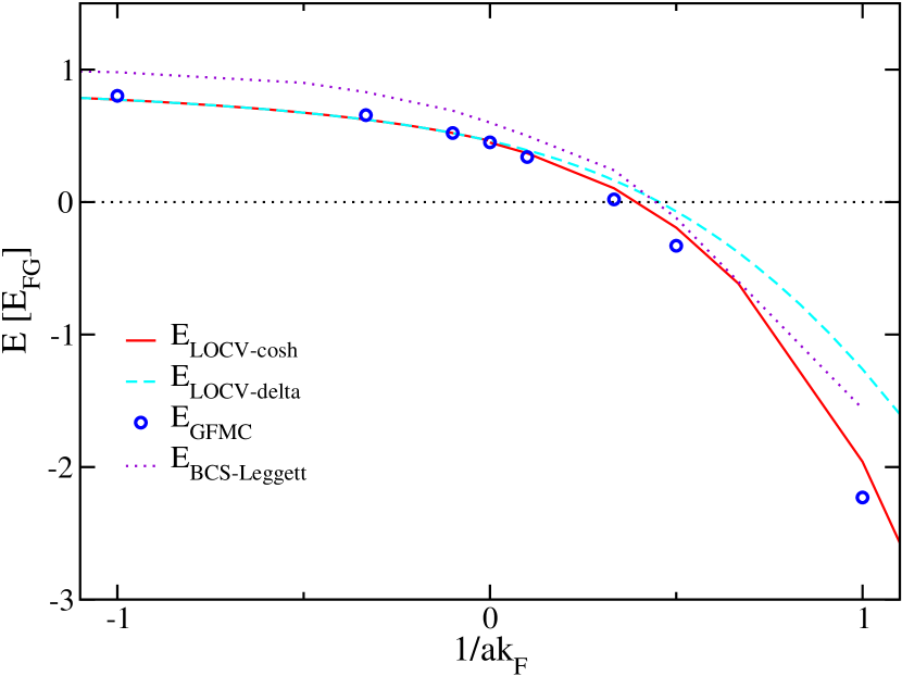
Figure 1: Comparison of $E/N$ calculated using different methods. Both finite range ‘cosh’ potential and $\delta$-function like potentials are considered for the LOCV calculations.

The original BCS technique was to use ${\cal H}_{BCS}^{Landau}$ (Eq 5) and solve it variationally using $\Psi_{BCS}$. The solution will give the superfluid energy $E_{S}=E_{N}+E_{P}$, where the pairing energy $E_{P}=-N_{0}\frac{\Delta^{2}}{2}$. In general, it is difficult to obtain analytically ${\cal H}^{Landau}_{BCS}$ from ${\cal H}^{bare}_{BCS}$. However, for weak potential strength, that is $1/ak_{F}<-1$, we can map the ${\cal H}^{bare}_{BCS}$ into ${\cal H}^{Landau}_{BCS}$ by making the substitution

$$E_{N} = E_{Lenz}$$ (6)

$$\epsilon^{Q}_{\bf k} = \frac{\hbar^{2}k^{2}}{2m}+const.$$ (7)

$$v^{Q}_{{\bf k},{\bf k}^{\prime}} \approx v^{B}_{{\bf k},{\bf k}^{\prime}}$$ (8)

In this case we can get $E_{S}=E_{N}+E_{P}=E_{Lenz}+E_{P}$ (see Fig 2). This projection of the bare Hamiltonian into the Landau Hamiltonian is useful only in the weak interaction limit in which $E_{Lenz}-E_{FG}$ has most of the interaction effect and $|E_{p}|<<|E_{Lenz}-E_{FG}|$ as seen in the Fig 2.

On the other hand, Leggett leggett1980 ; parish2005 solved the ${\cal H}_{BCS}^{bare}$ (Eq 4) with the condition that the density remains constant with the chemical potential $\mu_{c}$ adjusted accordingly. This method can be applied in all regimes of interaction. The interaction of the Hamiltonian assumes zero range $v^{B}_{{\bf k},{\bf k}^{\prime}}\rightarrow g=\frac{4\pi\hbar^{2}a}{m\Omega}$ ($\Omega=$ volume) adequate for the dilute regime where the potential range $R$ and $a$ are much less than $r_{0}\sim\frac{1}{k_{F}}$ as well as the ‘intermediate’ regime where $R<<r_{0}<<a$. From $n_{\bf k}=|v_{\bf k}|^{2}=\frac{1}{2}\left[1-\frac{\epsilon_{\bf k}-\mu_{c}}{E_{\bf k}}\right]$, we can draw the normalization condition. Going to the continuum limit and expressing in the units of $E_{F}=\frac{\hbar^{2}k_{F}^{2}}{2m}$, we have a set of two equations

$$\int_{0}^{\infty}d\epsilon\epsilon^{1/2}\left[1-\frac{\epsilon-\mu_{c}}{\sqrt{(\epsilon-\mu_{c})^{2}+\Delta^{2}}}\right]=\frac{4}{3}$$ (9)

$$\int_{0}^{\infty}d\epsilon\epsilon^{1/2}\left[\frac{1}{\epsilon}-\frac{1}{\sqrt{(\epsilon-\mu_{c})^{2}+\Delta^{2}}}\right]=\frac{\pi}{ak_{F}}$$ (10)

where Eq 10 comes from subtracting the equation for the scattering length $a$ (see Ref papenbrock99 )

$$-\frac{mg\Omega}{4\pi a\hbar^{2}}+1=-\frac{g\Omega}{2(2\pi)^{3}}\int\limits_{0}^{\infty}4\pi k^{2}dk\frac{1}{\epsilon(k)}$$ (11)

from the gap equation

$$1=-\frac{g\Omega}{2(2\pi)^{3}}\int\limits_{0}^{\infty}4\pi k^{2}dk\frac{1}{\sqrt{(\epsilon(k)-\mu_{c})^{2}+\Delta^{2}}}~{}.$$ (12)

The $\mu_{c}$ and $\Delta$ are solved simultaneously. The solutions are given in the Table 1. In this table, the energy per particle $E_{BCS-Leggett}=E/N$ was estimated using $\mu_{c}$ and $\Delta$, and the expression

$$E/N=\frac{1}{N}\sum_{\bf k}2\epsilon_{\bf k}|v_{\bf k}|^{2}-\Delta u_{\bf k}v_{\bf k}$$ (13)

with the usual definitions of $\Delta=-g\sum\limits_{\bf k}u_{\bf k}v_{\bf k}$ and $|u_{\bf k}|^{2}=1-|v_{\bf k}|^{2}$.

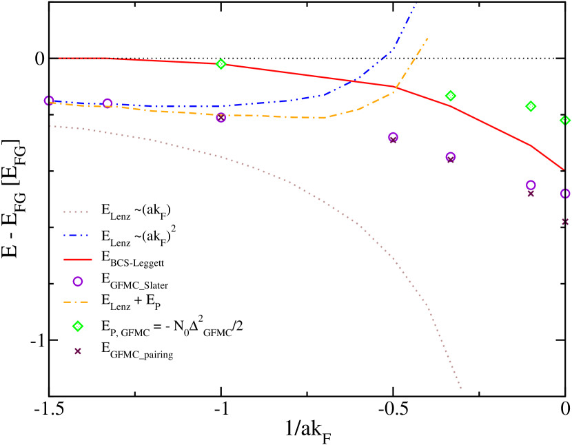
Figure 2: Comparison of $E/N$ and $\Delta$ calculated using BCS-Leggett equations and the stochastic GFMC method. The $E_{FG}$ is subtracted from all energies. Second order $E_{Lenz}$ and $E_{P}=-N_{0}\frac{\Delta_{BCS-Landau}}{2}$ were used to plot $E_{S}\equiv E_{Lenz}+E_{P}$. $E_{S}$ has good match with $E_{GFMC}$ up to $1/ak_{F}\approx-1$.

In the Fig 2, we compare the normal phase low density Lenz expansion lenz1929 ; huang1957 ; galitskii1958

$$\frac{E}{NE_{FG}}=1+\frac{10}{9\pi}ak_{F}+\frac{4}{21\pi^{2}}(11-2ln2)(ak_{F})^{2}+\cdots$$ (14)

of first and second order of $ak_{F}$ with BCS-Leggett and GFMC results both from the bare potential. The Lenz expansion is considered exact in the low density regime for the interacting Fermi gas in normal phase. From Fig 2, it is obvious that the expansion diverges for $1/ak_{F}>-1$ . $E_{S}=E_{Lenz}+E_{P}$ has good match with the GFMC results in the regime $1/ak_{F}\lesssim-1$. Here the effect of pairing is small in $E_{GFMC}$ (the difference between the Slater node and BCS node solutions lies within the statistical uncertainties) thus $|E_{p}|<<|E_{Lenz}-E_{FG}|$ is a reasonable assumption although $\Delta$ is clearly non zero. In this regime we notice that $E_{BCS-Leggett}$ is distinguishably higher than $E_{GFMC}$ and energies of the normal phase low density expansion. At $ak_{F}=-1$, $\Delta E=E_{BCS-Leggett}-E_{GFMC}=0.19E_{FG}$ (see Table 1). This is a consequence of having the anomalous density $u_{\bf k}v_{\bf k}$ small and $\mu_{c}\approx E_{F}$. In fact, when $u_{\bf k}v_{\bf k}\approx 0$ the $\Psi_{BCS}\rightarrow\Psi_{FG}$. However, we can see that the usual Hartree-Fock term for the normal phase is missing (Eq 13) in the energy expression from the pairing Hamiltonian. Thus we have $E_{BCS-Leggett}$ much higher even than $E_{Lenz}$.

We interpret this as a consequence of using pairing Hamiltonian instead of the full bare interaction Hamiltonian. The pairing Hamiltonian becomes a poor model for the atomic gas in the interacting regime with $-\infty<1/ak_{F}<0$, in particular around the moderate interaction strength $ak_{F}\sim-1$. This is in sharp contrast to the context in which the original Landau-BCS formalism was introduced that was the weak coupling approximation in a broad range $-\infty\leq 1/ak_{F}\lesssim-1$. $E_{GFMC}$, $E_{BCS-Leggett}$, and $E_{Lenz}+E_{P}$ converge in the $ak_{F}\approx 0$ regime, that is the trivial free Fermi gas limit, where the Hartree-Fock term becomes effectively zero.

On the other hand, the time reversed pairing (k,-k) assumption becomes less relevant once the interaction is strong enough for the particles to form loosely bound pairs in the sea of many fermions. This can be seen as $\Delta E$ becomes smaller ($=0.15E_{FG}$) in the strongly interacting regime $1/ak_{F}=0$ and $1/ak_{F}=+0.1$. In the $1/ak_{F}\geq 0.\dot{3}$ region, $E_{BCS-Leggett}$ and $E_{GFMC}$ apparently reverse back to the diverging behavior (Fig 1). But as shown in the comparison of the LOCV energies, the range of the model potential becomes inadequate to approximate the $\delta$-potential as the size of the bound pairs become $\lesssim r_{0}$ and $\sim R$. We argue that the actual $E_{GFMC}$ with short range potential would lie closer to $E_{BCS-Leggett}$ than the current finite range calculation shows. The bound fermions condense in the ${\bf k}={\bf 0}$ state. Thus ${\cal H}_{atom}^{bare}$ (Eq 2) $~{}\rightarrow~{}{\cal H}_{BCS}^{bare}$ (Eq 4) and results of two models should match.

As for the pairing gap, both BCS-Leggett and GFMC results seem to be in reasonable agreement in the whole $1/ak_{F}<0$ region considering that statistical errors of $\Delta_{GFMC}\sim 10\%$. The reasonable match of $\Delta$ while a poorer match for $E/N$ is not surprising given the fact that the chemical potential $\mu_{c}$ is greatly modified in this region. $\mu_{c}$ goes from $\sim E_{F}=\frac{\hbar^{2}k_{F}^{2}}{2m}=1.67E_{FG}$ at $1/ak_{F}\approx-1$ to the $\mu_{c}<0$ for $1/ak_{F}\gtrsim 0.5$ where zero momentum excitation is possible and BEC is achieved.

In conclusion, we have tested the regimes of validity of the BCS pairing Hamiltonian in the study of fermion particles interacting with bare short-range two-body potential. We notice that the pairing assumption is generally not valid when bare potential is used in a broad range of the weakly interacting regime $-\infty<1/ak_{F}<0$, while the original quasi-particle BCS formalism was introduced to describe the superfluid precisely in this region.We notice considerable discrepancy in the energy, however the gap is predicted with reasonable accuracy at $ak_{F}\approx-1$. Pairing correlation is less relevant in the trivial (free Fermi gas) and the tightly bound pair ($1/ak_{F}>0$) limits. In fact, it can be shown that GFMC calculations with both Slater and pairing nodes converge to the same value (molecular energy per particle $E_{mol}/2$) in the extreme of this limit. This work has been supported in part by the US National Science Foundation via grant PHY 00-98353 and PHY 03-55014. The authors thank useful comments from Prof. G. Baym of UIUC and J. Carlson of LANL.

References

(1)
J. Bardeen,
L. N. Cooper,and
J. R. Schrieffer,
Phys. Review 108,
1175 (1957).
(2)
M. Houbiers,
R. Ferwerda,
H. T. C. Stoof,
W. I. McAlexander,
C. A. Sackett,
and
R. G Hulet,
Phys. Rev. A 56,
4864 (1997).
(3)
S. Gupta,
Z. Hadzibabic,
M. W. Zwierlein,
C. A. Stan,
K. Dieckmann,
C. H. Schunck,
E. G. M. van Kempen,
B. J. Verhaar,
and
W. Ketterle,
Science 300,
1723 (2003).
(4)
C. A. Regal,
C. Ticknor,
J. L. Bohn, and
D. S. Jin,
Nature 424,
47 (2003).
(5)
C. A. Regal,
M. Greiner, and
D. S. Jin,
Phys. Rev. Lett. 92,
040403 (2004).
(6)
M. Bartenstein,
A. Altmeyer,
S. Riedl,
S. Jochim,
C. Chin,
J. H. Denschlag,
and
R. Grimm,
Phys. Rev. Lett. 92,
120401 (2004).
(7)
M. W. Zwierlein,
C. A. Stan,
C. H. Schunck,
S. M. F. Raupach,
A. J. Kerman,
and
W. Ketterle,
Phys. Rev. Lett. 92,
120403 (2004).
(8)
H. Feshbach,
Ann. Phys. 5,
357 (1958).
(9)
H. Feshbach,
Ann. Phys. 19,
287 (1962).
(10)
E. Tiesinga,
B. J. Verhaar,
and
H. T. C. Stoof,
Phys. Rev. A 47,
4114 (1993).
(11)
J. Carlson,
S. Y. Chang,
V. R. Pandharipande,
and
K. E. Schmidt,
Phys. Rev. Lett. 91,
50401 (2003).
(12)
S. Y. Chang,
V. R. Pandharipande,
J. Carlson,
and
K. E. Schmidt,
Phys. Rev. A 70,
043602 (2004).
(13)
V. R. Pandharipande,
Nucl. Phys. A 174,
641 (1971).
(14)
V. R. Pandharipande,
and H. A.
Bethe,
Phys. Rev. C 7,
1312 (1973).
(15)
A. J. Leggett, in
Modern Trends in the Theory of Condensed Matter,
edited by A. Pekalski
and R. Przystawa
(Springer-Verlag, Berlin,
1980).
(16)
M. M. Parish,
B. Mihaila,
E. M. Timmermans,
K. B. Blagoev,
and
P. B. Littlewood,
Phys. Rev. B 71,
064513 (2005).
(17)
T. Papenbrock and
G. F. Bertsch,
Phys. Rev. C
59, 2052 (1999).
(18)
W. Lenz,
Z. Physik 56,
778 (1929).
(19)
K. Huang, and
C. N. Yang,
Phys. Rev. 105,
767 (1957).
(20)
V. M. Galitskii,
Sov. Phys. JETP 7,
104 (1958).