Living in an Irrational Society: Wealth Distribution with Correlations between Risk and Expected Profits

Abstract

Different models to study the wealth distribution in an artificial society have considered a transactional dynamics as the driving force. Those models include a risk aversion factor, but also a finite probability of favoring the poorer agent in a transaction. Here we study the case where the partners in the transaction have a previous knowledge of the winning probability and adjust their risk aversion taking this information into consideration. The results indicate that a relatively equalitarian society is obtained when the agents risk in direct proportion to their winning probabilities. However, it is the opposite case that delivers wealth distribution curves and Gini indices closer to empirical data. This indicates that, at least for this very simple model, either agents have no knowledge of their winning probabilities, either they exhibit an “irrational” behavior risking more than reasonable.

A study of the distribution of the income of workers, companies and countries was presented, more than a century ago, by Italian economist Vilfredo Pareto. He investigated data of income for different European countries and found a power law distribution that seems to be independent on particular economic condition of each country. He found Pareto that the distribution of income and wealth follows a power law behavior where the cumulative probability $P(w)$ of people whose income is at least $w$ is given by $P(w)\propto w^{-\alpha}$, where the exponent $\alpha$ is named today Pareto index. The exponent $\alpha$ for several countries was $1.2\leq\alpha\leq 1.9$. However, recent data indicate that, even though Pareto’s law provides a good fit to the distribution of the high range of income, it does not agree with observed data over the middle and low range of income. For instance, data from Japan souma , the United States of America and the United Kingdom dragu2000 ; dragu2001a ; dragu2001b are fitted by a lognormal or Gibbs distribution with a maximum in the middle range plus a power law for the highest income. The existence of these two regimes may be qualitatively justified by stating that in the low and middle income classes the process of accumulation of wealth is additive, causing a Gaussian-like distribution, while in the high income class the wealth grows in a multiplicative way, generating the power law tail.

Different models of capital exchange among economic agents have been recently proposed. Most of these models consider an ensemble of interacting economic agents that exchange a fixed or random amount of a quantity called “wealth”. In the model of Dragulescu and Yakovenko dragu2000 ; review this parameter is associated with the amount of money a person has available to exchange, i. e. a kind of economic “energy” that may be exchanged by the agents in a random way. The resulting wealth distribution is a Gibbs exponential distribution, as it would be expected. An exponential distribution as a function of the square of the wealth is also obtained in an extremal dynamics model where some action is taken, at each time step, on the poorest agent, trying to improve its economic state PIAV2003 ; IGPVA2003 . In the case of this last model a poverty line with finite wealth is also obtained, describing a way to diminish inequalities in the distribution of wealth SI2004 . In order to try to obtain the power law tail several methods have been proposed. Keeping the constraint of wealth conservation a detailed studied proposition is that each agent saves a fraction - constant or random - of their resources review . One possible result of those models is condensation, i.e. the concentration of all the available wealth in just one or a few agents. To overcome this situation different rules of interaction have been applied, for example increasing the probability of favoring the poorer agent in a transaction IGPVA2003 ; IGVA2004 ; west1 ; west2 , or introducing a cut-off that separates interactions between agents below and above a threshold Das . Most of these models are able to obtain a power law regime for the high-income class, but for a limited range of the parameters, while for the low income, the regime can be approximately fitted by an exponential or lognormal function. However, in all those models the risk-aversion (or saving propensity) of the agents is determined at random with no correlation with the probability of winning in a given interaction. Also, possible correlations between wealth and probability of interaction are not considered.

Here we assume that the agents have some previous knowledge of their winning probability and they adjust their risk-aversion factor in correlation with this winning probability. As in previous models we consider a population of $N=10^{5}$ interacting agents characterized by a wealth $w_{i}$ and a risk aversion factor $\beta_{i}$. We chose as initial condition for $w_{i}$ a uniform distribution between $0$ and $1000$ arbitrary units. For each agent $i$, the number $[1-\beta_{i}]$ measures the percentage of wealth he is willing to risk. At each time step $t$ we select at random the two agents $i$ and $j$ that will exchange resources. Then, we set the quantity to be exchanged between these two agents as the minimum of the available resources of both agents, i.e., $dw=\min[(1-\beta_{i})w_{i}(t);(1-\beta_{j})w_{j}(t)]$. Finally, following previous works we consider a probability $p\geq 0.5$ of favoring the poorer of the two partners IGVA2004 ; west1 ,

$$p=\frac{1}{2}+f\times\frac{|w_{i}(t)-w_{j}(t)|}{w_{i}(t)+w_{j}(t)},$$ (1)

where $f$ is a factor going from $0$ (equal probability for both agents) to $1/2$ (highest probability of favoring the poorer agent). Thus, in each interaction the poorer agent has probability $p$ of earn a quantity $dw$, whereas the richer one has probability $1-p$. Now we consider that in each transaction both participants know this probability and adjust their risk-aversion $\beta$ according to the value of $p$. If the agents are “rational” they will risk more when they have a higher probability of winning so, taking into account that $p$ varies between $0.5$ and $1$, we first consider that in each interaction:

$$\beta_{rich} = 2\alpha_{r}(p-0.5),$$

$$\beta_{poor} = 2\alpha_{p}(1-p),$$ (2)

with $\alpha_{r}$ and $\alpha_{p}$ ranging from 0 to 1. This correlation between the risk aversion and $p$ is plotted in Fig. 1, where we change $\alpha_{r}$ and $\alpha_{p}$ in order to display the possible variations of the rich and poor tactics, starting with a risk-aversion given by $\alpha_{r}$ = $\alpha_{p}$ = 1 and then decreasing the slope from 2 to 0 (so decreasing $\alpha$’s from 1. to 0.) for the richer agent (Fig.1, left panel) or for the poorer agent (Fig.1, right panel) up to arriving to a constant risk aversion equal to zero.

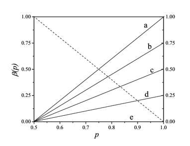
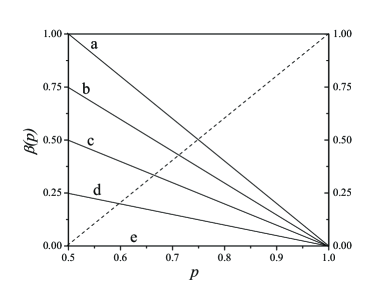
Figure 1: Rational agents: Risk aversion factor $\beta$ as a function of $p$, the probability of favoring the poorer of the two partners. Left panel: The rich agent, solid lines, change its behavior going from rational to irrational (lines a to e). Dash line corresponds to $\beta_{poor}$. Right panel: Here the behavior of the poor agent, solid lines, changes, while the dash line corresponds to $\beta_{rich}$.

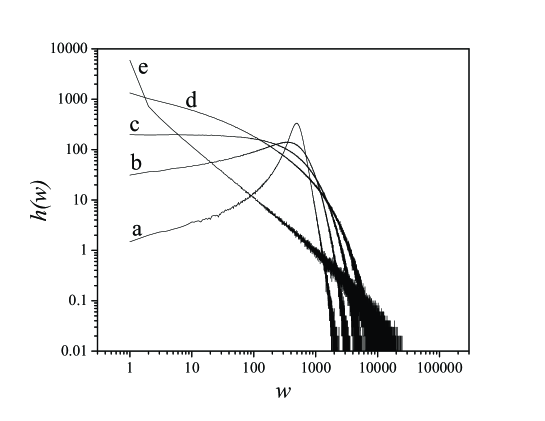
Figure 2: Wealth distribution for the case presented in Fig. 1, right panel, the poor agents change their strategy

In Fig. 2 we have plotted the wealth distribution corresponding for changing strategies of the poorer agent. We have not represented the case when it is the richer agent strategy that changes because we observe that in this case the wealth distribution is independent of the changes and is always equal to the curve (a) of Fig.2. Looking to the (a) curve one observes that a great fraction of the agents concentrate in a middle class with a wealth very near the average value and a few agents have wealth bigger than the initial value of $1000$. This is confirmed by the Gini coefficient of this distribution that is very low, equal to $0.17$. On the other hand, the curves (b) to (e) of Fig. 2 correspond to the case when the risk-aversion of the poorer agents decreases. As it is expected the inequality increases when the poor agents risk more (and there is not a change on the rich side). The number of agents with very low wealth (near $w=1$) increases and for the case where the $\beta$ of the poor partner is $0$ a power law with an exponent approximately equal to the unity is obtained. The Gini coefficients also increase as the risk-aversion of the poor partners decreases as shown in Fig. 5 (open circles), where one can perceive that the Gini coefficients vary almost linearly from $0.17$ to $0.85$.

A different behavior is obtained when the agents behave irrationally. Let’s modify the behaviors described by equation (2), that is, the agents risk more when they have a lower chance to win.

Figure 3: Irrational agents: Risk aversion factor $\beta$ as a function of $p$, the probability of favoring the poorer of the two partners. Left panel: The rich agent, solid lines, changes its behavior (lines a to e). Dash line corresponds to $\beta_{poor}$. Right panel: The poor agent changes its behavior, solid lines. Dash line corresponds to $\beta_{rich}$.

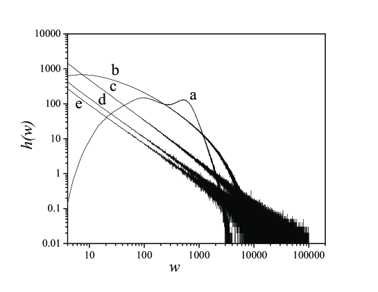
Figure 4: Wealth distribution for the case presented in Fig. 3, left panel, the rich agents change their strategy.

This situation is represented in Fig. 3. If both of them exhibit an “irrational behavior” the effects are mutually neutralized and the distribution of wealth exhibited in the curve Fig. 4(a) has a relatively low Gini coefficient, $\simeq 0.37$. However, if there is a change in the strategy of the richer agents the effects are catastrophic for the poorer partners. This result is shown in curves (b) to (e) of Fig. 4. We can see that the inequality increases very fast, the wealth distribution approaches to a power law with an exponent approximately equal to 1.125 and the Gini coefficients (triangles in Fig. 8) go up to values very near $1.$, i.e. perfect inequality. On the other hand if the poor agents change their strategy there are some minor changes in the wealth distribution, so we have not plotted it. The Gini coefficients are between $0.35$ and $0.4$ (See Fig. 8, squares) with the exception of the last point that corresponds to a zero risk-aversion for the poor partner.

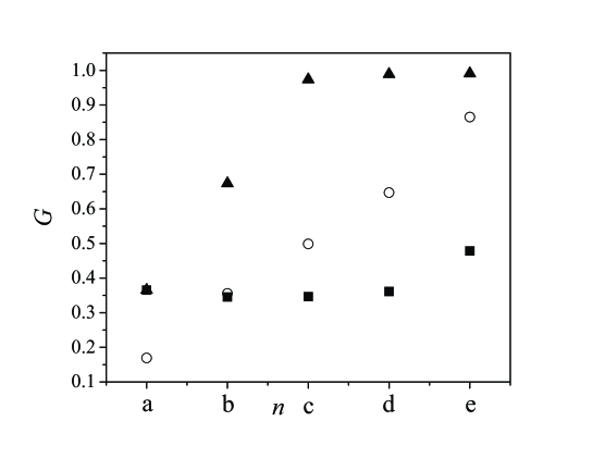
Figure 5: Gini coefficients for rational agents (open circles), and irrational agents when the richer partner changes its strategy(triangles) or the poorer partner changes its strategy (squares)

The results are summarized in Fig. 5 where we have plotted the Gini coefficient in the different situations discussed above. The open circles correspond to the rational behavior when the strategy of the poorer partners changes from the rational to decreasing values of $\beta$ (so, increasing the risk). One can observe an almost linear increase of the inequality. That could mean that when poor agents try to improve their situation risking more, either because of lack of information, or by trying to improve their fortune by betting in high risk speculation, the results are in the opposite direction increasing inequality. On the other hand, in the case of irrational behavior, when there is a change in the strategy of the richer partner (triangles), the Gini coefficient increases very fast up to very high values (near $1$), while if the poorer partner changes its strategy (squares) there are just minor changes in the inequality. In any case if one compares our results with Gini coefficient values for real societies, the values obtained when the rich partner acts “rationally” and the poor partner acts “irrationally” – risking more than reasonable – are closer to empirical data, indicating that either the hypothesis of a previous knowledge of the winning probability is wrong for the poorer partners, either that the poor agents are in a so bad condition that they prefer to risk even in the case of a relatively low winning probability.

References

- (1) Pareto V (1897), Cours d’Economie Politique, Vol. 2, F. Pichou, Lausanne
- (2) Aoyama H, Souma W and Fujiwara Y (2003), Growth and fluctuations of personal and company’s income, Physica A: Statistical Mechanics and its Applications 324:352–358
- (3) Dragulescu A and Yakovenko VM (2000) Statistical Mechanics of Money, The European J. of Physics B 17:723–729
- (4) Dragulescu A and Yakovenko VM (2001) Evidence for the exponential distribution of income in the USA, The European J. of Physics B 20:585–589
- (5) Dragulescu A and Yakovenko VM (2001) Exponential and power-law probability distributions of wealth and income in the United Kingdom and the United States, Physica A: Statistical and Theoretical Physics 299:213–221
- (6) See, for instance, “Econophysics of Wealth Distribution” (Springer-Verlag Italia, 2005), ChatterjeeA , Yarlagadda S and Chakrabarti BK, eds.
- (7) Pianegonda S, Iglesias JR, Abramson G and Vega JL (2003) Wealth redistribution with conservative exchanges Physica A: Statistical and Theoretical Physics 322:667–675
- (8) Iglesias JR, Gonçalves S, Pianegonda S, Vega JL and Abramson G (2003) Wealth redistribution in our small world, Physica A: Statistical and Theoretical Physics 327:12–17
- (9) Pianegonda S and Iglesias JR (2004) Inequalities of wealth distribution in a conservative economy , Physica A: Statistical and Theoretical Physics 42:193–199
- (10) Iglesias JR, Gonçalves S, Abramson G and Vega JL (2004) Correlation between risk aversion and wealth distribution, Physica A: Statistical and Theoretical Physics 342:186–192
- (11) Scafetta N, Picozzi S and West BJ (2002) Pareto’s law: a model of human sharing and creativity cond-mat/0209373v1
- (12) Scafetta N, West BJ and Picozzi S (2003) cond-mat/0209373v1(2002) and A Trade-Investment Model for Distribution of Wealth cond-mat/0306579v2.
- (13) Das A and Yarlagadda S (2005) An analytic treatment of the Gibbs-Pareto behavior in wealth distribution cond-mat 0409329v1 and to be published in Physica A.