An Adaptive Grid Refinement Strategy for the Simulation of Negative Streamers

Abstract

The evolution of negative streamers during electric breakdown of a non-attaching gas can be described by a two-fluid model for electrons and positive ions. It consists of continuity equations for the charged particles including drift, diffusion and reaction in the local electric field, coupled to the Poisson equation for the electric potential. The model generates field enhancement and steep propagating ionization fronts at the tip of growing ionized filaments. An adaptive grid refinement method for the simulation of these structures is presented. It uses finite volume spatial discretizations and explicit time stepping, which allows the decoupling of the grids for the continuity equations from those for the Poisson equation. Standard refinement methods in which the refinement criterion is based on local error monitors fail due to the pulled character of the streamer front that propagates into a linearly unstable state. We present a refinement method which deals with all these features. Tests on one-dimensional streamer fronts as well as on three-dimensional streamers with cylindrical symmetry (hence effectively 2D for numerical purposes) are carried out successfully. Results on fine grids are presented, they show that such an adaptive grid method is needed to capture the streamer characteristics well. This refinement strategy enables us to adequately compute negative streamers in pure gases in the parameter regime where a physical instability appears: branching streamers.

1 Introduction

When non-ionized or lowly ionized matter is exposed to high electric fields, non-equilibrium ionization processes, so-called discharges, occur. They may appear in various forms depending on the spatio-temporal characteristics of the electric field and on the pressure and volume of the medium. One distinguishes the dark, glow or arc discharges that are stationary, and transient non-stationary phenomena such as leaders and streamers. We will focus here on streamers, that are growing filaments of plasma whose dynamics are controlled by highly localized and nonlinear space charge regions.

Streamers occur in nature as well as in many technical applications. They play a role in creating the path of sparks and lightning [1] and they are believed to be directly observable as the multiple channels in so-called sprite discharges. These huge, lightning related discharges above thunderclouds attract large research effort since their first observation in 1989 [2, 3, 4, 5]. Because of the reactive radicals they emit, streamers are used for the treatment of contaminated media like exhaust gasses [6, 7], polluted water [8, 9] or biogas [10]. More recently, efforts have been undertaken to improve the flow around aircraft wings by coupling space charge regions to gas convection [11].

Streamers can be either cathode directed or anode directed; the charge in their head is then positive or negative, respectively. Positive streamers propagate against the drift velocity of electrons, therefore they need additional (and not well known) mechanisms like nonlocal photoionization or background ionization. Negative streamers in simple non-attaching gases like nitrogen or argon, on the other hand, can be described by a minimal model with rather well-accessible parameters [12]. We therefore focus on this case.

The minimal streamer model for negative streamers is a continuum approximation for the densities of the electrons and positive ions with a local field-dependent impact ionization term and with particle diffusion and particle drift in the local electrical field. As space charges of the streamer change the field, and the field determines drift and reaction rates of the particles, the model is nonlinear, and steep ionization fronts between ionized and non-ionized regions emerge dynamically.

After the first claim [13] that a streamer filament within this deterministic continuum model in a sufficiently high field can evolve into an unstable state where it branches spontaneously, streamer branching was observed in more simulations [14, 15, 16]. While the physical nature of the Laplacian instability was elaborated in simplified analytical models [13, 17, 18, 19, 20], other authors challenged the accuracy of the numerical results [21, 22, 23, 24]. Based on purely numerical evidence, their questions were justified, as all simulations within the minimal model up to now were carried out on uniform grids, and the numerical convergence on finer grids could hardly be tested.

Therefore, in the present paper, we present a grid refinement strategy for the minimal streamer model and discuss its results. This procedure allows us to test the numerical convergence of branching, and also to calculate streamers efficiently in longer systems without introducing too many grid points. Moreover, the simulations in [13, 14] were performed on the same uniform grid for both the particle densities and the electric potential. As the Poisson equation for the electric potential has to be solved on the complete large non-ionized outer space, this grid had to be much larger than the actual domain in which the particles evolve. Furthermore, the streamer has an inner layered structure with very steep ionization fronts and thin space charge layers. An efficient refinement is therefore badly needed.

There is an additional complication: standard grid refinement procedures in regions with steep gradients fail due to the pulled character of the streamer front. “Pulling” means that the dynamics and, in particular, the front velocity, is determined in the linearly unstable high field region ahead of the front rather than by the regions with the steepest density gradients [12, 25]. The high field region where any single electron immediately will create an ionization avalanche, is generated by the approaching curved ionization front itself.

In the paper, a refinement strategy dealing efficiently with all these specific problems is developed. It is based on physical insight on the one hand, by which the relevant region for the particle densities can be restricted, and on the knowledge of the importance of the leading edge on the other hand. The drift-diffusion equations for the particle densities and the Poisson equation for the electric potential are treated separately, allowing the solutions for particle densities and electric potential to adapt to the specific difficulties. This refinement procedure will be applied to problems in two spatial dimensions, or in three dimensions with cylindrical symmetry.

The outline of this paper is as follows. First, in Section 2, we give a brief description of the model. In Section 3 the numerical discretizations are introduced and motivated. Section 4 discusses the refinement procedure. Section 5 contains a one-dimensional example in which some of the essential numerical difficulties with local grid refinements of pulled fronts are illustrated and discussed. Section 6 deals with the performance of our refinement algorithm, and the results are presented in the Section 7. The final section contains a discussion of the results and conclusions.

2 Hydrodynamic approximation for the ionized channel

2.1 Drift, diffusion and ionization in a gas

The essential properties of anode directed streamer propagation in a non-attaching gas like $N_{2}$ or $Ar$, can be analyzed by a fluid model for two species of charged particles (electrons and positive ions). It consists of continuity equations for the electron and positive ion number densities, $n_{e}$ and $n_{+}$,

$$\displaystyle\frac{\partial n_{e}}{\partial t} -\nabla\cdot(n_{e}\mu_{e}{\bf E}+D_{e}\nabla n_{e}) =S_{i}\,,$$ (2.1)

$$\displaystyle\frac{\partial n_{+}}{\partial t} =S_{i}\,.$$ (2.2)

The electrons drift with a velocity $\mu_{e}{\bf E}$ and diffuse with a diffusion coefficient $D_{e}$. Here ${\bf E}$ is the local electric field and $\mu_{e}$ the electron mobility. The ions can be considered to be immobile on the short time scales considered here, since their mobility is two orders of magnitude smaller than that of the electrons [26]. We remark that extending our algorithm to moving ions and eventually other species is rather straightforward, and not including this makes no difference for the algorithm itself.

The source term $S_{i}$ represents creation of electrons and positive ions through impact ionization, and is the same for both species since charge is conserved during an ionization event. The impact ionization can be described with Townsend’s approximation [27] (but any other local field dependence can be inserted as well)

$$S_{i}=n_{e}\mu_{e}|{\bf E}|\alpha(|{\bf E}|)=n_{e}\mu_{e}|{\bf E}|\alpha_{0}\,e^{-E_{0}/|{\bf E}|}\,,$$ (2.3)

where $\alpha_{0}$ is the ionization coefficient and $E_{0}$ the threshold field for ionization. We do not include photoionization or recombination since, in the particular case of $N_{2}$ and for the short time scales considered, these processes are negligible compared to impact ionization [22]. However, an ionization mechanism such as photoionization is essential for the development of positive streamers, which are therefore excluded from the present study.

The electric field ${\bf E}$ is determined through Poisson’s equation for the electric potential $V$,

$$\nabla^{2}V=\frac{e}{\epsilon_{0}}(n_{e}-n_{+})\,,\,\,\,\,\,\,{\bf E}=-\nabla V\,,$$ (2.4)

where $\epsilon_{0}$ is the permittivity of free space, and $e$ the electron charge.

2.2 Dimensional analysis

This model has been implemented in dimensionless form. The characteristic length and field scales emerge directly from Townsend’s ionization formula (2.3) as $l_{0}=\alpha_{0}^{-1}$ and $E_{0}$, respectively. The characteristic velocity is then given as $v_{0}=\mu_{e}E_{0}$, which leads to a characteristic timescale $t_{0}=l_{0}/v_{0}=l_{0}/(\mu_{e}E_{0})$. The characteristic diffusion coefficient then becomes $D_{0}=l_{0}^{2}/t_{0}$. The number density scale emerges from the Poisson equation (2.4), $n_{0}=\epsilon_{0}E_{0}/el_{0}$. We use the values from [26, 28] for $\mu_{e}$, $E_{0}$ and $\alpha_{0}$ in $N_{2}$ at 300 K, which depend on the neutral gas density,

$$\mu_{e}\simeq\frac{380}{(N/N_{0})}\,\,\,\frac{{\rm cm^{2}}}{{\rm V\,s}}\,,\,\,\alpha_{0}\simeq\frac{4332}{(N/N_{0})}\,\,\,\frac{1}{\rm cm}\,,\,\,E_{0}\simeq\frac{2\cdot 10^{5}}{(N/N_{0})}\,\,\,\frac{\rm V}{\rm cm}\,.$$ (2.5)

Inserting these values in the characteristic scales we obtain, for molecular nitrogen at normal conditions,

$$\displaystyle l_{0}\simeq\frac{2.3\cdot 10^{-4}}{(N/N_{0})}\,\,\,{\rm cm}\,,\,\,\,\,\,\,\displaystyle t_{0}\simeq\frac{3\cdot 10^{-12}}{(N/N_{0})}\,\,\,{\rm s}\,,\,\,\,\,\,\,\displaystyle n_{0}\simeq\frac{4.7\cdot 10^{14}}{e\,((N/N_{0})^{2}}\,\,\,\frac{1}{\rm cm^{3}}\,,\,\,\,\,\,\,\displaystyle D_{0}\simeq\frac{1.8\cdot 10^{4}}{(T/T_{0})}\,\,\,\frac{\rm cm^{2}}{\rm s}\,.$$ (2.6)

Here $N_{0}$ and $T_{0}$ are the neutral gas density and temperature under normal conditions. The dimensionless quantities are then defined as follows,

$$\displaystyle{\bf r}=\frac{{\bf R}}{l_{0}}\,,\,\,\,\,\,\,\displaystyle\tau=\frac{t}{t_{0}}\,,\,\,\,\,\,\,\displaystyle\sigma=\frac{n_{e}}{n_{0}}\,,\,\,\,\,\,\,\displaystyle\rho=\frac{n_{+}}{n_{0}}\,,\,\,\,\,\,\,\displaystyle{\boldsymbol{\mathcal{E}}}=\frac{{\bf E}}{E_{0}}\,,\,\,\,\,\,\,\displaystyle\phi=\frac{V}{(E_{0}l_{0})}\,,\,\,\,\,\,\,\displaystyle D=\frac{D_{e}}{D_{0}}\,.$$ (2.7)

For the diffusion coefficient we use the value given in [29], $D_{e}$=1800 cm² s^-1, which gives a dimensionless diffusion coefficient of 0.1 under normal conditions.

Inserting these dimensionless quantities into the continuity equations (2.1)-(2.4), we obtain

$$\displaystyle\frac{\partial\sigma}{\partial\tau} = \nabla\cdot(\sigma{\boldsymbol{\mathcal{E}}}+D\nabla\sigma)+\sigma|{\boldsymbol{\mathcal{E}}}|\exp(-1/|{\boldsymbol{\mathcal{E}}}|)\,,$$ (2.8)

$$\displaystyle\frac{\partial\rho}{\partial\tau} = \sigma|{\boldsymbol{\mathcal{E}}}|\exp(-1/|{\boldsymbol{\mathcal{E}}}|)\,,$$ (2.9)

$$\displaystyle\nabla^{2}\phi = \sigma-\rho\,,\quad{\boldsymbol{\mathcal{E}}}=-\nabla\phi\,,$$ (2.10)

where $\sigma$ and $\rho$ denote the dimensionless electron and ion number densities, respectively, $\tau$ the dimensionless time, ${\boldsymbol{\mathcal{E}}}$ the dimensionless electric field, $\phi$ the dimensionless electric potential and $D$ the dimensionless diffusion coefficient.

We refer to the equations (2.8)-(2.10) as the minimal streamer model, since it contains all the basic physics needed for negative streamers in a non-attaching gas.

2.3 Geometry and boundary conditions

In narrow geometries, streamers frequently are growing from pointed electrodes, that create strong local fields in their neighborhood and a pronounced asymmetry between the initiation of positive and negative streamers [30]. On the other hand, in many natural discharges and, in particular, for sprites above thunderclouds [15], it is appropriate to assume that the electric field is homogeneous. Of course, dust particles or other nucleation centers can play an additional role in discharge generation, but in this paper we will focus on the effect of a homogeneous field on a homogeneous gas.

The computational domain is limited by two planar electrodes. The model is implemented in a cylindrical symmetric coordinate system $(r,z)\in(0,L_{r})\times(0,L_{z})$, such that the electrodes are placed perpendicular to the axis of symmetry ($r$=0), the cathode at $z=0$ and the anode at $z=L_{z}$. The boundary conditions for the electric potential read

$$\phi(r,0,\tau)=0\,,\qquad\phi(r,L_{z},\tau)=\phi_{0}>0\,,\qquad\frac{\partial\phi}{\partial r}(L_{r},z,\tau)=0\,.$$ (2.11)

The background electric field then becomes

$${{\boldsymbol{\mathcal{E}}}_{b}}=-|{\boldsymbol{\mathcal{E}}}_{b}|{\bf\hat{e}_{z}}=-\frac{\phi_{0}}{L_{z}}{\bf\hat{e}_{z}}\,,$$ (2.12)

where ${\bf\hat{e}_{z}}$ is the unit vector in the $z-$direction. The radial boundary at $L_{r}$ is virtual, and only present to create a finite computational domain. In order for the boundary condition no to affect the solution near the axis of symmetry along which the streamer propagates, we need to place this boundary relatively far from the axis of symmetry.

Throughout this article, we use a Gaussian initial ionization seed, placed on the axis of symmetry, at a distance $z=z_{b}$ from the cathode,

$$\sigma(r,z,0)=\rho(r,z,0)=\sigma_{0}\exp\left(\frac{r^{2}+(z-z_{b})^{2}}{R_{b}^{2}}\right)\,.$$ (2.13)

The maximal density $\sigma_{0}$ of this seed, the radius $R_{b}$ at which the density drops to 1/e of its maximal value, and the value of $z_{b}$ differ from case to case, and will be specified where needed. Furthermore, the use of a dense seed, in particular in low fields, accelerates the emergence of a streamer. We remark that the initial seed is charge neutral.

The continuity equation for the electron density is second order in space, and therefore requires two boundary conditions for each direction in space. At $r=L_{r}$ and $z=L_{z}$ we use Neumann boundary conditions, so that electrons that arrive at those boundaries may flow out of or into the system, but in all cases discussed in this paper the streamer is too far from the boundary for this to happen. At the cathode, we impose either homogeneous Neumann or Dirichlet boundary conditions. In the first case we again allow for a net flux of particles through the boundary. Dirichlet conditions will only be used for a one-dimensional test in this paper. To recapitulate, the boundary conditions for the electrons read

$$\frac{\partial\sigma}{\partial z}(r,0,\tau)=0\,,\text{ or }\sigma(r,0,\tau)=0\,,\quad\frac{\partial\sigma}{\partial z}(r,L_{z},\tau)=0\,,\quad\frac{\partial\sigma}{\partial r}(L_{r},z,\tau)=0\,.$$ (2.14)

We notice that, if $z_{b}\gg R_{b}$, the ionization seed is detached from the cathode, and this results in practice in a zero inflow of electrons. On the other hand, placing the seed near the cathode will result in an inflow of electrons. Varying the value of $z_{b}$ will therefore enable us to investigate the influence of the inflow of electrons on the streamer propagation.

3 Numerical discretizations

In our numerical simulations we shall mainly consider the streamer model with radial symmetry, making it effectively two dimensional. To illustrate some of the difficulties and their solutions we will also deal with the one-dimensional case.

In the cylindrically symmetric coordinate system introduced in the previous section, the equations (2.8)-(2.10) read

$$\frac{\partial\sigma}{\partial\tau} = \displaystyle\frac{1}{r}\frac{\partial(r\sigma{\mathcal{E}}_{r})}{\partial r}+\frac{\partial(\sigma{\mathcal{E}}_{z})}{\partial z}+\frac{D}{r}\frac{\partial}{\partial r}(r\frac{\partial\sigma}{\partial r})+D\frac{\partial^{2}\sigma}{\partial z^{2}}+\sigma|{{\boldsymbol{\mathcal{E}}}}|e^{-1/|{{\boldsymbol{\mathcal{E}}}}|}\,,$$ (3.1)

$$\displaystyle\frac{\partial\rho}{\partial\tau} = \displaystyle\sigma|{{\boldsymbol{\mathcal{E}}}}|e^{-1/|{{\boldsymbol{\mathcal{E}}}}|}\,,$$ (3.2)

$$\displaystyle\nabla^{2}\phi = \displaystyle\frac{1}{r}\frac{\partial}{\partial r}(r\frac{\partial\phi}{\partial r})+\frac{\partial^{2}\phi}{\partial z^{2}}\;=\;\sigma-\rho\,.$$ (3.3)

The electric field ${{\boldsymbol{\mathcal{E}}}}=({\mathcal{E}}_{r},{\mathcal{E}}_{z})^{\text{T}}$ can be computed from the electric potential as

$${{\boldsymbol{\mathcal{E}}}}=-\nabla\phi=-\Big{(}\frac{\partial\phi}{\partial r},\,\frac{\partial\phi}{\partial z}\Big{)}^{\rm T}\,.$$ (3.4)

The boundary conditions for this system have been treated in Sect. 2.3.

3.1 Spatial discretization of the continuity equations

The equations will be solved on a sequence of (locally) uniform grids with cells

$${\mathcal{C}}_{ij}=[(i-1)\Delta r,i\Delta r]\times[(j-1)\Delta z,j\Delta z],\,i=1...M_{r},\,j=1...M_{z}\,,$$

where $M_{r}=L_{r}/\Delta r$ and $M_{z}=L_{z}/\Delta z$ are the number of grid points in the $r$- respectively $z$-direction, and cell centers $(r_{i},z_{j})=((i-\frac{1}{2})\Delta r,(j-\frac{1}{2})\Delta z)$. We denote by $\sigma_{i,j}$ and $\rho_{i,j}$ the density approximations in the cell centers. These can also be viewed as cell averages. The electric potential $\phi_{ij}$ and field strength $|{{\boldsymbol{\mathcal{E}}}}|_{i,j}$ are taken in the cell centers, whereas the electric field components are taken on the cell vertices. For the moment it is supposed that the electric field is known, its computation will be discussed later on.

The equations for the particle densities are discretized with finite volume methods, based on mass balances for all cells. Rewriting the continuity equations (3.1)-(3.2) will result in the semi-discrete system

$$\begin{array}[]{rcl}\displaystyle\frac{d\sigma_{i,j}}{d\tau}&=&\displaystyle\frac{1}{r_{i}\Delta r}(r_{i-\frac{1}{2}}F_{i-\frac{1}{2},j}-r_{i+\frac{1}{2}}F_{i+\frac{1}{2},j})+\frac{1}{\Delta z}(F_{i,j-\frac{1}{2}}-F_{i,j+\frac{1}{2}})+S_{i,j}\,,\\[11.38109pt] \displaystyle\frac{d\rho{{}_{i,j}}}{d\tau}&=&\displaystyle S_{i,j}\,,\end{array}$$ (3.7)

in which $F=F^{a}+F^{d}$. $F^{a}$ and $F^{d}$ are the advective and diffusive electron fluxes through the cell boundaries, and $S_{ij}$ is the source term in the grid cell ${\mathcal{C}}_{ij}$.

The discretization of the advective terms requires care. A first order upwind scheme as used in [22, 24] appears to be much too diffusive [31], leading to a totally different asymptotic behavior on realistic grids. Moreover, it is expected that the numerical diffusion might over-stabilize the numerical scheme, thereby suppressing interesting features of the solutions. This explains why streamer branching is not seen by the authors of [22, 24]. On the other hand, higher order linear discretizations lead to numerical oscillations and negative values for the electron density, that will grow in time due to the reaction term. This holds in particular for central discretizations [32]. The choice was made to use an upwind-biased scheme with flux limiting. This gives mass conservation and monotone solutions without introducing too much numerical diffusion. For the limiter we will take the Koren limiter function, which is slightly more accurate than standard choices such as the van Leer limiter function [32].

Denoting $v^{+}=\max(v,0)$ and $v^{-}=\min(v,0)$ to distinguish upwind directions for the components of the drift velocity $v_{r}=-{\mathcal{E}}_{r}$ and $v_{z}=-{\mathcal{E}}_{z}$, the advective fluxes in the $r$- direction are computed by

$$F^{a}_{i+\frac{1}{2},j}=v^{+}_{r;\,i+\frac{1}{2},j}\Big{[}\sigma_{i,j}+\psi\big{(}\theta_{i,j}\big{)}\big{(}\sigma_{i+1,j}-\sigma_{i,j}\big{)}\Big{]}+\,v^{-}_{r;\,i+\frac{1}{2},j}\Big{[}\sigma_{i+1,j}+\psi\big{(}\frac{1}{\theta_{i+1,j}}\big{)}\big{(}\sigma_{i,j}-\sigma_{i+1,j}\big{)}\Big{]},$$ (3.8)

in which

$$\theta_{i,j}=\frac{\sigma_{i,j}-\sigma_{i-1,j}}{\sigma_{i+1,j}-\sigma_{i,j}}\,,\qquad\psi(\theta)=\max\Big{(}0,\min\Big{(}1,\frac{1}{3}+\frac{\theta}{6},\theta\Big{)}\Big{)}\,.$$ (3.9)

The advective fluxes in the vertical direction are computed in the same way; the fact that the $r$-direction is radial is already taken care of in (3.7). Note that in regions where the solution is smooth we will have values of $\theta_{ij}$ close to $1$, and then the scheme simply reduces to the third-order upwind-biased discretization corresponding to $\psi(\theta)=\frac{1}{3}+\frac{1}{6}\theta$. In non-smooth regions where monotonicity is important the scheme can switch to first-order upwind, which corresponds to $\psi(\theta)=0$.

The diffusive fluxes are calculated with standard second-order central differences as

$$F^{d}_{i+\frac{1}{2},j}=\frac{D}{\Delta r}(\sigma_{i,j}-\sigma_{i+1,j})\,.\qquad F^{d}_{i,j+\frac{1}{2}}=\frac{D}{\Delta z}(\sigma_{i,j}-\sigma_{i,j+1})\,,$$ (3.10)

Finally, the reaction term $S_{ij}$ in (3.7) is computed in the cell centers as

$$S_{i,j}=\sigma_{i,j}|{{\boldsymbol{\mathcal{E}}}}|_{ij}e^{-1/|{{\boldsymbol{\mathcal{E}}}}|_{ij}}\,.$$ (3.11)

Boundary values will be either homogeneous Dirichlet or homogeneous Neumann type. For example, for Dirichlet boundary conditions $\sigma=0$ for $z=0$, we introduce virtual values [32]

$$\sigma_{i,0}=-\sigma_{i,1}\,,\quad\sigma_{i,-1}=-\sigma_{i,2}\,.$$ (3.12)

For Neumann boundary conditions $\partial_{z}\sigma=0$ for $z=0$ we set

$$\sigma_{i,0}=\sigma_{i,1}\,,\quad\sigma_{i,-1}=\sigma_{i,2}\,.$$ (3.13)

These formulas follow from the approximations

$$\begin{array}[]{rcl}\sigma(r_{i},z_{\frac{1}{2}})&=&\displaystyle\frac{1}{2}(\sigma(r_{i},z_{0})+\sigma(r_{i},z_{1}))+\mathcal{O}(\Delta z^{2})\\ \sigma_{z}(r_{i},z_{\frac{1}{2}})&=&\displaystyle\frac{1}{\Delta z}(\sigma(r_{i},z_{1})-\sigma(r_{i},z_{0}))+\mathcal{O}(\Delta z^{2})\end{array}$$ (3.16)

3.2 Spatial discretization of the Poisson equation

The electric potential $\phi$ is computed through a second-order central approximation of Eq. (2.10), and is defined at the cell centers:

$$\sigma_{i,j}-\rho_{i,j}=\displaystyle\frac{\phi_{i+1,j}-2\phi_{i,j}+\phi_{i-1,j}}{\Delta r^{2}}+\frac{\phi_{i+1,j}-\phi_{i-1,j}}{2r_{i}\Delta r} \,\,\,+ \displaystyle\frac{\phi_{i,j+1}-2\phi_{i,j}+\phi_{i,j-1}}{\Delta z^{2}}\,.$$ (3.17)

The electric field components are then computed by using a second-order central discretization of ${{\boldsymbol{\mathcal{E}}}}=-\nabla\phi$, they are defined in the cell boundaries,

$${\mathcal{E}}_{r;i+\frac{1}{2},j}=\frac{\phi_{i,j}-\phi_{i+1,j}}{\Delta r}\,,\qquad{\mathcal{E}}_{z;i,j+\frac{1}{2}}=\frac{\phi_{i,j}-\phi_{i,j+1}}{\Delta z}\,.$$ (3.18)

The electric field strength is computed at the cell centers, therefore the components are first determined in the cell centers by averaging the cell boundary values, and the electric field strength then becomes:

$$|{{\boldsymbol{\mathcal{E}}}}|_{i,j}=\frac{1}{2}\sqrt{({\mathcal{E}}_{r;i-\frac{1}{2},j}+{\mathcal{E}}_{r;i+\frac{1}{2},j})^{2}+({\mathcal{E}}_{z;i,j-\frac{1}{2}}+{\mathcal{E}}_{z;i,j+\frac{1}{2}})^{2}}\,.$$ (3.19)

We notice here that, discretizing $\nabla\cdot{{\boldsymbol{\mathcal{E}}}}$ with a second-order central scheme gives

$$\frac{\partial}{\partial\tau}(\nabla\cdot{{\boldsymbol{\mathcal{E}}}})=\frac{\partial(\sigma_{i,j}-\rho_{i,j})}{\partial\tau}\,.$$

Therefore, the total current conservation,

$$\nabla\cdot\left(\frac{\partial{{\boldsymbol{\mathcal{E}}}}}{\partial\tau}+\sigma{\boldsymbol{\mathcal{E}}}+D\nabla\sigma\right)=0\,,$$ (3.20)

also holds on the level of the discretizations.

3.3 Temporal discretization

After the spatial discretization, the system of equations (3.7) can be written in vector form as a system of ordinary differential equations,

$$\begin{array}[]{lcr}\displaystyle\frac{d\sigma}{d\tau}&=&G(\sigma,{{\boldsymbol{\mathcal{E}}}})\,,\\[11.38109pt] \displaystyle\frac{d\rho}{d\tau}&=&S(\sigma,{{\boldsymbol{\mathcal{E}}}})\,,\end{array}$$ (3.23)

where the components of $G$ and $S$ are given by the spatial discretizations in (3.7). The electric field ${{\boldsymbol{\mathcal{E}}}}$ and the field strength $|{{\boldsymbol{\mathcal{E}}}}|$ are computed from given $\sigma,\rho$ by discretized versions of (3.3) and (3.4), discussed in Sect. 4.4. Therefore the full set of semi-discrete equations actually forms a system of differential-algebraic equations.

The particle densities are updated in time using the explicit trapezoidal rule, which is a two-stage method, with step size $\Delta\tau$. Starting at time $\tau^{n}=n\Delta\tau$ from known particle distributions $\sigma^{n}(r,z)\approx\sigma(r,z,\tau^{n})$, $\rho^{n}(r,z)\approx\rho(r,z,\tau^{n})$ and known electric field ${{\boldsymbol{\mathcal{E}}}}^{n}(r,z)\approx{{\boldsymbol{\mathcal{E}}}}(r,z,\tau^{n})$, the predictors $\bar{\sigma}^{n+1}$ and $\bar{\rho}^{n+1}$ for the electron and ion densities at time $\tau^{n+1}$ are first computed by

$$\begin{array}[]{l}\displaystyle\bar{\sigma}^{n+1}\;=\;\sigma^{n}+\Delta\tau\,G(\sigma^{n},{{\boldsymbol{\mathcal{E}}}}^{n})\,,\\[11.38109pt] \displaystyle\bar{\rho}^{n+1}\;=\;\rho^{n}+\Delta\tau\,S(\sigma^{n},{{\boldsymbol{\mathcal{E}}}}^{n})\,,\end{array}$$ (3.26)

After this the Poisson equation (3.3) is solved with source term $\bar{\sigma}^{n+1}-\bar{\rho}^{n+1}$, leading to the electric field $\bar{{\boldsymbol{\mathcal{E}}}}^{n+1}$ at this intermediate stage by Eq. (3.4). The final densities at the new time level $\tau^{n+1}$ are then computed as

$$\begin{array}[]{l}\displaystyle\sigma^{n+1}\;=\;\sigma^{n}+\frac{\Delta\tau}{2}G(\sigma^{n},{{\boldsymbol{\mathcal{E}}}}^{n})+\frac{\Delta\tau}{2}G(\bar{\sigma}^{n+1},\bar{{\boldsymbol{\mathcal{E}}}}^{n+1})\,,\\[11.38109pt] \displaystyle\rho^{n+1}\;=\;\rho^{n}+\frac{\Delta\tau}{2}S(\sigma^{n},{{\boldsymbol{\mathcal{E}}}}^{n})+\frac{\Delta\tau}{2}S(\bar{\sigma}^{n+1},\bar{{\boldsymbol{\mathcal{E}}}}^{n+1})\,,\end{array}$$ (3.29)

after which the Poisson equation is solved once more, but now with the source term $\sigma^{n+1}-\rho^{n+1}$, giving the electric field ${{\boldsymbol{\mathcal{E}}}}^{n+1}$ induced by the final particle densities at time $\tau^{n+1}$. This time discretization is second-order accurate, which is in line with the accuracy of the spatial discretization.

The use of an explicit time integration scheme implies that the grid spacing and time step should obey restrictions for stability. For the advection part we get a Courant-Friedrichs-Lewy (CFL) restriction

$$\displaystyle\max{\mathcal{E}}_{r}\frac{\Delta\tau}{\Delta r}+\max{\mathcal{E}}_{z}\frac{\Delta\tau}{\Delta z} < \nu_{a}\,,$$ (3.30)

and the diffusion part leads to

$$\displaystyle D\frac{\Delta\tau}{\Delta r^{2}}+D\frac{\Delta\tau}{\Delta z^{2}} < \nu_{d}\,.$$ (3.31)

Actually, to be more precise, a combination of (3.30), (3.31) should be considered. However, in our simulations, condition (3.30) will dominate and the time step will be chosen well inside this constraint.

For the first order upwind advection scheme combined with a two-stage Runge-Kutta method, the maximal Courant number is [32] $\nu_{a}^{1}=1$, while for the third order upwind scheme it is $\nu_{a}^{3}=0.87$. The second order central discretization demands a maximal Courant number $\nu_{d}=0.5$.

A third restriction for the time step comes from the dielectric relaxation time. The ions are considered to be immobile, which leaves us with the following time step restriction in dimensional units [33],

$$\Delta t\leq\frac{\epsilon_{0}}{e\mu_{e}\max n_{e}}\,,$$ (3.32)

where we refer to the previous section for the meaning of these quantities. If we apply the dimensional analysis of the previous section, we obtain the time step restriction in dimensionless units,

$$\Delta\tau\leq\frac{1}{\sigma}\,.$$ (3.33)

In practice, it appears that this restriction is much weaker than that for the stability of the numerical scheme.

The choice for an explicit time stepping scheme was made after tests with VLUGR [34], a local refinement code that uses –computationally much more intensive– implicit schemes (BDF2). These tests showed that these implicit schemes also needed relatively small time steps to obtain accurate solutions, so that in the end an explicit scheme would be more efficient in spite of stability restrictions for the time steps. Moreover the use of an explicit scheme allows us to decouple the computation of the particle densities from that of the electric potential and electric fields. With a fully implicit scheme all quantities are coupled, leading to much more complex computations and longer computation times.

Another reason for preferring explicit time stepping is monotonicity. The solutions in our model have very steep gradients for which we use spatial discretizations with limiters to prevent spurious oscillations. Of course, such oscillations should also be prevented in the time integration. This has led to the development of schemes with TVD (total variation diminishing) or SSP (strong stability preserving) properties; see [35, 32]. In contrast to stability in the von Neumann sense (i.e., $L_{2}$-stability for linear(ized) problems with (frozen) constant coefficients), such monotonicity requirements do not allow large step sizes with implicit methods of order larger than one. Among the explicit methods, the explicit trapezoidal rule is optimal with respect to such monotonicity requirements.

3.4 Remarks on alternative discretizations

The above combination of spatial and temporal discretizations provide a relatively simple scheme for the streamer simulations. The accuracy will be roughly $O(\Delta x^{2})+O(\Delta\tau^{2})$ in regions where the solution is smooth (also for the limited advection discretization [32, p. 218]). In our tests, step size restrictions mainly originate from the advective parts in the continuity equations. The above scheme is stable and monotone (free of oscillations) for Courant numbers up to one, approximately. Usually we take smaller step sizes than imposed by this bound to reduce temporal errors.

As mentioned before in Sect. 3.1 using a first-order upwind discretization for the advective term will usually give rise to too much diffusion, whereas second-order central advection discretizations lead to numerical oscillations and negative concentrations.

Higher-order discretizations can certainly be viable alternatives. However, we then will have larger spatial stencils, which creates more difficulties with local grid refinements where numerical interfaces are created. The above discretization is robust and easy to implement.

It is well known that limiting as in (3.8) gives some clipping of peak values in linear advection tests, simply because the limiter does not distinguish genuine extrema from oscillations induced numerically. This can be avoided by adjusting the limiter near extrema, but in the streamer tests it was found that such adjustments were not necessary. In the streamer model the local extrema in each spatial direction are located in the streamer head, and the nonlinear character of the equations gives a natural steepening there which counteracts local numerical dissipation.

In [28] a flux-corrected transport (FCT) scheme was used. The advantage of our semi-discrete approach is that is becomes easier to add source terms without having to change the simulation drastically. Also the transition from 1D discretizations to 2D or 3D becomes straightforward conceptually; the implementations for higher dimensions are still difficult, of course, in particular for the Poisson equation. Moreover, in [31] comparisons of the FCT scheme with a scheme using the van Leer limiter (which is closely related to the limiter used in our scheme) show that the FCT scheme, in contrast to the limited scheme, gives somewhat irregular results for simple advection tests in regions with small densities. In the leading edge the densities decay exponentially, and we do not want such irregularities to occur.

4 The adaptive refinement procedure

4.1 The limitations of the uniform grid approach

Up to now, all simulations that have been carried out on the minimal streamer model were performed on a uniform grid [26, 28, 13, 14]. However the use of a uniform grid on such a large system has several limitations.

The first limitation is the size of the system. In [13, 14] the simulations were performed in a radially symmetric geometry with $2000\times 2000=4\cdot 10^{6}$ grid points. Since the number of variables is of at least 10 per grid point (the electron and ion densities both at old and new time step, the electric potential, the electric field components and strength, and the terms containing the temporal derivatives of both electrons and ions), the total number of variables will be at least $40\cdot 10^{6}$. So, when computing in double precision (64 bits or 8-bytes values) the memory usage is in the order of several hundreds MB, depending on the compiler. Moreover, these simulations show that the streamer will eventually branch, and up to now there was no convergence of the branching time with respect to the mesh size. In order to investigate the branching, it would be necessary to rerun the simulation with a smaller grid size. Moreover it would be interesting to investigate larger systems. So from that point of view it is worth looking at an algorithm that would require much less memory usage.

The second limitation comes from the Poisson equation, which has to be solved at each time step, and therefore requires a fast solver. For this we use the Fishpak routine, described in [36, 37]. One of the major limitations of this routine is its ineptitude to deal accurately with very large grids, due to numerical instabilities with respect to round-off errors. Numerical experiments show that on an $m_{r}\times m_{z}$ grid with either $m_{r}$ or $m_{z}$ substantially larger than 2000, the Fishpak routine gives large errors due to numerical instabilities with respect to round-off errors. An illustration is presented in the appendix.

It is necessary to develop some strategy to counteract these limitations. This will be done by choosing separate grids with suitable local refinements for the continuity equations (2.8)-(2.9) and the Poisson equation (2.10).

4.2 General structure of the locally uniform refined grids

Both the continuity equations (3.1) and the Poisson equation (3.3) are computed on a set of uniform, radially symmetric grids, that are refined locally where needed. Solving these equations separately rather than simultaneously allows the use of different sets of grids for each equation, thereby making it possible to decouple the grids for the continuity equation from those of the Poisson equation; grids can then be tailored for the particular task at hand. We emphasize that it is the use of an explicit time stepping method that allows us to decouple the grids.

In both cases the equations are first solved on a coarse grid. This grid is then refined in those regions where a refinement criterion – which will be treated in more detail below – is met. These finer grids can be further refined, wherever the criterion is still satisfied. Both the grids and the refinement criteria may be different for the continuity equations on the one hand and the Poisson equation on the other hand, but the general structure of the grids is the same for both type of equations. It consists of a series of nested grids $\Omega^{k}$, $k$ being the grid number, with level $l(k)$. This level function gives the mesh width of a grid, $l(1)=1$ corresponding to the coarsest grid $\Omega^{1}$ with mesh width $\Delta r^{c}$ and $\Delta z^{c}$. A certain grid will have a mesh twice as fine as the grid one level coarser – which we will call its parent grid – so that the mesh widths of a grid with level $l$ become $\Delta r^{l}={\Delta r^{c}}/{2^{l-1}}$ and $\Delta z^{l}={\Delta z^{c}}/{2^{l-1}}$.

Fig. 1 shows an example of four nested grids on three levels. We will denote a quantity $u$ on a certain grid $\Omega^{k}$ with level $l=l(k)$ as $u^{k}_{ij}=u(r^{l}_{i},z^{l}_{j})$. All grids are characterized by the coordinates of their corners relative to the origin of the system (on the axis of symmetry at the cathode), so that $r_{i}^{l}=(i-1/2)\Delta r^{l}$, $z_{j}^{l}=(j-1/2)\Delta z^{l}$.

Figure 1: An example of nested grids: $\scriptscriptstyle\blacksquare$ cell centers on $\Omega^{1}$ with $l(1)=1$, $\times$ cell centers on $\Omega^{2}$ with $l(2)=2$, $+$ cell centers on $\Omega^{3}$ with $l(3)=3$, $\circ$ cell centers on $\Omega^{4}$ with $l(4)=3$.

Throughout this article, the grids for the Poisson equation are denoted by $\mathcal{G}$, those for the continuity equations by $\mathcal{H}$. For the continuity equations, the grids are structured as follows: we determine all grid cells of a grid $\mathcal{H}^{l}$ at a certain level $l$ that, following some refinement monitor (we will give more details later), have to be refined. This results in one or more sets of connected finer grid cells. As a first step, we chose the finer child grids $\{\mathcal{H}^{l+1}\}$ of the parent grid $\mathcal{H}^{l}$ to cover the smallest rectangular domain enclosing each of these sets of connected grid cells. Although this first rudimentary approach gave some gain in computational time, it lead to a large number of unnecessary fine grid cells, due to the curved nature of the ionization front. So instead, we divide such unnecessary large rectangles into smaller rectangular patches, thereby limiting the number of fine grid cells. Obviously, the union of all these child grids $\{\mathcal{H}^{l+1}\}$ should contain all the grid cells indicated by the monitor. For programming reasons, the rectangular child grids $\{\mathcal{H}^{l+1}\}$ were chosen to all have an equal, arbitrary number $M_{0}$ of grid points in the radial direction. Using a large value for $M_{0}$ leads to unnecessary large child grids, using a small value would make no sense because each grid requires the storage of boundary values. Since the rectangular grid structure is preserved, this could be relatively easily be implemented in the existing code, and using a suitable value of $M_{0}$ lead to a significant gain in computational time and memory.

To compute the electric potential, however, such a grid distribution is not appropriate. This comes from our use of a fast Poisson solver, which computes, on a rectangular grid, the potential induced by a space charge distribution on that same rectangular grid. The solution of the Poisson equation is not, however, determined locally, and these non local effects are not accounted for properly if we compute the potential on smaller rectangles like the continuity equation. So in the case of the Poisson equation we use the same grid structure as we first did for the continuity equation: we determine, using some refinement monitor, all grid cells of a grid $\mathcal{G}^{l}$ at a certain level $l$ that have to be refined, and the finer child grid $\{\mathcal{G}^{l+1}\}$ of the parent grid $\mathcal{G}^{l}$ is set to cover the smallest rectangular domain enclosing all these grid cells.

In what follows, to make the distinction between the indices on a coarse and on a fine grid, we use capital indices $I$ and $J$ for the coarse grid and small indices $i$ and $j$ for the fine grid. Notice that a coarse grid cell with the cell center $(r_{I},z_{J})$ contains four finer cells with centers $(r_{i},z_{j})$, $(r_{i},z_{j+1})$, $(r_{i+1},z_{j})$, $(r_{i+1},z_{j+1})$, with $i=2I-1$ and $j=2J-1$.

Let us now discuss in more details the refinement algorithm for the continuity equations and that for the Poisson equation, and the benefits of decoupling the grids for both equations.

4.3 Refinement scheme for the continuity equation

Let us assume that the particle distributions and electric field at time $\tau^{n}$ are known on a set $S^{n}$ of $m$ rectangular grids $\mathcal{H}^{n,k}$ with level $l=l(k)$, $1\leq k\leq m$, as shown in Fig. 2.

Then, using the explicit time stepping method introduced in Sect. 3.3, the particle distributions at time $\tau^{n+1}$ can be computed on all the grids of $S^{n}$ (Fig. 2b). Now the new set $S^{n+1}$ of nested grids that is best suitable for the solution at $\tau^{n+1}$ has to be found, as in Fig. 2c.

Moreover, the computational domain for the continuity equations can be reduced substantially by the following physical consideration: our model is a fluid model based in the continuum hypothesis, which is not valid anymore if the densities are below a certain threshold, that is taken as 1 mm^-3. In nitrogen at atmospheric pressure, this corresponds roughly to a dimensionless density of 10^-12. The regions where all densities are below this threshold is ignored. Therefore, after each time step the densities below this threshold are set to zero. The computational domain for the continuity equations for the next time step is then taken as the region where $\sigma$ or $\rho$ are strictly positive. In view of our two-stage Runge-Kutta time stepping we use a four point extension of this domain in all directions.

    

Figure 2: (a): Contour line of the solution and the set of rectangular computational grids, both at $\tau^{n}$. (b): Contour line of the solution at $\tau^{n+1}$ and computational grids at $\tau^{n}$. (c): Contour line and computational grids at $\tau^{n+1}$, the dashed lines are the grids at $\tau^{n}$.

4.3.1 Restriction of fine grid values to a coarse grid

At first, when a grid $\mathcal{H}^{n,K}$ at level $L=L(K)$ contains a finer grid $\mathcal{H}^{n,k}$ at level $l=L+1$, the particle densities on $\mathcal{H}^{n,k}$ are restricted to $\mathcal{H}^{n,K}$ in such a way that the total mass of each particle species is conserved locally. From Fig. 1 it can be seen that one cell of $\mathcal{H}^{n,K}$ contains four cells on $\mathcal{H}^{n,k}$, and the mass conservation implies that for each particle species the total mass in the coarse grid cell is equal to the sum of the masses in the finer grid cells, which, taking into account the cylindrical geometry of the cells, translates in the following restriction formula $U^{K}=Res(U^{k})$ for the grid functions $U^{K}=\{u^{K}_{IJ}\}$ and $U^{k}=\{u^{k}_{ij}\}$,

$$U^{K}_{IJ}=Res(U^{k})_{IJ}=\frac{1}{4r^{L}_{I}}\sum_{m=2I-1}^{2I}\sum_{n=2J-1}^{2J}r^{l}_{m}u^{l}_{mn}\,,$$ (4.1)

in which $u$ stands for either the electron or the ion density. This restriction step is carried out because time stepping on a too coarse grid may lead to erroneous values, which are now overwritten by the better restricted values. The $r$-factors account for the mass distribution in the radial cells in cylindrical symmetry.

4.3.2 Refinement criterion: curvature monitor

It is now possible to find the regions where the grids should be refined at $t^{n+1}$. The decision whether a finer grid should be used on a certain region is made with a relative curvature monitor. This monitor is defined on a grid with level $l$ as the discretization of

$$M_{u}(r^{l},z^{l})=(\Delta r^{l})^{2}\Big{|}\frac{1}{r}\frac{\partial}{\partial r}(r\frac{\partial u}{\partial r})\Big{|}+(\Delta z^{l})^{2}\Big{|}\frac{\partial^{2}u}{\partial z^{2}}\Big{|}\,.$$ (4.2)

Although this expression does not provide an accurate estimate of the discretization errors, it does give a good indication of the degree of spatial difficulty of the problem [38]. It is applied first to the electron density $\sigma$, since that is the quantity which advects and diffuses, and therefore the quantity in which some discretization error will appear. The monitor is also applied to the total charge density $\sigma-\rho$ since this is the source term of the Poisson equation, and the accuracy of the solution of the Poisson equation is of course dependent on the accuracy of the source term. The monitor is taken relative to the maximum value of each quantity, and the refinement criterion through which the need to refine a certain grid $\mathcal{H}^{k}$ with level $l$ then reads:

$$\text{refine all grid cells $i,j$ where }\displaystyle\frac{M_{u}(r^{l}_{i},z^{l}_{j})}{\max u^{l}_{ij}}\geq\epsilon^{l}_{u},\quad u=\sigma,\,\sigma-\rho$$ (4.3)

in which $\epsilon^{l}_{\sigma}$ and $\epsilon^{l}_{\sigma-\rho}$ are grid-dependent refinement tolerances that will further be discussed in Sect. 5 and Sect. 6.

Now, starting from the coarsest grid, the monitors are computed by approximating them with a second order central discretization, which determines the regions that should be refined. For this set of finer grids again the regions to be refined are computed, and so on either until the finest discretization level is reached, or until the monitor is small enough on every grid. Now the new set of nested grids $S^{n+1}$ has been determined, but the particle densities are still only known on the set $S^{n}$ (in Fig. 2c this means that we have to convert the density distributions on the dashed grids to distributions on the solid rectangles).

Criteria such as (4.2)-(4.3) are common for grid refinements. As we shall see in experiments, it will be necessary to extend the refined regions to include (a part of) the leading edge of a streamer. This leading edge is the high field region into which the streamer propagates, and where the densities decay exponentially. This modification, due to the pulled front character of the equations [25], is essential for the front dynamics to be well captured, and is a major new insight for the simulation of streamers, and more generally, of any leading edge dominated problem. It is discussed in more detail in Sect. 5.

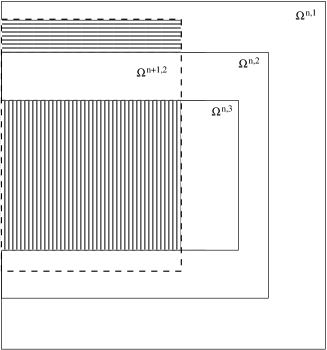
Figure 3: Three grids at time $\tau^{n}$ (solid lines) and a grid at next time step $\tau^{n+1}$ (enclosed by the dashed lines) with the same level as $\mathcal{H}^{n,2}$. In the vertically striped region the new grid coincides with a finer grid at the previous time step, in the horizontally striped region only a coarser grid existed at $\tau^{n}$, and in the region that is not filled a grid at the same level existed at $\tau^{n}$.

4.3.3 Grid mapping

The refinement monitor gives a new grid distribution $\{\mathcal{H}^{n+1,k}\}$ at time $\tau^{n+1}$. In the following we consider mapping functions used to map the solution at $\tau^{n+1}$ on the previous grid distribution $\{\mathcal{H}^{n,k}\}$ on the new grid distribution $\{\mathcal{H}^{n+1,k}\}$. There are three possible relations between a grid $\mathcal{H}^{n+1,k}$ at time $\tau^{n+1}$ and the older grids $\{\mathcal{H}^{n,k}\}$, as illustrated in Fig. 3.

First it is possible that a fine grid $\mathcal{H}^{n,k}$ at the previous time step now is covered by a coarser grid $\mathcal{H}^{n+1,K}$ (as in the vertically striped region of Fig. 3). Then the values of the densities on the new grid are computed by the restriction (4.1):

$$U^{n+1,K}=Res(U^{n,k})\quad\text{ on }\mathcal{H}^{n+1,K}\cap\mathcal{H}^{n,k}\,,$$ (4.4)

where $U$ again stands for the set of grid values of either electron- or ion densities.

Secondly, there is the possibility that (part of) the new grid already existed at previous time step, in which case there is no need for projecting the density distributions from one grid to the other.

Finally, it may occur that the new grid lies on a region where only a coarser grid $\mathcal{H}^{n,K}$ existed at the previous time level (as in the horizontally striped region in Fig. 3). Then we have to prolongate the coarse grid values $U^{n+1,K}$ to the new fine grid. One main consideration in the choice of the prolongation is the conservation of charge in the discretizations. For simplicity, we will first consider a one-dimensional prolongation, which is then easily extended to more dimensions. We consider coarse grid values $U^{K}=\{u^{K}_{I}\}$. Then a mass conserving interpolation for values $U^{k}=\{u^{k}_{i}\}$ on a grid twice as fine is,

$$u^{k}_{i}=U^{K}_{I}+D_{I}\,,\quad u^{k}_{i+1}=U^{K}_{I}-D_{I}\,,$$ (4.5)

which obviously implies mass conservation, $\Delta z^{l}u^{k}_{i}+\Delta z^{l}u^{k}_{i+1}=\Delta z^{L}U^{K}_{I}$. Using a three-points stencil, the coefficient $D_{I}$, such that the interpolation is second order accurate, can be written as

$$D_{I}=\frac{1}{8}(U_{I-1}+U_{I+1})\,.$$ (4.6)

In the case of a three-dimensional geometry with axial symmetry, the above interpolation is applied on $U^{K}$ in the $z$-direction, and on $RU^{K}$ in the radial direction, which ensures mass conservation on such a system.
Remark: This mass conserving interpolation might lead to new extrema or negative values. That could be prevented automatically by limiting the size of the slopes. However, in our simulations this turned out not to be necessary.

Finally, we need boundary values for all grids. On the coarsest grid these simply follow from the discretization of the boundary conditions (2.11)-(2.14), as explained in Sect. 3.1. On finer grids they are interpolated bi-quadratically from coarse grid values. The interpolation error is then third order, and therefore smaller than the discretization error, which would not be the case with a bi-linear interpolation. The quadratic interpolation is derived using the Lagrange interpolation formula to find $U^{k}=\{u^{k}_{ij}\}$ from the coarse grid values $U^{K}=\{u^{K}_{IJ}\}$. The interpolated value becomes

$$u^{k}_{ij}=Int(U^{K})_{ij}=\displaystyle\frac{1}{r^{l(k)}}\sum_{p=-1}^{1}\sum_{q=-1}^{1}r^{l(K)}_{I+p}u^{K}_{I+p,J+q}\prod_{\begin{subarray}{c}P\neq p\\ P=-1\end{subarray}}^{1}\frac{r^{l(k)}_{i}-r^{l(K)}_{I+P}}{r^{l(K)}_{I+p}-r^{l(K)}_{I+P}}\prod_{\begin{subarray}{c}Q\neq q\\ Q=-1\end{subarray}}^{1}\frac{z^{l(k)}_{j}-z^{l(K)}_{J+Q}}{z^{l(K)}_{J+q}-z^{l(K)}_{J+Q}}\,,$$ (4.7)

in which $I=(i+i\mod 2)/2$ and $J=(j+j\mod 2)/2$. We notice that the interpolated quantity again is not $\sigma$ but $r\sigma$ because of the cylindrical coordinate system.

In our algorithm, mass conservation at the grid interfaces will simply be ensured by matching the fluxes of the fine and coarse grids.

4.3.4 Flux conservation at grid interfaces

The mapping from one grid to the other must take into account a flux correction on grid interfaces, in order to ensure mass conservation. This correction yields that the total mass going through one coarse grid cell must be the same as the sum of total mass going through two fine grid cells. Taking into account the cylindrical geometry of the system, the fluxes through coarse grid cells become, in terms of the fine grid fluxes,

$$\begin{array}[]{rcl}F^{K}_{r;I+1/2,J}&=&\displaystyle\frac{\Delta r^{l}}{\Delta r^{L}}(F^{k}_{r;i+1/2,j}+F^{k}_{r;i+1/2,j+1})\,,\\ \displaystyle F^{K}_{z;I,J+1/2}&=&\displaystyle\frac{\Delta r^{l}}{\Delta r^{L}r_{I}}(r^{l}_{i}F^{k}_{z;i,j+1/2}+r^{l}_{i+1}F^{k}_{z;i+1,j+1/2})\,,\end{array}$$ (4.10)

where $i=2I-1$ and $j=2J-1$.

4.4 Refinement scheme for the Poisson equation

The refinement strategy for the computation of the electric potential is also based on a static regridding approach, where the grids are adapted after each complete time step. In this case however, the refinement criterion is not based on a curvature monitor but on an iterative error estimate approach. The Fishpak routine will be used on a sequence of nested grids ${\mathcal{G}}^{m}$. The solution on a coarse grid will be used to provide boundary conditions for the grid on the finer level, which will in general extend over a smaller region. This approach is explained in full detail in [39]; here we will discuss the main features of the scheme.

Starting from the (known) charge density distribution $\sigma-\rho$ on a set of grids $\{\mathcal{H}^{k}\}$, the Poisson equation is first solved on the two coarsest grids ${\mathcal{G}}^{1}$ and ${\mathcal{G}}^{2}$, both covering the entire computational domain $(0,L_{r})\times(0,L_{z})$. The finest of these two grids is coarser or as coarse as the coarsest grid of $\{\mathcal{H}^{k}\}$. The densities should then first be mapped onto the coarse grids ${\mathcal{G}}^{1}$ and ${\mathcal{G}}^{2}$, using the restriction formula (4.1). The source term of the Poisson equation is then known on these two coarse grids, and the Poisson equation is solved using a Fishpak routine that discretizes Eq. (3.3) using second-order differences:

$$\sigma^{m}_{i,j}-\rho^{m}_{i,j}=\frac{\phi^{m}_{i+1,j}-2\phi^{m}_{i,j}+\phi^{m}_{i-1,j}}{(\Delta r^{l})^{2}}+\frac{\phi^{m}_{i+1,j}-\phi^{m}_{i-1,j}}{2r^{l}_{i}\Delta r^{l}}+\frac{\phi^{m}_{i,j+1}-\phi^{m}_{i,j}+\phi^{m}_{i,j-1}}{(\Delta z^{l})^{2}}$$ (4.11)

in which $l=l(m)$ is the level of grid ${\mathcal{G}}^{m}$. This system of linear equations is then solved using a cyclic reduction algorithm, see [40]. The details of Fishpak are described in [37]. The subroutine was used as a black box in our simulations. A comparison with iterative solvers, multigrid or conjugate gradient type, can be found in [41]. For the special problem we have here – Poisson equation on a rectangle – such iterative solvers are not only much slower than Fishpak, but they also require much more computational memory.

As a next step, the coarse grid electric potentials $\phi^{1}$ on ${\mathcal{G}}^{1}$ and $\phi^{2}$ on ${\mathcal{G}}^{2}$ are compared with each other, by mapping $\phi^{1}$ onto ${\mathcal{G}}^{2}$ with a quadratic interpolation based on a nine-point stencil as shown in Fig. 4.

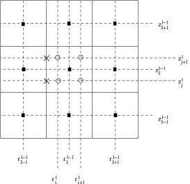
Figure 4: The nine-points stencil used to map coarse grid values of the electric potential $\phi^{l-1}_{IJ}$ onto the fine grid, thus obtaining $\phi^{l}_{i,j}$, $\phi^{l}_{i+1,j}$, $\phi^{l}_{i,j+1}$ and $\phi^{l}_{i+1,j+1}$. The cell centers of the coarse grid are marked with $\scriptscriptstyle\blacksquare$, those of the fine grids with $\circ$, and the boundary points of the fine grids are marked with $\times$.

For the prolongation that gives a continuous map of an electric potential $\phi^{M}=\{\phi^{M}_{IJ}\}$ onto a finer grid ${\mathcal{G}}^{m}$ the following formula, based on a least square fit, is used:

$$\begin{array}[]{lcl}\phi^{m}(r,z)&=&Pro(\;\phi^{M}\,(r,z))\\[5.69054pt] &=&\phi^{M}_{IJ}+c_{10}(r-r^{M}_{I})+c_{01}(z-z^{M}_{J})+c_{11}(r-r^{M}_{I})(z-z^{M}_{J})+\\[5.69054pt] &+&\displaystyle c_{20}(r-r^{M}_{I})^{2}+c_{02}(z-z^{l-1}_{J})^{2}\,.\end{array}$$ (4.15)

For the values of the coefficients $c_{ij}$ we refer to [39]. This interpolation will primarily be used to generate boundary conditions for the finer level, as illustrated in Fig. 4 for the boundary points on the finer grid marked with $\times$, but it will also be used for error estimation. The interpolation for the boundary conditions will be done such that there is a bias in the stencil toward the smooth region to enhance the accuracy.

The error of the solution on a grid $\mathcal{G}^{m}$ is then estimated by the point-wise difference between the solution on that grid and the interpolation of the solution on the underlying coarser grid $\mathcal{G}^{M}$:

$$\tilde{g}^{m}_{i,j}=\phi^{m}_{i,j}-(Pro\;\phi^{M})_{i,j}\,.$$ (4.16)

The refinement criterion is as follows:

$$\text{refine all grid cells $i,j$ where}\;\;|\tilde{g}^{m}_{i,j}|\geq\epsilon_{\phi}$$ (4.17)

where $\epsilon_{\phi}$ is a small parameter that still has to be chosen. This leads to new and finer grids on which the whole procedure of mapping the charge densities onto it, solving the Poisson equation using the Fishpak routine and estimating the error is repeated, and so on either until the error is smaller than $\epsilon_{\phi}$ everywhere or until the finest desired level is reached. Notice that, since the grids do not cover the whole computational domain anymore, the boundary conditions (2.11) do no longer hold. We now have Dirichlet boundary conditions on each boundary that lies in the interior of the computational domain, and they are computed by interpolating the electric potential on the finest grid that is known using Eq. (4.15). Using this third order interpolation formula implies that the error introduced by the interpolation is negligible compared to to discretization error, which is second order. With this method there is an upper bound for the maximum error $e^{m}$ on grid $m$ with level $l$ [39]:

$$e^{m}\leq 3\max_{i,j}\tilde{g}^{m}_{ij}+(l-1)\epsilon_{\phi},$$ (4.18)

where $\tilde{g}^{m}=\max\tilde{g}_{ij}^{m}$ as defined in Eq. (4.16). This means that the extra error due to the refinement can be made as small as wanted provided $\epsilon_{\phi}$ is taken small enough. Therefore, iteration, e.g. with defect corrections, is not needed. Inequality (4.18) is based on the assumption that the interpolation errors are negligible compared to the second-order discretization errors of the local problems, and therefore interpolant (4.15) was chosen to be of higher order. Although tacit smoothness assumptions are involved here, tests in [39] with strong local source terms did show that the errors are indeed well controlled by this nested procedure.

We notice that this global error control is the reason for the choice of this particular refinement monitor for the Poisson equation. Such an error control does not hold for the continuity equations, for which we use the more suitable curvature monitor [34, 38].

The electric field has to be known on the continuity grids ${\mathcal{H}^{k}}$, since it appears in the continuity equations (2.8)-(2.9). However it has to be computed from the electric potential that is only known on the Poisson grids, using Eq. (3.4). We consider the grid $\mathcal{H}^{k}$ with level $l(k)$ on which the electric field has to be known, and the finest potential grid $\mathcal{G}^{m}$ with level $l(m)$, which has a non-empty intersection with $\mathcal{H}^{k}$.

There are three possible situations: the potential grid can be either coarser, as fine as, or finer than the continuity grid. If both grids have the same size ($l(k)=l(m)$), or if the continuity grid is coarser than the Poisson grid ($l(k)<l(m)$), then the field components are set directly with a second order central approximation of Eq. (3.4), using the neighboring points of the point where the field components need to be known. If the Poisson grid is coarser than the continuity grid ($l(k)>l(m)$), the electric field is first computed on the Poisson grid with a second order central approximation of Eq. (3.4), and then this field is interpolated to the continuity grid. The interpolation is performed with a piecewise bilinear approximation.

4.5 Overall algorithm

In previous sections, the refinement algorithms for the continuity equations and the Poisson equation have been treated separately. We here describe the overall algorithm.

We start from known density distributions of the charged particles $\sigma^{n}$ and $\rho^{n}$ at a certain time $\tau^{n}$, on a set of grids ${\mathcal{H}^{n,k}}$. The electric field induced by the charges on the grids ${\mathcal{H}^{n,k}}$ is computed using the refinement method described in Sect. 4.4.

The step size for the time integration is then set in such a way that the stability conditions (3.30)-(3.31) of both advection and diffusion discretizations are met on the finest grid. The values of both $\nu_{a}$ and $\nu_{d}$ have been taken as 0.1. This is smaller than the maximal values of 0.87 and 0.37 specific to the third-order upwind scheme for the advection and the second-order central discretization for diffusion, respectively, together with a two-stage Runge Kutta time integration method [32].

Then, starting on the finest grid level, the particle fluxes are computed on each grid and corrected using the flux correction formulas (4.10). Then the first stage of the Runge Kutta step (3.26) is carried out. The field induced by the density predictors $\bar{\sigma}^{n}$ and $\bar{\rho}^{n}$ is again computed using the procedure described in Sect. 4.4. The new boundary conditions for the particle densities are computed on all grids ${\mathcal{H}^{n,k}}$, and the second stage of the Runga-Kutta method is carried out in the same way as the first stage. We then obtain the density distributions $\sigma^{n+1}$ and $\rho^{n+1}$ on the set of grids ${\mathcal{H}^{n,k}}$.

Following the procedure described in Sect. 4.3, after restriction of fine grid values to the parent grids, the grids ${\mathcal{H}^{n+1,k}}$ for the next time step are computed using the refinement monitor (4.3). The densities are then mapped from the grids ${\mathcal{H}^{n,k}}$ to the grids ${\mathcal{H}^{n+1,k}}$, and the new boundary conditions are computed. We thus obtain the density distributions $\sigma^{n+1}$ and $\rho^{n+1}$ on the set of grids ${\mathcal{H}^{n+1,k}}$ at the new time $\tau^{n+1}$.

4.6 Relations with other refinement algorithms

As mentioned before, the initial attempts to solve the system (3.1)-(3.4) were done by using the existing adaptive finite difference code VLUGR [34]. This code failed for our problem. Another unsuccessful attempt was made using the adaptive finite element code KARDOS [42]. Both these codes use implicit time stepping, and they do not take into account the unstable behavior of the solution ahead of the front.

Since our algorithm uses explicit (Runge-Kutta) time stepping, the refinement procedure is relatively simple. In particular, the computation for the electric potential becomes decoupled from the density updates in the continuity equations. This allows for a tailored approach to these separate problems. The potential updates are performed using nested fast Poisson solvers [39], which requires rectangular (nested) regions for these sub-problems together with a high-order interpolant for a global error indicator. For the continuity equations, on the other hand, the computational regions can be chosen quite small, essentially confined to the streamer itself. For these equation the simple error monitor based on local curvature performs well.

Local time stepping, for the different grids on parts of the domain, have not been considered in this paper. Although savings might be expected for the continuity equations, where we now use the same time step dictated by the finest mesh, such approach would lead to the complication that also the potential needs to be updated locally, and that charge conservation is no longer straightforward.

A grid refinement approach with fixed, a priori chosen, grids but with local time stepping has been discussed in [43] for a, somewhat related, system of plasma equations. The main difference with our problem is that this system is considered with low electric fields but on a much larger time scale, with movement of ions described by Euler equations. The time step restriction (3.33) for dielectric relaxation then becomes very severe. To overcome this restriction, an implicit treatment of the potential in the electron drift fluxes is required. In the approach of [44, 43] this is done through (3.20) together with a low-order prediction update for the electron densities. The other processes, including higher-order corrections, are solved in a time-split fashion. With local time steps, synchronization at the new (global) time level is needed to ensure the relevant conservation properties to hold, such as charge conservation. Apparently, the instabilities in the leading edge are not that much of a problem on the time scales considered in these papers, probably because the charged fronts are smoother.

Some results based on non-uniform, moving grids have been reported [24], for the simulations of streamers originating from point electrodes. The regridding approach used in [24] allows only for a fixed number of grid points, and does not seem to take into account properly the leading edge. In contrast, the method presented in this article enables a a fine grid to be put wherever needed, in particular, over the leading edge.

We are not aware of other grid refinement approaches for systems of plasma equations that do take this leading edge instability into account. Related problems have been reported however in [45] with moving mesh methods for the 1D Fisher equation $u_{t}=u_{xx}+\gamma u(1-u)$. To overcome instability of the numerical moving mesh scheme, a special monitor function was advised in [46]. This has essentially the effect of mesh refinement ahead of the front. It seems that extensions of this moving mesh approach to multidimensional reaction-diffusion equations or more complicated systems have not been implemented yet.

5 Tests of the algorithm on a planar ionization front

The implementation of the grid refinements is first tested on the evolution of a planar streamer front. As analytical results for this case are available [12], any errors in the implementation can be identified. Moreover, conclusions on the tolerances and interpolations can be drawn for the more general two-dimensional simulations.

A one-dimensional simulation is carried out with the two-dimensional code by letting initial and boundary conditions depend on $z$ only and not on the radial coordinate $r$. Specifically, the initial ionization seed

$$\sigma(r,z,0)\;=\;\rho(r,z,0)\;=\;10^{-2}\;e^{-(z-z_{b})^{2}}$$ (5.1)

is located at $z=z_{b}$ and a constant background electric field ${{\boldsymbol{\mathcal{E}}}_{b}}=-|{\boldsymbol{\mathcal{E}}}_{b}|{\bf\hat{e}_{z}}$ is applied. The spatial region in this specific example is $(r,z)\in[0,L]\times[0,L]$ with $L=1024$. The boundary conditions for the electron density and the electric potential in this specific case are

$$\begin{array}[]{l}\displaystyle\sigma(r,0,\tau)=0\,,\quad\frac{\partial\sigma}{\partial z}(r,L,\tau)=0\,,\quad\frac{\partial\sigma}{\partial r}(0,z,\tau)=0\,,\quad\frac{\partial\sigma}{\partial r}(L,z,\tau)=0\,,\\[11.38109pt] \displaystyle\phi(r,0,\tau)=0\,,\quad\frac{\partial\phi}{\partial z}(r,L,\tau)=|{\boldsymbol{\mathcal{E}}}_{b}|\,,\quad\frac{\partial\phi}{\partial r}(0,z,\tau)=0\,,\quad\frac{\partial\phi}{\partial r}(L,z,\tau)=0\,.\end{array}$$ (5.2)

In this situation, the electric field does not depend on $r$. It can be written as ${\boldsymbol{\mathcal{E}}}(r,z,\tau)={\mathcal{E}}(z,\tau){\bf\hat{e}_{z}}$, and it can be obtained directly from the charge densities by integrating $\nabla\cdot{\boldsymbol{\mathcal{E}}}=\rho-\sigma$ from Eq. (2.10) along the $z$-direction and using the boundary condition ${\mathcal{E}}=-|{\boldsymbol{\mathcal{E}}}_{b}|$ for the electric field at $z=L$. The result is

$${{\mathcal{E}}}(z,\tau)=-|{\boldsymbol{\mathcal{E}}}_{b}|+\int_{z}^{L}\left(\sigma(z^{\prime},\tau)-\rho(z^{\prime},\tau)\right)\>dz^{\prime}.$$ (5.3)

This means that it is not necessary to calculate the electric potential $\phi$. Rather the electron and positive ion density at time $t^{n}$ determine the electric field ${\mathcal{E}}^{n}$ at each cell vertex by discretizing Eq. (5.3). Starting from the value at $z=L$, which corresponds to $j=M$ on a grid with $M$ grid points in the $z$-direction, we thus obtain:

$${{\mathcal{E}}}^{n}_{M+\frac{1}{2}}=-|{\boldsymbol{\mathcal{E}}}_{b}|\,,\qquad{{\mathcal{E}}}^{n}_{j-\frac{1}{2}}={{\mathcal{E}}}^{n}_{j+\frac{1}{2}}+\Delta z(\sigma^{n}_{j}-\rho^{n}_{j})\;\;{\rm for}~{}j\leq M\,.$$ (5.4)

The electric field strength in the cell centers is then taken as the average field of the corresponding vertices,

$$|{\mathcal{E}}|^{n}_{j}=\frac{1}{2}\left|{\mathcal{E}}^{n}_{j-\frac{1}{2}}+{\mathcal{E}}^{n}_{j+\frac{1}{2}}\right|$$ (5.5)

We emphasize that in this section, in which the particular case of a one-dimensional streamer front is considered, we use Eqs. (5.4)-(5.5) to compute the electric field, rather than the Poisson equation. This speeds up considerably the computations, and enables us to test the refinements for the continuity equations only. For tests on the refinements of the Poisson equation only we refer to [39].

Fig. 5 shows the temporal evolution of the initial ionization seed (5.1) located at $z_{b}=31$, with a background field $|{\boldsymbol{\mathcal{E}}}_{b}|=1$ and a diffusion coefficient $D=0.1$. The results shown are obtained on a uniform grid with mesh spacings $\Delta r=32$ and $\Delta z=1/4$, which will be considered afterwards as a reference solution. $z_{b}$ is chosen large enough that boundary effects at $z=0$ do not matter. and that the initial maximum is well presented even in the case treated later in which a coarse grid with mesh size $\Delta z=2$ is used. After an initial growth until time $\tau\approx 25$, an ionization front emerges that moves with about constant velocity to the right in the direction opposite to the background field.

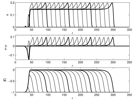
Figure 5: Numerical solutions of the planar streamer front with $|{\boldsymbol{\mathcal{E}}}_{b}|=1$ and $D=0.1$ for $0\leq\tau\leq 200$ with time steps of 10. The solution is computed on a uniform grid with a mesh spacing of $1/4$ in the direction of propagation. The thick lines correspond to multiples of 50 for $\tau$.

The front velocity as a function of time is plotted in Fig. 6. It is derived from the numerical displacement of the level $\sigma_{f}=10^{-8}$ within a time interval of 10. The front decelerates and eventually approaches a value somewhat below the asymptotic front velocity [12]

$$v^{\ast}=|{\boldsymbol{\mathcal{E}}}_{b}|+2\sqrt{D|{\boldsymbol{\mathcal{E}}}_{b}|e^{-1/|{\boldsymbol{\mathcal{E}}}_{b}|}}$$ (5.6)

which for these particular values of the background electric field and the diffusion coefficient is equal to 1.3836. The numerical velocity at large times is around 1.365 which corresponds within an error margin of 1.5% to the asymtpotic value. We expect to obtain even better results on finer grids, but we focus in what follows on the performance of the refinement algorithm compared to this uniform grid computation. For further discussion of the results we refer to Appendix B. Moreover, deviations from this asymptotic value can be derived analytically for different numerical schemes, and that this is illustrated in Section 5.6.6 of [25] for an explicit and a semi-implicit time discretization of a diffusion equation.

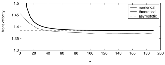
Figure 6: Numerical front velocity (thin solid line) as a function of time, compared to the theoretical front velocity (thick line, derived in Appendix B) and the theoretical asymptotic front velocity $v^{\ast}=1.3863$

In the following illustrations we have computed the temporal evolution of the densities and the electric field on a fine ($\Delta z=1/4$) and on a coarse ($\Delta z=2$) uniform grid as well as on locally refined grids. In the latter case, the coarsest grid has a mesh spacing of $\Delta z^{c}=2$ which we refine up to a finest mesh width of $\Delta z^{f}=1/4$, thereby allowing for three levels of refinement. The electric field is again computed using Eq. 5.4 rather than through the Poisson equation for the electric potential, which speeds up the computations. The refinement algorithm for the continuity equations is as explained in Sect. 4.3. To demonstrate that the leading edge has to be included in the refinement, results with the “standard” refinement (i.e. without including the leading edge) will be compared to those that do include the leading edge. In this leading edge of the ionization front the densities decay exponentially, but the electric field strength is such that the reaction term is non-negligible. From theoretical studies [12] as briefly recalled in Appendix B it is known that this region is very important since it determines the asymptotic dynamics of the front.

For the present problem we use the a priori knowledge that the front moves to the right and the leading edge is the region ahead of the front. The standard criterion reads,

$$\text{refine all grid cells $j$ where}\;\;\Big{|}\frac{\partial^{2}u}{\partial z^{2}}(z_{j})\Big{|}\geq\epsilon_{u},\quad u=\sigma,\,\sigma-\rho$$ (5.7)

Second, we use the same criterion but now with the inclusion of the so-called leading edge in the refined region, taking into account the cut-off of densities below the continuum threshold of 10^-12, i.e.:

$$\begin{array}[]{l}\text{refine all grid cells $j$ obeying criterion (\ref{refcrit1})},\\ \text{extend the refined region in the propagation direction}\\ \text{to all $\{z_{j}|\sigma_{j}>10^{-12}\}$.}\end{array}$$ (5.8)

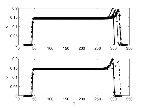
Figure 7: Performance of the refinements without and with inclusion of the leading edge. Plotted is $\sigma(z,\tau)$ as a function of $z$ for $\tau=200$. Upper row: results on grids refined with the standard criterion with a tolerance of $10^{-3}$ (circles) and $10^{-8}$ (pluses) compared to a fine grid computation ($\Delta z=\frac{1}{4}$, thick solid line) and a coarse grid computation ($\Delta z=2$, thick dash dotted line). Lower row: the same, but now with leading edge included in the refinement, only shown with a tolerance of $10^{-3}$.

The upper and lower plot of Fig. 7 show the results of the one-dimensional streamer simulation computed with the criterion 5.7 and 5.8, respectively, together with a coarse and a fine uniform grid computation. The time step is such that the Courant numbers for both advection and diffusion are at most 0.1, which is sufficiently small to render the temporal errors negligible.

The value of $z_{b}$ in the initial pulse (5.1) has been chosen such that the maximum of this Gaussian pulse was situated in a coarse grid cell center. Moreover, if a grid refinement is needed at the very first time step, the initial condition on the finer grids is not interpolated from the coarser grid values, but is calculated directly from Eq. (5.1), so that the initial pulse on the finer grids is computed without interpolation errors.

The results with a fine uniform grid can be considered as a reference solution, and it is clear that on the coarse uniform grid the front moves too fast and is too smooth. This is due to the large amount of numerical diffusion introduced by the coarse grid. As can be concluded directly from the expression for the asymptotic front velocity, a larger diffusion constant leads to a larger velocity, and a larger velocity makes the front smoother [12].

The same is observed on the grids refined according to the standard criterion, even with a very strict tolerance the front is badly captured. This also appeared with other standard refinements codes, e.g. VLUGR [34] The major conclusion from this failure is that the refinement takes place at the wrong place, namely at the regions with steep gradients. This is not where the dynamics of a pulled front is determined. This occurs rather in the leading edge where any perturbation of the linearly unstable state will grow [12]. Therefore the method in which the leading edge is included in the refined region gives even with a relatively low tolerance much better results than the standard refinement strategy.

In Table 1 the front velocities $v_{f}$ are listed for the fine ($\Delta z=\frac{1}{4}$) and the coarse ($\Delta z=2$) uniform grids, as well as for refined grids ($\Delta z^{c}=2$, $\Delta z^{f}=\frac{1}{4}$) with or without inclusion of the leading edge, and with linear or quadratic interpolation of the boundary conditions; the tolerance is set to $\epsilon_{\sigma}=\epsilon_{\sigma-\rho}=10^{-3}$. The velocities in the table have all been determined from the displacement of the maximal electron density between $\tau$=250 and 262.5. As explained before [12], the numerically computed front velocities should be smaller than the theoretical value, which is indeed the case for the fine grids.

We also looked at the results obtained by discretizing the advective term with a first-order upwind scheme. We concluded from those tests that this scheme performs very badly, quite in contrast to what is said in [24]. The amount of numerical diffusion introduced by that scheme completely changes the asymptotic velocities on realistic grids. Moreover, numerical diffusion can be expected to over-stabilize the numerical scheme [32] and to suppress thereby interesting features of the solutions such as streamer branching.

Table 1: Front velocities $v_{f}$ on various grids. The refinements have been carried out with $\epsilon_{\sigma}=\epsilon_{\sigma-\rho}=10^{-3}$. The exact asymptotic velocity is $v^{\ast}=1.3836$. For comparison, results for the 1st-order upwind scheme on the fine grid are added.

method	$v_{f}$
uniform $\Delta z=\frac{1}{4}$, 1st-order upw.	1.585
uniform $\Delta z=\frac{1}{4}$, flux limited	1.365
uniform $\Delta z=2$, flux limited	1.448
standard refinement	1.469
refinement including leading edge	1.365

From these tests it appears that the grid refinement based on a simple curvature monitor works well provided the leading edge is included in the regions of refinement. This is in accordance with [12] where the importance of the leading edge for dynamics of a planar front is discussed.

6 Performance of the code on streamer propagation with axial symmetry

A planar ionization front as treated in the previous section is mainly of theoretical interest. Genuine ionization fronts are curved around the streamer head, which leads to field enhancement ahead of the front. We now consider the streamer propagation with cylindrical symmetry (2D case), which differs substantially from the planar front (1D case), mainly due to the field enhancement ahead of a curved front. In particular, the electric field cannot be calculated as easily as in Eq. (5.3), but has to be computed through the Poisson equation for the electric potential. The tolerance $\epsilon_{\sigma-\rho}$ will play a non-negligible role in that case. Also, as the electric field is enhanced immediately ahead of the ionization front and decreases further ahead, the leading edge region of maximal linear instability of the non-ionized state is bounded.

In this section the refinement algorithm as presented in Sect. 4 will be applied to a streamer initiated by a Gaussian ionization seed situated on the axis of symmetry at the cathode, $z=0$.

$$\sigma(r,z,0)=\rho(r,z,0)=10^{-4}\exp\left(-\frac{r^{2}+z^{2}}{100}\right)\,.$$ (6.1)

The computational domain is $L_{r}$=1024 and $L_{z}$=2048, and the background electric field is set to $|{\boldsymbol{\mathcal{E}}}_{b}|=0.5$. We use homogeneous Neumann boundary conditions at the cathode ($z=0$), which, together with the ionization seed placed on the cathode, means that electrons flow into the system. For other boundary conditions we refer to Sect. 2.3.

The temporal evolution of the ionization seed (6.1) under these conditions is shown in Fig. 8.

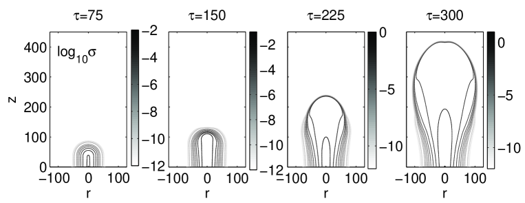
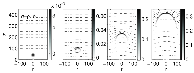
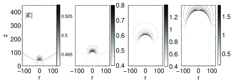
Figure 8: Propagation of a Gaussian ionization seed as given by Eq.(6.1) in a background field $|{\boldsymbol{\mathcal{E}}}_{b}|=0.5$. The snapshots correspond to times $\tau$=75, 150, 225 and 300. The upper row gives the logarithm of the electron density $\sigma$, the middle row the net charge density $\sigma-\rho$ and the lower figure the electric field strength $|{\boldsymbol{\mathcal{E}}}|$. A uniform grid $\Delta r=\Delta z=1$ has been used for both the continuity equations and the Poisson equation.

A uniform grid with grid size $\Delta r=\Delta z=1$ covers the domain where both the electron and positive ion densities are strictly positive. This is a relatively coarse grid, but, as mentioned in Sect. 4.1, the use of finer grids would require too many grid points for the Fishpak routine to handle within an acceptable accuracy. Therefore we will use this uniform grid computation as a reference to test the performance of the adaptive refinement method. Fig. 8 shows the snapshots of the electron and net charge density distributions as well as the electric field, at $\tau=75$, 150, 225 and 300.

At $\tau=75$, the maximal deviation of the electric field strength from its background value is around 0.4%, and space charges do not play a significant role yet. This is the electron avalanche phase, during which the Gaussian electron density distribution advects with an almost constant velocity, undergoes a diffusive widening, and grows due to impact ionization, leaving behind a small trail with positive ions [47].

At $\tau=150$ the space charges concentrate in a layer around the streamer head, as can be seen in the second column of Fig. 8. Due to its curvature, this space charge layer focuses the electric field towards the axis of symmetry, thereby enhancing it. The body of the streamer is sufficiently ionized (and its conductivity therefore enhanced) and the electric field in the streamer body is lower than the background field. The space charge layer becomes thinner and denser in time, and the electric field is increasingly enhanced, as can be seen in the third column of Fig. 8.

Eventually, the streamer becomes unstable, and branches. The beginning of this branching state is shown in the rightmost column of Fig. 8.

Let us now consider the effect of the refinements on the streamer dynamics, as well as the effect of cutting off the densities that are below the continuum threshold. To this end, we run the simulations with the same parameters – background field, initial and boundary conditions – as in the previous subsection, but we now allow one level of refinement for the continuity equations, and seven levels of refinement for the Poisson equation. The finest grids in both cases have a finest mesh size $\Delta r^{f}=\Delta z^{f}=1$. In the next section, more levels of refinement will be used. In Sect. 5 we could see that, provided the leading edge of the streamer front is included in the refinement, and a quadratic interpolation is used to provide the boundary conditions for finer grids, a tolerance for the continuity equations of $\epsilon_{\sigma}=10^{-3}$ is well suited. Moreover, the error in the spatial discretization of the net charge density $\sigma-\rho$ is induced by the discretization of the drift and diffusion terms in Eq.(2.8). Hence it is natural to take the tolerance for the net charge density equal to that for the electron density.

The choice for the tolerance for the refinement of the Poisson equation is less straightforward. In one dimension, the error in the second order discretization of the Poisson equation (2.10) reads

$$\delta\phi=\frac{\Delta z^{2}}{12}\frac{\partial^{4}\phi}{\partial z^{4}}=\frac{\Delta z^{2}}{12}\frac{\partial^{2}(\sigma-\rho)}{\partial z^{2}}\,.$$ (6.2)

Therefore, in the one-dimensional case, the curvature monitor for the net charge density will also give the error in the spatial discretization of $\phi$. In higher dimensions however, this correspondence does not strictly hold anymore. Nevertheless we assume that the tolerance for $\sigma-\rho$ will still give a good estimation for the error in the solution of the Poisson equation, and we therefore take

$$\epsilon_{\phi}=\epsilon_{\sigma-\rho}=\epsilon_{\sigma}=10^{-3}\,.$$ (6.3)

The number of grid points in the $r-$direction contained in each fine grid for the continuity equations has be chosen as $M_{0}=32$.

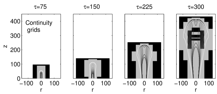
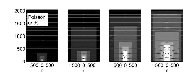
Figure 9: Grid distributions for the continuity equations (upper row), and for the Poisson equation (lower row). The times are the same as in Fig. 8. For the continuity grids, the black regions correspond to the coarsest grid with $\Delta r^{c}=\Delta z^{c}=2$, and which covers the domain on which the particle densities are above the continuum threshold. The gray regions are covered with the fine grids with $\Delta r=\Delta z=1$. The two coarsest grids – with $\Delta r=\Delta z=128$ and 64 – on which the Poisson equation has been solved cover the whole computational domain, which is filled in black. The finer grids with cell size 32, 16, 8, 4 and 2 are plotted in lighter gray shades, the white grid corresponds to $\Delta r^{f}=\Delta z^{f}=1$.

The net charge density distribution at $\tau=75$, 150, 225 and 300 are plotted in the upper row of Fig. 9, together with the grids on which the continuity equations have been solved. The equipotential lines are shown together with the grid distribution for the Poisson equation in the lower panel of Fig. 9.

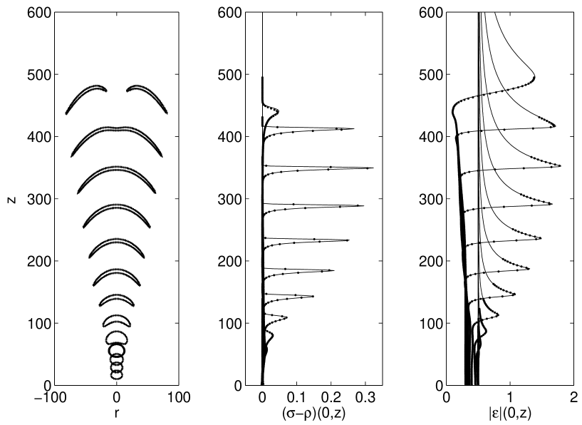
Figure 10: Comparison of uniform grid results with those obtained using the grid refinement strategy. Left panel: evolution of the half maximum contours of the net charge density. Middle panel: evolution of the net charge density on the axis of symmetry, $(\sigma-\rho)(0,z,\tau)$. Right panel: evolution of the electric field strength on the axis of symmetry, $|{\boldsymbol{\mathcal{E}}}|(0,z,\tau)$. The results in all panels are shown for $\tau=25$ to 325, with steps of 25. Solid line: uniform grid ($\Delta r=\Delta z=1$), dots: grid refinement ($\Delta r=\Delta z=1,2$).

Since the streamer front is not planar anymore, it is necessary to investigate the effect of the refinements not only on the axis, but in the whole streamer. The evolution of the half maximum contours of the net charge density is depicted in the left plot of Fig. 10, both in the uniform grid computation without cut-off below the continuum threshold, and with the refinements including the cut-off. There is an excellent correspondence between the uniform grid computation and the one where all grids are refined. At some places there is a slight difference between the results, but this is also a consequence of the results being plotted for the coarsest grid, i.e. $\Delta r^{c}=\Delta z^{c}=1$ for uniform grid, and on $\Delta r^{c}=\Delta z^{c}=2$ for the refined grids. The grid points on which the results are plotted therefore do not coincide, and the contours consequently might be slightly different. Up to branching however, there is no significant error in either the radius or the width of the space charge layer. A minor effect of the refinement only becomes visible once the streamer has become unstable. A more detailed investigation of this branching will follow in a later paper.

The leftmost plot of Fig. 10 has to be completed with the evolution of the axial charge density distribution of the streamer, in order to control not only the position of the half maximum contours, but also the maxima themselves. This is shown in the middle and rightmost plots of Fig. 10, where the axial charge density and electric field strength distributions, respectively, are shown for the same times as the leftmost plot of Fig. 10. Again it appears that the adaptive grid refinement method produces results that coincide very well with the uniform grid computation.

Finally, because of the charge conservation during an ionization event, it should be verified that the refinements are indeed mass conserving, as has been taken care of in Sect. 4.3. This is shown in Fig.11, where we have compared a uniform grid computation where the densities below the continuum threshold have not been cut off, with the refined grid computation. It is clear that neither the cut-off, nor the refinement disturb the total number of particles in a visible way.

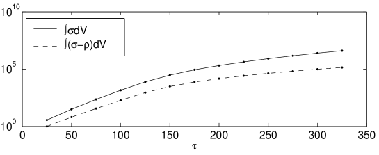
Figure 11: Evolution of the total number of electrons (solid line) and net charge (dashed line). The lines correspond to a uniform grid computation without cutting off the densities below the continuum threshold, the dots to the refined grid computation.

The gain in memory obtained with the refinement method can be observed through the number of grid points that are used to solve the continuity equations and the Poisson equation. As can be seen in Fig.12, the number of grid points used are one to three orders of magnitude smaller than in the computations as performed in [14], where a uniform grid covers the whole computational domain. For the gain in CPU time, we refer to table 2 in the next section.

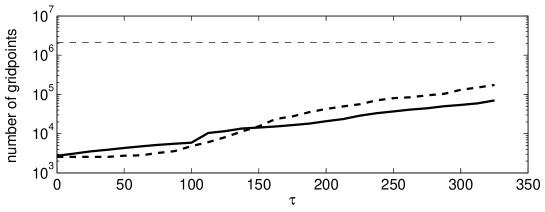
Figure 12: Number of grid points as a function of time. The thin dashed line represents the number of grid points corresponding to a grid of grid size $\Delta r=\Delta z=1$ over the whole domain, i.e. 1024$\times$2048. The thick lines give the temporal evolution of the number of grid points when the refinement algorithm is applied up to a finest mesh size of $\Delta r=\Delta z=1$. Solid line: continuity equations, 1 level of refinement. Dashed line: Poisson equation, 6 levels of refinement.

We emphasize that in the previous test the choice for two levels of refinements has been made in order to compare the results with uniform grid computations. In later simulations we will use more refinement levels, thereby reaching much smaller mesh sizes. We can however extrapolate the outcome of these tests to cases using more levels.

7 Accuracy requirements for the streamer simulations

To illustrate the use of the above algorithm, we present results in a new parameter regime, namely in a very long gap with relatively low background field, and a short gap with high field. We present results on different finest mesh sizes, and investigate the convergence of the solution on decreasing the finest mesh.

7.1 Long streamers in a low electric field

We consider a gas gap on which a background electric field $|{\boldsymbol{\mathcal{E}}}_{b}|=0.15$ is applied. The negative electrode (cathode) is placed at $z=0$, the positive one (the anode) at a distance $L_{z}=2^{16}=$65 536. The radial boundary is situated at $L_{r}=2^{(}15)=$32 768. For N₂ at atmospheric pressure, this corresponds approximately to an inter-electrode distance of 15 cm and an electric field of 30 kV/cm.

The initial seed (2.13) is placed on the cathode at $z=0$ ($z_{b}=0$). The maximal initial density is $\sigma_{0}=1/4.7$ and the e-folding radius of the seed is $R_{b}=10$, which correspond to a density of 14 cm^-3 and a radius of 23 $\mu$m, respectively, for N₂ under normal conditions. This relatively dense seed enables us to bypass the avalanche phase. If we would start with a single electron at this value of the electric field, analytical results [47] show that the transition to streamer would occur after the avalanche has traveled a distance $d\approx 18\alpha^{-1}(|{\boldsymbol{\mathcal{E}}}_{b}|)\approx$ 14 000. Using a dense seed accelerates the transition time considerably. The dense seed mimics streamer emergence from a needle inserted into the cathode or from a laser induced ionization seed.

The coarsest grid for the continuity equations has a mesh size of 64 in both directions, the coarsest one for the Poisson equation a size of 8192. We first present the results when the grids are refined up to a mesh size $\Delta r^{f}=\Delta z^{f}=2$.

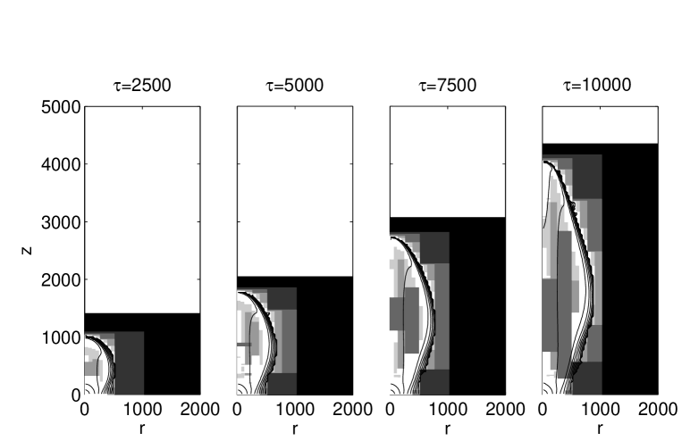
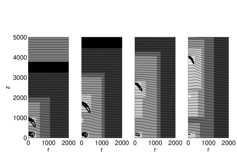
Figure 13: Evolution of a streamer and the computational grids in a low background electric field $|{\boldsymbol{\mathcal{E}}}_{b}|=0.15$. Upper panel: logarithm of the electron density with the grids for the continuity equations. The coarsest grid with mesh size 64, covering the domain on which the continuum approximation for the densities holds, is filled in black. The finest grids with mesh size 2 are white. The particle densities in the white region ahead of the streamer are below the continuum threshold and therefore not solved. Lower panel: net charge density (thick lines) and equipotential lines (thin lines) together with the grids for the Poisson equation. The white domains are covered with the finest mesh size of 2, the black regions are covered by a grid with mesh size 64. The gray region ahead of the streamer at $\tau$=2500 is covered by a grid with mesh size 128. The coarser grids (with mesh sizes up to 8192) are not shown.

The upper panel of Fig. 13 shows the electron density distribution on a logarithmic scale. There are two regions in the streamer: a rather wide one with low electron densities, and one which is much narrower and very dense. The lower panel of Fig. 13 clearly shows the negatively charged layer and its effect on the equipotential lines. These are close to each other ahead of the streamer tip, which indicates an enhancement of the electric field. In the interior field the distance between the equipotential lines is slightly larger than outside the streamer, which implies that the field in the streamer body is somewhat smaller than the background field.

Let us now compare these results with those obtained on coarser grids. We have run the simulations on grids that were refined up to mesh sizes of $\Delta r^{f}=\Delta z^{f}=4$ and $\Delta r^{f}=\Delta z^{f}=8$, thus the finest grids in these cases are twice respectively four times coarser than those on which the results shown in Fig. 13 have been obtained.

Fig. 14 shows the influence of the mesh size by means of the net charge density distribution and the electric field. The leftmost plot of this figure shows the evolution of the half maximum contours of the net charge density. The evolution of the density distribution and the electric field strength are shown in the middle and rightmost plot, respectively. Up to $\tau\approx 5000$ we see that the coarse grid simulations ($\Delta z^{f}=8$) already give convergent results. After this time, the front starts to move somewhat too fast on this coarse grid. This is due to numerical diffusion. The simulation with $\Delta z^{f}=4$ gives the same results as those on a grid with size $\Delta z^{f}=2$ up to $\tau\approx 7500$, after which numerical diffusion again makes the front move somewhat too fast. We emphasize However, the influence of the grid becomes significant only around $\tau\approx 10000$, when the streamer head becomes unstable. The effect of the grid size on the streamer instability will be considered in more detail in a future paper.

We notice that the solution on a grid with mesh spacing 8 eventually lags behind the fine grid computation. This non-monotonous behavior is due to a competition between two opposite effects: the numerical diffusion tends to accelerate the field, but also to reduce the maximum of the charge distribution, thereby reducing the maximal electric field strength, and thus the propagation velocity of the streamer.

In Fig. 15 we compare the evolution of the maximal net charge density on the axis of symmetry for different choices of the finest mesh size. It shows that, the coarser the grid, the more underestimated the maximal net charge density becomes. This indicates that it is indeed numerical diffusion which smears out the space charge layer, thereby accelerating it and decreasing its density.

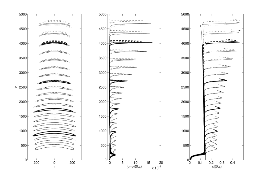
Figure 14: Influence on the mesh size on the numerical solution for a background field of 0.15. The left panel shows the evolution of the half maximum contours of the net charge density $\sigma-\rho$. To show the structure clearly, the aspect ratio is not equal. The middle and the right panels show the evolution of the net charge density and the electric field strength on the axis, respectively. The times shown go from 500 to 11000 with equidistant time steps of 500. The thick lines correspond to the times shown in Fig. 13. Solid line: $\Delta z^{f}$=2; dashed line: $\Delta z^{f}$=4; dotted line: $\Delta z^{f}$=8.

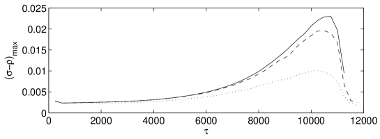
Figure 15: Temporal evolution of the maximal net charge density on the axis. Solid line: $\Delta z^{f}$=2; dashed line: $\Delta z^{f}$=4; dotted line: $\Delta z^{f}$=8.

We conclude that the simulations run on a finest grid with mesh size 8 will give non-negligible errors in the results. However, one more level of refinement, leading to a finest grid with mesh size 4, already gives acceptable solutions during the streamer regime. Moreover, from these results, we can extrapolate that refining the grids even more (e.g. up to a finest mesh size of 1) will not lead to a significant correction of the results, and that the computational work required to run the simulations on such fine grids is not in proportion with the gain in accuracy.

7.2 Fine grid computations at a high electric field

We now consider the evolution of a streamer in a short overvolted gap. The inter-electrode distance is set to 2048, corresponding to 5 mm for N₂ at atmospheric pressure. The background electric field is set to ${\boldsymbol{\mathcal{E}}}_{b}=-0.5{\bf\hat{e}}_{z}$, which corresponds to 100 kV/cm. The initial seed (2.13) is placed on the cathode ($z_{b}=0$). The maximal density of the initial seed is set to $\sigma_{0}=10^{-4}$, and its radius to $R_{b}=10$.

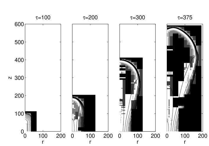
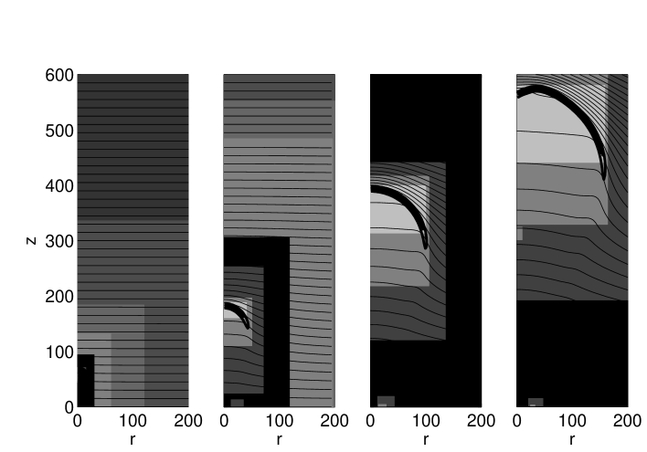
Figure 16: Evolution of a streamer and the computational grids in a high background electric field $|{\boldsymbol{\mathcal{E}}}_{b}|=0.5$. Upper panel: logarithm of the electron density together with the grids for the continuity equations. The coarsest grid has a mesh size $\Delta z^{c}=2$ and is filled in black. The finest grid has a mesh size of $\Delta z^{f}=1/8$ and is white. The white region surrounding the coarsest grid has not been covered by a computational grid since the densities are below the continuum threshold there. Lower panel: net charge density (thick lines) and equipotential lines (thin lines) together with the grids for the Poisson equation. The black region is covered with a grid with mesh size 2, coarser grids are not shown on this scale. The grids are refined up to a mesh of $\Delta z^{f}=1/8$. However, this finest grid is only used at $\tau$=375, in a very small part of the computational domain. The finest grid for the Poisson equation at $\tau$=100 has a mesh size of 1. At $\tau$=200 and 300 the finest grid has a mesh size of 1/4.

The evolution of the streamer with previous initial and boundary conditions, during the non-linear phase is shown in Fig. 16. These results have been obtained on finest grids with a mesh size of $\Delta z^{f}=1/8$ for both the continuity and the Poisson equations. The coarsest grid for the continuity equation has a mesh size of $\Delta z^{c}=2$, the one for the Poisson equation has a size of $\Delta z^{c}=128$.

The discharge clearly exhibits the streamer features which are, as in the low field case, a thin negatively charged layer that enhances the electric field ahead of it, and partially screens the interior of the streamer body from the background electric field.

In order to investigate the convergence of the solution under decreasing grid size, we have also run the simulations on finest mesh sizes $\Delta z^{f}=1/4$, $\Delta z^{f}=1/2$ and $\Delta z^{f}=1$. Fig. 17 shows the evolution of the half maximum contours of the net charge density, as well as that of the axial distribution of the net charge density and the electric field strength.

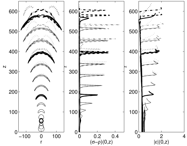
Figure 17: Influence on the mesh size on the numerical solution for a background field of 0.15. The left panel shows the evolution of the half maximum contours of the net charge density $\sigma-\rho$. The middle and the right panels show the evolution of the net charge density and the electric field strength on the axis, respectively. The times shown go from 25 to 375 with equidistant time steps of 25. The thick lines correspond to the times shown in Fig. 16. Solid line: $\Delta z^{f}$=1/8; dashed line: $\Delta z^{f}$=1/4; dash-dotted line: $\Delta z^{f}$=1/2, dotted line: $\Delta z^{f}$=1.

We see that up to $\tau=200$, a grid size $\Delta z^{f}=1$ gives the same results as a grid size $\Delta z^{f}=1/8$. After that time, the predicted front velocity on a grid size of 1 is much faster than that on the finer grids, whereas the maximal electric field does not differ that strongly from fine grid computations. This implies that the front propagates faster because of numerical diffusion.

The finer grids on the other hand all give similar solutions up to $\tau\approx 300$. After this time, the streamer head has become unstable, and the numerical details will influence the branching behavior of the streamer. Indeed, for $\Delta z^{f}=1/8$, the streamer exhibits two branches that propagate off-axis, whereas for $\Delta z^{f}=1/4$ and 1/2 one branch continues propagating along the axis while the other does not. Therefore the results at the time of branching differ. An off-axis branching results in a decrease of the maximal field and densities on the axis, whereas an on-axis branching on the contrary results in an increase of these quantities. This is why the maximal net charge density and field strength on axis are smaller in the $\Delta z^{f}=1/8$ case than in the $\Delta z^{f}=1/4$ and 1/2 cases.

We emphasize that the different branching form is due to the instable nature of the streamer: the streamer approaches a bifurcation point, and the further evolution is set by minor details, like the numerical grid, in a chaotic manner. There is, however, convergence of the branching time, which shows that unlike the behavior after branching, the onset of the instability is not triggered numerically.

In Table 2 we summarize the efficiency and accuracy of the refinement algorithm in terms of the CPU time, memory usage and accuracy in the spatial electron distribution for different finest mesh spacings and refinement levels. To this end we start the simulations from a well developed streamer and run the different cases over a time $T=10$, with a time step $\Delta\tau=5\cdot 10^{-2}$. This time step is small enough to get negligible temporal errors. The initial particle distribution is the numerical solution at $\tau=200$ obtained on a hierarchy of grids with a finest and coarsest mesh widths $\Delta z^{f}$=1/8 and $\Delta z^{c}$=2 for the continuity equations (see Fig. 16). For the Poisson equation, the coarsest mesh width was set to 64, and the finest on to 1/8. The solution at $\tau=210$ with these grid settings is taken as the reference solution for the computation of the errors. This benchmark has been performed on the node of linux cluster, a 32 bit Opteron 1.4 Ghz with 16 Gb memory.

The cases with refinements all use the same coarsest mesh spacings and refinement tolerance, the finest mesh spacing varying from $\Delta z^{f}$ = 1/8 to $\Delta z^{f}$ = 1. To illustrate the performance of the algorithm, we show results on uniform grids with spacing 1 and 2. A solution on a uniform grid of spacing 1/2 could not be obtained because the Poisson solver would become very inaccurate (see Appendix A). We further note than on a regular pc (rather than the cluster node with the large amount of memory used for the benchmark) memory would also become a limiting factor.

Since the grid configuration, and therefore the CPU time used per time step, is not constant, the average values over the run of the number of grid points and the CPU time are shown. The accuracy of the method can be characterized by the discrete $L_{1}$, $L_{2}$ and $L_{\infty}$-norms of the errors. For a grid function $e=(e_{ij})$ on a $m_{r}\times m_{z}$ grid these norms are defined as

$$\begin{array}[]{l}\displaystyle||e||_{1}=\sum_{i,j}\Delta r\Delta z|e_{i,j}|\,,\quad\displaystyle||e||_{2}=\sqrt{\sum_{i,j}\Delta r\Delta z|e_{i,j}|^{2}}\,,\quad\displaystyle||e||_{\infty}=\max_{i,j}(|e_{i,j}|)\,.\end{array}$$ (7.2)

The errors are computed on the coarsest grid level $\Delta z^{c}=2$, after having restricted the values from finer grids where needed using Eq. 4.1.

Table 2: Performance of the refinement algorithm in terms of CPU time, memory usage and errors in the solution. Shown are results on refined grids (four upper rows), and on uniform grids (three lower rows). $\Delta z^{f}$ is the finest allowed mesh spacing for both the continuity and the Poisson equations. $n_{lev}$ is the number of levels for the continuity equation, $n_{lev}=1$ corresponding to a uniform grid computation, for both Poisson and continuity equations. $N_{\sigma}$ and $N_{\phi}$ are the number of grid points used for the continuity and the Poisson equations, respectively. The reference solution for the errors computation is the one obtained with $\Delta z^{f}$=1/8. An $\ast$ denotes a case which could not be tested because of the inaccuracy of the Poisson solver and/or the lack of computational memory.

$\Delta z^{f}$	$n_{l}ev$	CPU time (s)	$N_{\sigma}$	$N_{\phi}$	$||e||_{L_{1}}$	$||e||_{L_{2}}$	$||e||_{L_{\infty}}$
1/8	5	11.06	657 856	93 584
1/4	4	9.68	193 024	93 584	$5.09\cdot 10^{-9}$	$1.18\cdot 10^{-6}$	$6.13\cdot 10^{-4}$
1/2	3	6.67	76 160	69 452	$2.71\cdot 10^{-8}$	$7.41\cdot 10^{-6}$	$4.62\cdot 10^{-3}$
1	2	4.58	21 632	44 248	$1.04\cdot 10^{-7}$	$2.78\cdot 10^{-5}$	$1.64\cdot 10^{-2}$
1/2	1	$\ast$	$\ast$	$\ast$	$\ast$	$\ast$	$\ast$
1	1	7.24	2 097 152	2 097 152	$1.54\cdot 10^{-7}$	$2.78\cdot 10^{-5}$	$1.26\cdot 10^{-2}$
2	1	1.70	524 288	524 288	$6.19\cdot 10^{-7}$	$1.77\cdot 10^{-4}$	$1.01\cdot 10^{-1}$

Table 2 shows that, although the order of the error does not show a clear asymptotic behavior, there is an obvious decrease of the errors with finer mesh widths. We notice that the maximum of $\sigma$ at $\tau$=210 on the coarse grid is approximately 2. The maximum relative error therefore becomes negligibly small for mesh spacings of 1/2 or smaller. For coarser grids the error however is significant, showing that the parameters used here do require a higher accuracy than that of 2 used in [13] or 1 used in [14].

Notice that the number of grid points $N_{\phi}$ used to compute the electric potential is the same for $\Delta z^{f}$=1/4 and 1/8, which implies that in fact no grid with mesh spacing of 1/8 is used in the latter case. Apparently, a mesh width of 1/4 is sufficient for an accurate solution of the Poisson equation with this choice of the tolerance.

The uniform grid calculations clearly illustrate the gain in efficiency of the refinements. Two orders of magnitude are gained for the computational memory. The gain of in computation time is less accentuated. This is due to the time gained by using less grid points being partially spent in the refinement procedure. On a regular pc with 1 Gb of memory, the gain in CPU is a factor 2.5 more pronounced. This is due to limitations in memory, due to which the computer has to swap, which slows down considerably the computations. Finally, the errors for $\Delta z^{f}$ are of the same order in the uniform and in the refined case, which confirms the good performance of the refinement algorithm.

A uniform grid with mesh spacing less than 1 could not be obtained for these specific simulation parameters. However, the errors with refinements show that finer grids are necessary for the solution to be reasonably accurate. We can therefore conclude that this refinement procedure allows us to gain computational time, but, more importantly, to gain so much computational memory that we are now able to reach a sufficient accuracy.

8 Summary and conclusions

We have presented an adaptive grid refinement strategy for the computation of negative streamers within the minimal model in a three dimensional geometry with cylindrical symmetry. The equations are rewritten in dimensionless quantities allowing the transcription of the results to arbitrary gases of arbitrary pressure.

The numerical discretization are based on finite volume methods. It uses a second order central scheme for the electron diffusion, and a flux limiting scheme for the advection, so that the numerical diffusion is reduced and no spurious oscillations are introduced. The Poisson equation is discretized with a second order central scheme. The time stepping is achieved with an explicit two-stage Runge-Kutta method.

The explicit time stepping method allows us to refine separately the grids for the continuity equations and those for the Poisson equation. The refinement criterion of the continuity equations is based on a curvature monitor of the solution, while that of the Poisson equation is based on an error estimation. It results in two series of nested grids, one for the continuity and one for the Poisson equation, that communicate with each other using adequate restrictions and prolongations of the densities and the electric field. The refinement method has been implemented in such a way that mass, and therefore charge, is conserved during the refinements.

Tests on planar ionization fronts show that the leading edge has to be included in the refinements to capture the front velocity well. This is because the front penetrates a non-ionized high field region that is linearly unstable against even infinitesimal electron densities; in fact, the ionization front is a so-called pulled front whose velocity is determined in the linear leading edge region, and not in the nonlinear high gradient region of the front. A test on a genuine streamer emerging from a small Gaussian ionization seed in a relatively high background electric field shows that our refinement including the leading edge region performs very well. The space charge layer with its steep spatial gradients is also captured well by our refinements. Moreover the requested computational memory is three orders of magnitude smaller than in a uniform grid computation as performed in [14].

The algorithm enables us to investigate streamers with sufficient accuracy in new parameter regimes, namely in larger systems and/or in higher electric fields than previously. The results show how negative streamers increasingly enhance the field at their tip, both in lower and in higher background fields. The spatial gradients increase with the field [12] and therefore require an increasing spatial accuracy.

For simulating streamers in a background electric field as high as 0.5 in dimensionless units, we here used grids with meshes as fine as 1/8, much finer than the grids with meshes of 2 and 1 used previously [13, 14]. Earlier simulations of negative streamers were carried out in a background field of 0.25, with a grid size of at least 2 [28]. These simulations show a field enhancement up to a value of 1, and our tests show that a finer grid size is required for reliable results.

In fact, since the characteristic scale of the inner structure of the streamer front is set by the ionization length $\alpha(|{\boldsymbol{\mathcal{E}}}|_{max})$ [12, 17], one should take care that the grid size is fine enough to capture this length scale. As a rule, we suggest that the grid size should be at least four times smaller than the ionization length in the maximal electric field. For the case of a background field of 0.15, where the enhanced field grows up to 0.4, this implies a grid size not exceed 3 (where we used 2). For a background field of 0.5, the enhanced field grows up to 2; the rule then implies that the grid size should not exceed 1/2 (where we actually used 1/4 and 1/8).

Summarizing, we now have an efficient and reliable tool for simulating negative streamers within the minimal model up to the moment of branching which will be exploited in future studies of streamer physics. Additional effects like electron attachment or photoionization are important in more complex gases like air, in particular, for positive streamers. Such effects can be implemented in continuum approximation along the same lines.

We finish with an outlook on open problems. First, fully three-dimensional simulations are required to follow streamer evolution after branching. We actually expect the branching time in cylindrical symmetry to be a close upper bound for the actual branching time in the fully three-dimensional situation [48, 20]. Second, numerical solutions of our deterministic fluid model show that it is actually admissible for streamer propagation to neglect densities below the threshold of 1 particle per mm³ where the continuum approximation definitely ceases to hold; we have used this threshold on our computations with refinement. In this region which actually belongs to the leading edge of the pulled ionization front, the discrete nature of particles should be taken into account, such work is presently in progress.

Appendix A: Testing the Fishpak fast Poisson solver

The Fishpak routine is used to solve the Poisson equation. It is a fast Poisson solver but has limitations with regards to the number of grid points. We illustrate the instabilities with the Fishpak routine on large grids by an example. Consider the Laplace equation in a radially symmetric coordinate system $(r,z)\in(0,L_{r})\times(0,L_{z})$,

$$\left\{\begin{array}[]{l}\displaystyle\nabla^{2}\phi=\Big{(}-6A+4A^{2}\big{(}r^{2}+(z-{\textstyle\frac{1}{2}}{L_{z}})^{2}\big{)}\Big{)}\,e^{-A\left(r^{2}+(z-\frac{1}{2}L_{z})^{2}\right)}\,,\\ \displaystyle\phi(r,0)=\phi(r,L_{z})=e^{-A\left(r^{2}+(z-\frac{1}{2}L_{z})^{2}\right)}\,,\\ \displaystyle\frac{\partial\phi}{\partial r}(0,z)=0\,,\quad\frac{\partial\phi}{\partial r}(L_{r},z)=-2rA\,e^{-A\left(r^{2}+(z-\frac{1}{2}L_{z})^{2}\right)}\,,\end{array}\right.$$ (8.4)

with $L_{r}=L_{z}=1$, giving the analytical solution $\phi(r,z)=e^{-A(r^{2}+(z-L_{z}/2)^{2})}$.

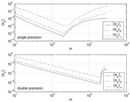
Figure 18: The $L_{1}$-errors (solid), $L_{2}$-errors (dashed) and $L_{\infty}$-errors (dash-dotted) for $\phi$ in (8.4) on $m\times m$ grids, as a function of $m$. Upper panel, single precision; lower panel, double precision.

The accuracy of the method can be characterized by the discrete $L_{1}$, $L_{2}$ and $L_{\infty}$-norms of the errors given in Eq. (7.2). Figure 18 shows these $L_{p}$-norms of the numerical error $e_{\phi}$ of the results obtained with the Fishpak routine on a $(m\times m)$-grid, as a function of $m$, with $A=100$. The upper and lower panel show the error of the single respectively double precision computations. In a similar way we determined the $L_{p}$-norms of the numerical error in the electric field strength $|\tilde{{\boldsymbol{\mathcal{E}}}}|_{ij}$, computed with Eq. (3.19). They are shown in Figure 19.

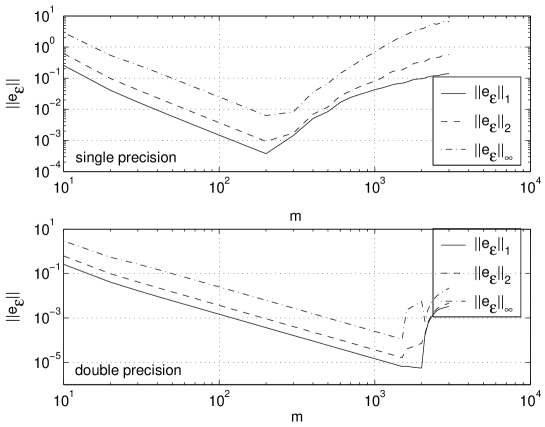
Figure 19: The $L_{1}$-errors (solid), $L_{2}$-errors (dashed) and $L_{\infty}$-errors (dash-dotted) for $|{\boldsymbol{\mathcal{E}}}|$ in Eq. (8.4) on $m\times m$ grids, as a function of $m$. Upper panel, single precision; lower panel, double precision.

Up to a number of grid points of approximately 2000, the errors in the electric potential are of second order, in agreement with the discretization. The errors in the field are also of second order, even though, at first sight, a first-order behavior might be expected, since it’s the derivative of a quantity of second order accuracy. This can be explained through an asymptotic error expansion, which, for simplicity, will be carried in one-dimension. The second order discretization for $\phi$ will give

$$\phi_{j}=\phi(z_{j})+\Delta z^{2}v(z_{j})+O(\Delta z^{4})\,,$$ (8.5)

with a principal error function $v$ which will be smooth if the solution $\phi$ is so. By considering local truncation errors it is seen that $v$ should satisfy $\partial_{zz}v=-\partial_{z}^{4}\phi/12$ with corresponding homogeneous boundary conditions. Then the discretized value of the field at the cell boundary becomes:

$${\mathcal{E}}_{j+\frac{1}{2}}=\frac{\phi_{j}-\phi_{j+1}}{\Delta z}=\frac{\phi(z_{j})-\phi(z_{j+1})}{\Delta z}+\Delta z(v(z_{j})-v(z_{j+1}))+O(\Delta z^{3}),$$ (8.6)

which, using a Taylor expansion around $z_{j+\frac{1}{2}}$, yields

$${\mathcal{E}}_{j+\frac{1}{2}}=-\partial_{z}\phi(z_{j+\frac{1}{2}})+O(\Delta z^{2})-\Delta z^{2}\partial_{z}v(z_{j})+O(\Delta z^{3})={\mathcal{E}}(z_{j+\frac{1}{2}})+O(\Delta z^{2})$$ (8.7)

It is clear that the performance of the Fishpak routine decreases dramatically when more than approximately 2000 grid points (in double precision)are used. We note that these numerical instabilities also show up on a $m_{r}\times m_{z}$ grid if either $m_{r}$ or $m_{z}$ are larger than 2000, approximately, in double precision.

Appendix B: Analytical expressions for the planar front velocity

The asymptotic velocity (5.6) and the convergence towards it can be derived analytically, following arguments in [25]. First, the analysis in [12] shows that a negative streamer front is a pulled front whose dynamics is determined in the leading edge. Linearizing the one-dimensional streamer equations in the leading edge around the field ${\mathcal{E}}_{b}<0$ ahead of the front gives

$$\frac{\partial\sigma}{\partial\tau}={\mathcal{E}}_{b}\frac{\partial\sigma}{\partial z}+D\frac{\partial^{2}\sigma}{\partial z^{2}}+\sigma f(|{\mathcal{E}}_{b}|)\,,$$ (8.8)

where $f(|{\mathcal{E}}_{b}|)=|{\mathcal{E}}_{b}|\exp(-1/|{\mathcal{E}}_{b}|)$. As the nonlinear front region has to be “pulled along” by the evolution of the linear perturbations, the evolution of the linearized equation (8.8) yields an upper bound for the velocity at each instant of time.

For an initial condition of Gaussian form

$$\sigma(z,0)=\sigma_{0}\;\exp\left(-\frac{(z-z_{b})^{2}}{R_{b}^{2}}\right),$$ (8.9)

as used in the paper, the linearized equation (8.8) is solved through

$$\sigma(z,\tau)=\sigma_{0}\;\exp\Big{(}f({\mathcal{E}}_{b})\tau\Big{)}\;\;\;\sqrt{\frac{R_{b}^{2}}{R_{b}^{2}+4D\tau}}\;\exp\left(-\frac{(z-z_{b}+{\mathcal{E}}_{b}\tau)^{2}}{R_{b}^{2}+4D\tau}\right)$$ (8.10)

for all times $\tau\geq 0$. Solving this equation for $z$, the position $z_{f}(\tau)$ of a fixed electron density level $\sigma_{f}$ is

$$\sigma\left(z_{f}(\tau),\tau\right)=\sigma_{f},$$ (8.11)

$$z_{f}^{\pm}(\tau) = z_{b}+|{\mathcal{E}}_{b}|\tau\pm\sqrt{R_{b}^{2}+4D\tau}\,\sqrt{f(|{\mathcal{E}}_{b}|)\tau-\ln\frac{\sigma_{f}}{\sigma_{0}}-\frac{1}{2}\ln\frac{R_{b}^{2}+4D\tau}{R_{b}^{2}}}$$ (8.12)

$$\stackrel{{\scriptstyle\tau\gg 1}}{{\longrightarrow}} z_{b}+\left(|{\mathcal{E}}_{b}|\pm\sqrt{4D\;f(|{\mathcal{E}}_{b}|)}\right)\;\tau+O\left(\sqrt{\tau}\right).$$ (8.13)

For the pulled front moving to the right, we need $z_{f}^{+}(\tau)$. The velocity of the level $\sigma_{f}$ is

$$v_{f}^{lin}(\tau)=\partial_{\tau}z_{f}^{+}(\tau).$$ (8.14)

This equation determines the asymptotic velocity (5.6) that is actually independent of the parameters $\sigma_{0}$, $R_{b}$ and $z_{b}$ of the initial conditions. Moreover the time dependent velocity $v_{f}^{lin}(\tau)$ is an upper bound for the actual velocity $v_{f}(\tau)$ of the full nonlinear problem. The two velocities are compared in Fig. 6.

References

- [1] E. Bazelyan, Y. Raizer, Lightning Physics and Lightning Protection, Institute of Physics Publishing, Bristol, U.K., 2000.
- [2] R. Franz, R. Nemzek, J. Winckler, Television image of a large upward electrical discharge above a thunderstorm system, Science 249 (1990) 48–51.
- [3] D. Sentman, E. Wescott, D. Osborne, M. Heavner, Preliminary results from the Sprites94 campaign: Red sprites, Geophys. Res. Lett. 22 (1995) 1205–1209.
- [4] E. Gerken, U. Inan, C. Barrington-Leigh, Telescopic imaging of sprites, Geophys. Res. Lett. 27 (2000) 2637.
- [5] V. Pasko, M. Stanley, J. Mathews, U. Inan, T. Wood, Electrical discharge from a thundercloud top to the lower ionosphere, Nature 416 (2002) 152–154.
- [6] J. Clements, A. Mizuno, W. Finney, R. Davis, Combined removal of SO2, NOx, and fly ash from simulated flue gas using pulsed streamer corona, IEEE Trans. Ind. Appl. 25 (1989) 62–69.
- [7] E. van Veldhuizen, Electrical Discharges for Environmental Purposes: Fundamentals and Applications, Nova Science Publishers, 2000.
- [8] M. Sato, T. Ohgiyama, J. Clements, Formation of chemical species and their effects on microorganisms using a pulsed high voltage discharge in water, IEEE Trans. Ind. Appl. 32 (1996) 106–112.
- [9] A. Abou-Ghazala, S. Katsuki, K. Schoenbach, F. Dobbs, K. Moreira, Bacterial decontamination of water by means of pulsed-corona discharges, IEEE Trans. Plasma Sci. 30 (2002) 1449–1453.
- [10] S. Nair, A. Pemen, K. Yan, E. van Heesch, K. Ptasinki, A. Drinkenburg, A high temperature pulsed corona plasma system for tar removal from biomass derived fuel gas, J. Electrostatics 61 (2) (2004) 117–127.
- [11] J. Boeuf, Y. Lagmich, L. Pitchford, Electrohydrodynamic force and aerodynamic flow acceleration in surface dielectric barrier discharges, in: Proc. XXVII Int. Conf. Phen. Ion. Gases, Veldhoven, The Netherlands, 2005.
- [12] U. Ebert, W. van Saarloos, C. Caroli, Propagation and structure of planar streamer fronts, Phys. Rev. E 55 (1997) 1530–1549.
- [13] M. Arrayás, U. Ebert, W. Hundsdorfer, Spontaneous branching of anode-directed streamers between planar electrodes, Phys. Rev. Lett. 88 (2002) 174502(1–4).
- [14] A. Rocco, U. Ebert, W. Hundsdorfer, Branching of negative streamers in free flight, Phys. Rev. E 66 (2002) 035102(1–4).
- [15] N. Liu, V. Pasko, Effects of photoionization on propagation and branching of positive and negative streamers in sprites, J. Geophys. Res 109 (2004) A04301(1–17).
- [16] N. Liu, V. Pasko, Effects of photoionization on similarity properties of streamers at various pressures in air, J. Phys. D: Appl. Phys 39 (2006) 327–334.
- [17] M. Arrayás, U. Ebert, Stability of negative ionization fronts: Regularization by electric screening?, Phys. Rev. E 69 (2004) 036214(1–10).
- [18] B. Meulenbroek, A. Rocco, U. Ebert, Streamer branching rationalized by conformal mapping techniques, Phys. Rev. E 69 (2004) 067402(1–4).
- [19] B. Meulenbroek, U. Ebert, L. Schäfer, Regularization of moving boundaries in a Laplacian field by a mixed Dirichlet-Neumann boundary condition – exact results, Phys. Rev. Lett. 95 (2005) 195004.
- [20] U. Ebert, C. Montijn, T. Briels, W. Hundsdorfer, B. Meulenbroek, A. Rocco, E. van Veldhuizen, The multiscale nature of streamers, submitted to Plasma Sources Sci. Technol.
- [21] A. Kulikovsky, The role of the absorption length of photoionizing radiation in streamer dynamics in weak fields: a characteristic scale of ionization domain, J. Phys. D: Appl. Phys. 33 (2000) L5–L7.
- [22] S. Pancheshnyi, S. Starikovskaia, A. Starikovskii, Role of photoionization processes in propagation of cathode-directed streamer, J. Phys. D: Appl. Phys. 34 (2001) 105–115.
- [23] A. Kulikovsky, Comment on “Spontaneous branching of anode-directed streamers between planar electrodes”, Phys. Rev. Lett. 89 (2002) 229401.
- [24] S. Pancheshnyi, A. Starikovskii, Two-dimensional numerical modeling of the cathode-directed streamer development in a long gap at high voltage, J. Phys. D: Appl. Phys. 36 (2003) 2683–2691.
- [25] U. Ebert, W. van Saarloos, Front propagation into unstable states: universal algebraic convergence towards uniformly translating pulled fronts, Physica D 146 (2000) 1–99.
- [26] S. Dhali, P. Williams, Two-dimensional studies of streamers in gases, J. Appl. Phys 62 (1987) 4696–4706.
- [27] Y. Raizer, Gas Discharge Physics, Springer, Berlin, 1991.
- [28] P. Vitello, B. Penetrante, J. Bardsley, Simulation of negative-streamer dynamics in nitrogen, Phys. Rev. E 49 (1994) 5574–5598.
- [29] J. Dutton, A survey of electron swarm data, J. Phys. Chem. Ref. Data 4 (1975) 664.
- [30] E. van Veldhuizen, P. Kemps, W. Rutgers, Streamer branching under influence of the power supply, IEEE Trans. Plasma Sci. 30 (2002) 162–163.
- [31] Y. Bobrov, Y. Yurghelenas, Application of high-resolution schemes in the modeling of ionization waves in gas discharges, Comp. Math. and Math. Physics 38 (1998) 1652–1661.
- [32] W. Hundsdorfer, J. Verwer, Numerical Solution of Time-Dependent Advection-Diffusion-Reaction Equations, Vol. 33 of Series in Comp. Math., Springer, Berlin, 2003.
- [33] M. Barnes, T. Colter, M. Elta, Large-signal time-domain modeling of low-pressure rf glow discharges, J. Appl. Phys. 61 (1986) 81–89.
- [34] J. Blom, R. Trompert, J. Verwer, Algorithm 758: VLUGR2: A vectorizable adaptive grid solver for PDEs in 2D, ACM Trans. Math. Softw. 22 (1996) 302–328.
- [35] S. Gottlieb, C.-W. Shu, E. Tadmor, Strong stability-preserving high-order time discretization methods, SIAM Review 43 (2001) 89–112.
- [36] P. Wesseling, Principles of Computational Fluid Dynamics, Vol. 29 of Series in Comp. Math., Springer, Berlin, 2001.
- [37] U. Schumann, R. Sweet, A direct method for the solution of Poisson’s equation with neumann boundary conditions on a staggered grid of arbitrary size, J. Comp. Phys 20 (1976) 171–182.
- [38] R. Trompert, J. Verwer, A static-regridding method for two-dimensional parabolic partial differential equations, Appl. Numer. Math. 8 (1991) 65–90.
- [39] J. Wackers, A nested-grid finite-difference Poisson solver for concentrated source terms, J. Comp. Appl. Math. 180 (2005) 1–12.
- [40] G. Golub, C. van Loan, Matrix Computations, 3rd Edition, John Hopkins Univ. Press, Baltimore, 1996.
- [41] E. Botta, K. Dekker, Y. Notay, A. van der Ploeg, C. Vuik, F. Wubs, P. de Zeeuw, How fast the Laplace equation was solved in 1995, Appl. Num. Math. 24 (1997) 439–455.
- [42] J. Lang, Adaptive Multilevel Solution of Nonlinear Parabolic PDE Systems. Theory, Algorithm, and Applications, Vol. 16, Springer, 2000.
- [43] P. Colella, M. Dorr, D. Wake, Numerical solution of plasma fluid equations using locally refined grids, J. Comp. Phys 152 (1999) 550–583.
- [44] P. Colella, M. Dorr, D. Wake, A conservative finite difference method for the numerical solution of plasma fluid equations, J. Comp. Phys 149 (1999) 168–193.
- [45] S. Li, L. Petzold, Y. Ren, Stability of moving mesh systems of partial differential equations, SIAM J. Sci. Comp. 20 (1998) 719–738.
- [46] Y. Qui, D. Sloan, Numerical solution of fisher’s equation using a moving mesh method, J. Comp. Phys 146.
-
[47]
C. Montijn, U. Ebert, Avalanche to streamer transition in homogeneous fields,
Tech. Rep. MAS-E0515, CWI,
http://www.cwi.nl/ftp/CWIreports/MAS/MAS-E0515.pdf,
http://www.arxiv.org/pdf/physics/0508109 (2005). - [48] U. Ebert, W. Hundsdorfer, Reply to the comment of A.A. Kulikovsky [23] on “Spontaneous branching of anode-directed streamers between planar electrodes”, Phys. Rev. Lett. 89 (2002) 229402.