Auxiliary-field quantum Monte Carlo calculations of molecular systems
with a Gaussian basis

Abstract

We extend the recently introduced phaseless auxiliary-field quantum Monte Carlo (QMC) approach to any single-particle basis, and apply it to molecular systems with Gaussian basis sets. QMC methods in general scale favorably with system size, as a low power. A QMC approach with auxiliary fields in principle allows an exact solution of the Schrödinger equation in the chosen basis. However, the well-known sign/phase problem causes the statistical noise to increase exponentially. The phaseless method controls this problem by constraining the paths in the auxiliary-field path integrals with an approximate phase condition that depends on a trial wave function. In the present calculations, the trial wave function is a single Slater determinant from a Hartree-Fock calculation. The calculated all-electron total energies show typical systematic errors of no more than a few milli-Hartrees compared to exact results. At equilibrium geometries in the molecules we studied, this accuracy is roughly comparable to that of coupled-cluster with single and double excitations and with non-iterative triples, CCSD(T). For stretched bonds in H₂O, our method exhibits better overall accuracy and a more uniform behavior than CCSD(T).

I Introduction

Obtaining the solution of the Schrödinger equation, even within a finite Hilbert space, is an important goal in quantum chemistry and in condensed matter physics, both in its own right and for calibrating approximate methods. In quantum chemistry, a variety of approaches have been developed over the last fifty years, which range in quality from the mean-field Hartree-Fock (HF) to the exact full configuration interaction (FCI) solution. In between these two limits, a hierarchy of approximations have been developed which improve upon the Hartree-Fock solution at the expense of increasing computational cost qc_ref .

The FCI method is quite formidable computationally, because its cost grows exponentially with the number of electrons and basis functions. Recently, the density matrix renormalization group (DMRG) approach was introduced as a method to potentially obtain near-FCI quality solutions of the Schrödinger equation for quantum chemical Hamiltonians white_1 ; dmrg_H2O_41 ; dmrg_rev . The results so far are promising. For example, DMRG was applied recently dmrg_H2O_41 to study the water molecule using a double-zeta atomic-natural-orbital (ANO) basis (41 basis functions), which is currently intractable with FCI.

Among the approximate approaches, coupled cluster (CC) methods have been the most successful, especially at equilibrium geometries ccsdt_ref ; ccsdt_crawford . However, standard CC methods are non-variational and their computational cost grows rather steeply with the system size as well. For example, the most popular among them, CC with single and double excitations and with non-iterative triples [CCSD(T)], has an $N^{7}$ scaling with the size of the basis.

Quantum Monte Carlo (QMC) methods are an attractive means for a non-perturbative and explicit treatment of the interacting many-fermion system. These methods tend to have favorable scaling with system size, often as a low power. The most established QMC method, the real space fixed-node diffusion Monte Carlo (DMC) method, has been applied successfully to calculate many properties of solids QMC_rmp and molecules QMC_rev_mole .

Recently, an alternative and complementary QMC method has been introduced zhang_krakauer for realistic electronic Hamiltonians, based on a field-theoretic approach with auxiliary fields. The central idea of auxiliary-field (AF) QMC methods is the mapping of the interacting many-body problem into a linear combination of non-interacting problems coupled to external AFs. Averaging over different AF configurations is performed by Monte Carlo techniques. The basic formalism of AF QMC methods has mostly been applied to lattice models of strongly interacting systems BSS ; Koonin . In these models, the simplified form of the two-body interactions makes possible an efficient mapping with real AFs. As a result, “only” a sign problem Zhang_review occurs. Constrained path methods Zhang ; Zhang_review have been developed to approximately control the sign problem, which have been shown to be quite accurate.

The potential of AF QMC methods for realistic Hamiltonians has long been recognized and pursued Silvestrelli93 ; shiftcont_rom97 ; Wilson95 . However, wide and general applications were not realized because of a lack of control for the phase problem. Except for special cases, the two-body electronic interactions lead to complex AFs. The many-dimensional integration over complex variables in turn leads to an exponentially increasing noise and therefore breakdown of the method. The phaseless AF QMC method zhang_krakauer was introduced to control the phase problem in an approximate manner.

In Ref. zhang_krakauer , a general framework was developed on how to use importance sampling of the determinants to deal with the complex phase. An approximate constraint was then formulated with a trial wave function to constrain the paths in AF space and eliminate the growth of noise. Because of the constraint, the calculated ground state energy is no longer exact and is not variational. In applications to several $sp$-bonded materials zhang_krakauer ; zhang_krakauer2 ; cherry , it was shown that the method, with a plane-wave basis and simple trial wave functions, gave accurate results for systems from simple atoms to large supercells. The phaseless AF QMC method was also recently applied to the strongly correlated transition metal oxide molecules TiO and MnO alsaidi , again yielding results in good agreement with experiment using simple mean-field trial wave functions.

The success of the phaseless AF approach in solid-state applications with plane-waves has motivated us to extend it to a generic one-particle basis, targeting in particular quantum chemistry problems. Applying the new AF QMC method to such problems is very appealing, especially with the integral role basis sets play in quantum chemistry methods. This method allows QMC calculations using any choice of one-particle basis. It provides a framework for general many-body calculations which can import straightforwardly many of the well-established technologies from more traditional approaches. By importance-sampled random walks, the phaseless AF QMC method obtains the many-body ground state with an ensemble of loosely coupled independent-particle calculations which propagate with imaginary-time. The ground-state wave function is represented by a linear combination of non-orthogonal Slater determinants.

In this paper we report the first results from this effort. We discuss aspects of the new method when implemented with Gaussian basis sets. We present benchmark results on $sp$-bonded atoms and molecules. All-electron total energies are calculated for various first-row atoms and molecules, and compared with FCI and DMRG results where available or with CCSD(T) otherwise. The behavior of the method is also studied as a function of basis size, including an ANO basis roos ; roos_footnote1 in H₂O and O₂, each with $92$ basis functions. We then test the method away from equilibrium geometries, calculating the equilibrium bond length and also stretching the bonds in the water molecule by a factor between $1$ and $8$ within a cc-pVDZ basis cc_basis . In all our calculations the trial wave function is taken to be a single Slater determinant from Hartree-Fock, either restricted (RHF) or unrestricted (UHF). Their effect on the accuracy is examined. The calculated energies with the optimal HF wave function typically show systematic errors of no more than a few milli-Hartree (mE_h) compared to exact results. For stretched bonds in H₂O, our method exhibits better overall accuracy and more uniform behavior than CCSD(T).

An additional benefit of the present AF QMC implementation is its value for algorithmic studies. Compared to the plane-wave algorithm, the generic basis AF QMC method typically has much more effective basis sets. As a result, the basis size is often much smaller and the method is significantly cheaper computationally. Further, direct comparisons can be more easily made between the QMC results and those obtained with more established correlated methods, as indicated above. Extra ingredients such as pseudopotentials can be removed, with the only remaining uncertainty being the systematic error from the phaseless approximation. In this study, we take advantage of this feature to make detailed benchmark studies of the systematic error.

The rest of the paper is organized as follows. The phaseless AF QMC method is first briefly reviewed in the next section. We then describe its implementation with the Gaussian basis in Sec. III, together with some results to illustrate the behavior and characteristics of this approach. Section IV gives some of the details of the computational procedures. In Sec. V and Sec. VI, we present the results of our calculations, including calculations of the H₂O molecule both at the equilibrium geometry and with stretched bond lengths, and total energies and energy differences (binding, ionization, and electron affinity) for various other first-row atoms and diatomic molecules. Finally in Sec. VII we make concluding remarks, together with a brief discussion of possibilities for further improvement of the new algorithm.

II Formalism

The full electronic Hamiltonian for a many-fermion system with two-body interactions can be written in any orthonormal one-particle basis in the general form

$${\hat{H}}={\hat{H}_{1}}+{\hat{H}_{2}}=\sum_{i,j}^{N}{T_{ij}c_{i}^{\dagger}c_{j}}+{1\over 2}\sum_{i,j,k,l}^{N}{V_{ijkl}c_{i}^{\dagger}c_{j}^{\dagger}c_{k}c_{l}},$$ (1)

where $N$ is the size of the chosen one-particle basis, and $c_{i}^{\dagger}$ and $c_{i}$ are the corresponding creation and annihilation operators. Both the one-body ($T_{ij}$) and two-body ($V_{ijkl}$) matrix elements are known.

The auxiliary-field quantum Monte Carlo method obtains the ground state $\left|\Psi_{G}\right\rangle$ of ${\hat{H}}$, by projecting from a trial wave function $\left|\Psi_{T}\right\rangle$ using the imaginary-time propagator $e^{-\tau{\hat{H}}}$:

$$\left|\Psi_{G}\right\rangle\propto\lim_{n\to\infty}(e^{-\tau{\hat{H}}})^{n}\left|\Psi_{T}\right\rangle.$$ (2)

The trial wave function $\left|\Psi_{T}\right\rangle$, which should have a non zero overlap with the exact ground state, is assumed to be in the form of a single determinant or a linear combination of Slater determinants.

The timestep, $\tau$, is chosen to be small enough so that ${\hat{H}_{1}}$ and ${\hat{H}_{2}}$ in the propagator can be accurately separated with the Trotter decomposition:

$$e^{-\tau{\hat{H}}}=e^{-\tau{\hat{H}_{1}}/2}e^{-\tau{\hat{H}_{2}}}e^{-\tau{\hat{H}_{1}}/2}+{\cal{O}}(\tau^{3}).$$ (3)

The action of the propagator $e^{-\tau{\hat{H}_{1}}}$ on a Slater determinant yields another determinant. This is not the case with $e^{-\tau{\hat{H}_{2}}}$, which however can be written as an integral of one-body operators using a Hubbard-Stratonovich (HS) transformation HS :

$$e^{-\tau{\hat{H}_{2}}}=\prod_{\alpha}\Bigg{(}{1\over\sqrt{2\pi}}\int_{-\infty}^{\infty}d\sigma_{\alpha}\,e^{-\frac{1}{2}\sigma_{\alpha}^{2}}e^{\sqrt{\tau}\,\sigma_{\alpha}\,\sqrt{\zeta_{\alpha}}\,{\hat{v}_{\alpha}}}\Bigg{)},$$ (4)

where the one-body operators ${\hat{v}_{\alpha}}$ can be defined generally for any two-body operator by writing the latter in a quadratic form, such as ${\hat{H}_{2}}=-{1\over 2}\sum_{\alpha}\zeta_{\alpha}{\hat{v}_{\alpha}}^{2}$, with $\zeta_{\alpha}$ a real number. Monte Carlo methods are very efficient at evaluating multi-dimensional integrals as in Eq. (4). For example, the projection of Eq. (2) can be realized iteratively: An ensemble of Slater determinants $\{\,|\phi\rangle\,\}$ are initialized to the trial wave function $|\Psi_{T}\rangle$, which are then propagated to a new ensemble $\{\,|\phi^{\prime}\rangle\,\}$ using $e^{-\tau{\hat{H}}}$ of Eq. (3), and so on, until convergence is reached. For each Slater determinant in the ensemble, the two-body part in Eq. (4) can be applied stochastically by sampling an AF configuration, $\{\,\sigma_{\alpha}\,\}$. In the standard AF QMC approach, the projection is often done Zhang_review as a path integral with paths of fixed length in imaginary time, using a Metropolis or heat-bath algorithm.

This straightforward approach, however, will generally lead to an exponential increase in the statistical fluctuations with the projection time. The source of the fluctuations is that the one-body operators $\hat{\mathbf{v}}\equiv\{\,{\hat{v}_{\alpha}}\,\}$ are generally complex, since usually $\zeta_{\alpha}$ cannot all be made positive in Eq. (4). As a result, the orbitals in $|\phi\rangle$ will become complex as the projection proceeds. For large projection time, the phase of each $|\phi\rangle$ becomes random, and the MC representation of $|\Psi_{G}\rangle$ becomes dominated by noise. This leads to the phase problem and the divergence of the fluctuations. The phase problem is of the same origin as the sign problem that occurs when the one-body operators $\hat{\mathbf{v}}$ are real, but is more severe because for each $|\phi\rangle$, instead of a $+|\phi\rangle$ and $-|\phi\rangle$ symmetry Zhang , there is now an infinite set $\{e^{i\theta}|\phi\rangle,\theta\in[0,2\pi)\}$ among which the Monte Carlo sampling cannot distinguish.

We used the phaseless auxiliary-field QMC method to control the phase problem. In order to implement a phaseless constraint, the method recasts the imaginary-time path integral as a branching random walk in Slater-determinant space Zhang ; zhang_krakauer . It uses a trial wave function $|\Psi_{T}\rangle$ and a complex importance function, $\langle\Psi_{T}|\phi\rangle$, to construct phaseless random walkers, $|\phi\rangle/\langle\Psi_{T}|\phi\rangle$, which are invariant under a phase gauge transformation. The resulting two-dimensional diffusion process in the complex plane of the overlap $\langle\Psi_{T}|\phi\rangle$ is then approximated as a diffusion process in one dimension.

As mentioned earlier, the ground-state energy computed with the so-called mixed estimate is approximate and not variational in the phaseless method. The error depends on $|\Psi_{T}\rangle$, vanishing when $|\Psi_{T}\rangle$ is exact. This is the only error in the method that cannot be eliminated systematically. The method has been applied to atoms, molecules, and simple solids, using a plane-wave basis and pseudopotentials, and has proved very successful zhang_krakauer ; zhang_krakauer2 ; alsaidi .

III Implementation using a localized basis

With Gaussian basis sets, the matrix elements of interest to QMC and the overlap matrix can be imported from quantum chemistry programs. It is more convenient to use orthonormal basis functions, which ensure the usual commutation relations of the creation and destruction operators. To set up the Hamiltonian in Eq. (1), we first transform the non-orthogonal basis into an orthogonalized basis set. The one- and two-body matrix elements, $T_{ij}$ and $V_{ijkl}$, are then expressed with respect to this basis via the transformation, based on the original matrix elements.

To carry out the HS transformation of Eq. (4), we first map the two-body interaction matrix $V_{ijkl}$ into a real, symmetric supermatrix ${\cal{V}}_{\mu[i,l],\nu[j,k]}$ where $\mu,\nu=1,\ldots,N^{2}$. This is then expressed in terms of its eigenvalues $(-\lambda_{\alpha})$ and eigenvectors $X_{\mu}^{\alpha}$: ${\cal{V}_{\mu,\nu}}=-\sum_{\alpha}\lambda_{\alpha}X_{\mu}^{\alpha}\,X_{\nu}^{\alpha}$.

The two-body operator ${\hat{H}}_{2}$ of Eq. (1) can be written as the sum of a one-body operator ${\hat{H}}^{\prime}_{1}$ and a two-body operator ${\hat{H}}^{\prime}_{2}$. The latter can be further expressed in terms of the eigenvectors of ${\cal{V}}_{\mu,\nu}$ as

$${\hat{H}^{\prime}}_{2}=-\frac{1}{2}\,\sum_{\alpha}\lambda_{\alpha}{\hat{v}^{2}}_{\alpha},$$ (5)

where the one-body operator ${\hat{v}}_{\alpha}$ is,

$${\hat{v}}_{\alpha}=\sum_{i,l}X_{\mu[i,l]}^{\alpha}a^{{\dagger}}_{i}a_{l}.$$ (6)

Note that ${\hat{v}^{\dagger}}_{\alpha}={\hat{v}}_{\alpha}$ for real basis functions, as is the case here. The form in Eq. (5) is now amenable to the HS transformation of Eq. (4).

In this case the number of the HS fields is equal to the number of non-zero eigenvalues $(-\lambda_{\alpha})$ of the symmetrized two-body supermatrix. Other forms of decomposition and HS transformation are possible, and their efficiency and effectiveness with a constraint can vary.(For example, using a modified Cholesky decomposition will eliminate the need to diagonalize the supermatrix and potentially reduces the computational cost of synthesizing the matrix. However, this will generally lead to a larger number of HS fields, and hence increase the QMC computational cost.) We will defer further analysis of this freedom to a future publication.

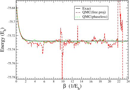
Figure 1: The projection of the ground state of H₂O/STO-6G. Starting from the HF trial wave function, the total energy is plotted vs. the projection time $\beta=n\,\tau$, as obtained using the free projection QMC (exact but suffers from the phase problem) and the phaseless approximation. For comparison, we show also the exact projection which is obtained form diagonalization of the many-body Hamiltonian. The phaseless QMC method tracks smoothly the exact projection with no sign of the uncontrolled fluctuations in free projection.

To illustrate the method, we use the H₂O molecule in a minimal STO-6G basis. This problem is small enough to permit detailed comparison with exact diagonalization. Starting from HF solution, the projection in Eq. (2) was applied using: i) the exact many-body propagator $e^{-\tau\hat{H}}$ acting on the wave function expanded in terms of the exact eigenstates of the many-body Hamiltonian ${\hat{H}}$, ii) the free projection QMC method (no constraint imposed) which is exact but suffers from the phase problem, and iii) the phaseless QMC which is approximate but controls the phase problem. Figure 1 plots the results of total-energy mixed-estimator zhang_krakauer , corresponding to these three calculations. Up to a projection time of $\beta~{}\approx~{}2$ E${}_{h}^{-1}$, both QMC methods show essentially the same convergence of the total-energy. For large projection times, the free-projection starts showing the phase problem in the form of large fluctuations. Around $\beta~{}\approx~{}23$ E${}_{h}^{-1}$ these fluctuations diverge on the scale of the plot. For larger number of particles or larger basis sets, this divergence would have occurred at much earlier projection times $\beta$. The phaseless QMC method, by contrast, follows the exact projection with finite variance as the random walk proceeds.

In our implementation, we found it advantageous to first subtract the mean-field “background” from ${\hat{v}}_{\alpha}$ before applying the Hubbard-Stratonovich transformation. In this case, Eq. (5) is replaced by,

$${\hat{H}}^{\prime}_{2}=-\frac{1}{2}\sum_{\alpha}\lambda_{\alpha}({\hat{v}}_{\alpha}-\langle{\hat{v}}_{\alpha}\rangle)^{2}+{\hat{H}^{\prime\prime}}_{1},$$ (7)

where $\langle{\hat{v}}_{\alpha}\rangle=\langle\Psi_{T}|{\hat{v}}_{\alpha}|\Psi_{T}\rangle$ and ${\hat{H}^{\prime\prime}}_{1}$ is the one-body operator:

$${\hat{H}^{\prime\prime}}_{1}=-\frac{1}{2}\,\sum_{\alpha}\left({\hat{v}}_{\alpha}\langle{\hat{v}}_{\alpha}\rangle+{\hat{v}}_{\alpha}\langle{\hat{v}}_{\alpha}\rangle-\langle{\hat{v}}_{\alpha}\rangle\langle{\hat{v}}_{\alpha}\rangle\right).$$ (8)

Equations (5) and (7) are equivalent. When the approximate phaseless projection is imposed, however, using Eq. (7) before applying the HS transformation leads to an improved behavior.

We illustrate this point in Fig. 2. Using the same STO-6G minimal basis, we plot the Trotter time-step convergence of the total energy of the H₂O molecule, calculated with the HS transformations of Eq. (5) and Eq. (7), for both the phaseless QMC method and for (exact) free-projection. For comparison, the ground state energy obtained from exact diagonalization is also shown. The Trotter extrapolated QMC energy (see inset of Fig. 2) is $-75.72725(4)$ E_h with the HS decomposition of Eq. (5) and $-75.72849(5)$ E_h with Eq. (7). Monte Carlo statistical error bars are on the last digit and are shown in parentheses. For comparison, the exact ground-state energy is $-75.72799$ E_h.

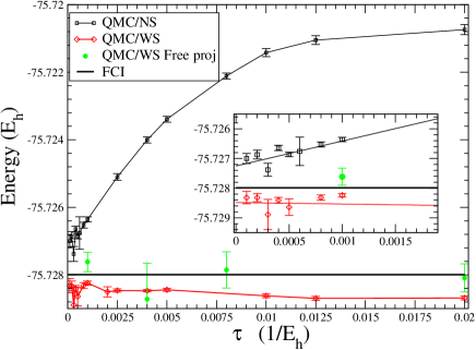
Figure 2: QMC Trotter time-step dependence. The total energy of the H₂O/STO-6G molecule from phaseless QMC is shown vs. the time-step size $\tau$, using the HS transformations of Eq. (5) (labeled as QMC/NS) and of Eq. (7) (labeled as QMC/WS, in which the mean-field “background” is subtracted). Results from free-projection (exact but suffers from the phase problem) are also shown, together with that of the exact FCI. Points are connected by straight lines for clarity. The insert shows a closer look at small values of $\tau$, together with linear fits of the QMC data.

Similar results and analysis have also been presented in phaseless AF QMC calculations in boson systems Wirawan05 . We comment that the issue in Fig. 2 is different from the shifted contour approach shiftcont_rom97 , dispite formal similarities. With the importance sampling scheme of Ref. zhang_krakauer , Eqs. (5) and (7) would both be exact and give the same results under free projection, since the mean-field shift is automatically applied via the importance sampling transformation regardless of which form of ${\hat{H}}^{\prime}_{2}$ is used Wirawan04 . The different behaviors discussed above arise only because of the imposition of the phase projection to one-dimension zhang_krakauer , in which the substraction of the mean-field background helps to reduce the “rotation” of the random walkers in the complex $\langle\Psi_{T}|\phi\rangle$-plane and thus the severity of the projection.

IV Computational Details

We apply our method to several atomic and molecular systems, which were chosen primarily for benchmarking purposes and which have all been previously studied using well-established correlated methods such as coupled cluster (CC), full configuration interaction (FCI), or density matrix renormalization group (DMRG) methods. In these and in our QMC calculations, the core and valence electrons are fully correlated.

All the QMC calculations reported below used a single Hartree-Fock Slater determinant as the trial wave function. For all systems, QMC was done with the best variational single determinant, namely the unrestricted Hartree-Fock (UHF) solution. In addition, we have also tested the restricted Hartree-Fock (RHF) solution as the trial wave function in some cases. No additional optimization or tuning of the trial wave function was performed beyond the mean-field Hartree-Fock calculation.

The QMC code is interfaced with GAMESSgamess and NWChemnwchem to import the Gaussian one-electron and two-electron matrix elements, the overlap matrix, and the trial wave function. All of our calculations are done using the spherical harmonics representation of basis functions.

We performed the FCI calculations using MOLPRO molpro ; fci_molpro and the coupled cluster calcuations using NWChem nwchem . Unless otherwise noted, the coupled cluster calculations for atoms and molecules with a singlet state are of the type RHF-RCCSD(T) i.e. based on the RHF reference state, while those for a multiplet state are of the unrestricted type, UHF-UCCSD(T) based on the UHF solution.

Table 1: The binding energy (BE) of H₂O calculated with four basis sets: STO-6G, cc-pVDZ, and double- and triple-zeta ANO roos_footnote1 . Also shown are all-electron total energies for O, H, and H₂O. Monte Carlo statistical errors are in the last digit and are shown in parentheses. All energies are in Hartrees. The FCI value for H₂O/cc-pVDZ is from Ref. H2O_Olsen , while the DMRG energy of H2O and the FCI energy of O within the double-zeta ANO are from Ref. dmrg_H2O_41 .

	UHF	CCSD(T)	FCI/DMRG	QMC
STO-6G
H	-0.471 039	-0.471 039	-0.471 039	-0.471 039
O	-74.516 816	-74.516 816	-74.516 816	-74.516 816
H2O	-75.676 506	-75.727 931	-75.727 991	-75.728 5(1)
BE	0.217 612	0.269 037	0.269 097	0.269 5(1)
cc-pVDZ
H	-0.499 278	-0.499 278	-0.499 278	-0.499 278
O	-74.792 166	-74.911 552	-74.911 744	-74.909 6(1)
H2O	-76.024 039	-76.241 201	-76.241 860	-76.242 4(2)
BE	0.233 317	0.331 093	0.331 560	0.334 3(2)
DZ ANO
H	-0.499 944	-0.499 944	-0.499 944	-0.499 944
O	-74.816 273	-74.961 956	-74.962 350	-74.959 6(1)
H2O	-76.057 621	-76.314 141	-76.314 715	-76.316 3(6)
BE	0.241 460	0.352 959	0.352 477	0.356 8(7)
TZ ANO
H	-0.499 973	-0.499 973		-0.499 973
O	-74.818 648	-75.000 129		-74.997 0(4)
H2O	-76.060 589	-76.367 528		-76.370(1)
BE	0.241 995	0.367 453		0.373(1)

V Equilibrium Geometries

As a first test of our method, we calculate in this section total energies and binding energies for some well-studied systems at their equilibrium geometries. The first subsection contains results for the water molecule in the vicinity of the equilibrium structure and the O₂ dimer at equilibrium bond length. The second subsection contains results for other first-row atoms and diatomic molecules, including total ground-state energies, binding energy, convergence with basis sets, atomic ionization potentials, and electron affinities. In the next section, we test the method by studying bond stretching of the water molecule.

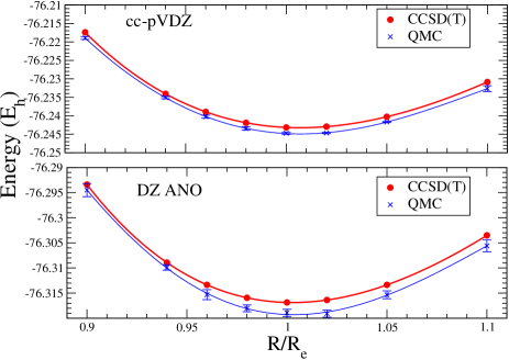
Figure 3: Calculation of the equilibrium bond length of H₂O within the cc-pVDZ basis and DZ ANO basis, using CCSD(T) and the present QMC method. All-electron total energies (in Hartrees) are shown as a function of the O-H bond length (in units of the experimental equilibrium value, $R_{e}$), with the angle between the two O-H bonds fixed at the experimental value. Monte Carlo statistical error bars are indicated. The lines are based on a polynomial fit to the data.

V.1 H₂O and O₂

The water molecule has a long benchmarking history saxe ; Bauschlicher ; H2O_Olsen ; H2O_DMC ; dmrg_H2O_41 . Table 1 presents results calculated by HF, CCSD(T), FCI, and the present QMC method. We show the all-electron total energies of the individual atoms H and O, and the total and binding energies of H₂O. Four different basis sets were used: minimal STO-6G, cc-pVDZ cc_basis , and the double zeta (DZ) and triple-zeta (TZ) ANO bases of Widmark, Malmqvist, and Roos roos ; roos_footnote1 . For H₂O, these have 7, 24, 41, and 92 basis functions, respectively. The H₂O geometries were as follows: results using the minimal STO-6G correspond to positions (in Bohr) of O$(0,0,0)$ and H$(0,\pm 1.515263,-1.058898)$ with $C_{2v}$ symmetry, while the cc-pVDZ results used the geometry of Ref. H2O_Olsen . The DZ ANO and TZ ANO results were obtained with the geometry given in Ref. dmrg_H2O_41 .

The QMC calculations used UHF trial wave functions. (For H₂O, the RHF and UHF solutions are identical at the equilibrium bond length.) The FCI total energies of H₂O/cc-pVDZ are those of Ref. H2O_Olsen . FCI results for H₂O are not within reach for the DZ ANO basis, but DMRG results are available from a recent study dmrg_H2O_41 , which are shown under FCI. The FCI energy of O/DZ ANO is also from Ref. dmrg_H2O_41 . Neither FCI nor DMRG is within reach presently for the TZ ANO basis.

Table 2: Binding energy (BE) of O₂ using cc-pVDZ, double- and triple-zeta ANO roos_footnote1 basis sets. The calculated all-electron total energies are also shown. The experimental bond length of $R_{e}=1.2074$ Å  was used. O atom results are in Table 1. Monte Carlo statistical errors are in the last digit and are shown in parentheses. All energies are in Hartrees.

	UHF	UCCSD(T)	QMC
cc-pVDZ
O2	-149.627 780	-149.989 319	-149.982 6(3)
BE	0.043 448	0.166 215	0.163 5(3)
DZ ANO
O2	-149.679 669	-150.095 668	-150.090 7(6)
BE	0.047 123	0.171 756	0.171 5(7)
TZ ANO
O2	-149.689 251	-150.187 965	-150.186(2)
BE	0.051 955	0.187 706	0.192(2)

Table 3: The calculated all-electron total energies of various first-row atoms and diatomic molecules in their ground states. We show the RHF, UHF, CCSD(T) energies, and the FCI results where available. The basis set and the number of basis functions are shown in the third column. Our QMC results based on the RHF and UHF trial wave functions are shown in two columns. MC statistical errors are in the last digit and shown in parentheses. For completeness, we show in the last column some of the available estimated experimental, non-relativistic, infinite nuclear mass energy (i.e., the estimated exact result at the infinite basis size limit). All energies are in Hartrees.

	Re(Å)	basis(#)	RHF	UHF	CCSD(T)	FCI	QMC/RHF	QMC/UHF	E${}_{\rm{est}}^{\infty}$
H2	0.741	cc-pVDZ(10)	$-$1.128 714		$-$1.163 411	$-$1.163 411	$-$1.163 60(1)		$-$1.174 4
Li		cc-pVDZ(14)		$-$7.432 421	$-$7.432 638	$-$7.432 638		$-$7.432 633(3)	$-$7.478 1
Li2	2.673	cc-pVDZ(28)	$-$14.869 499	$-$14.870 128	$-$14.901 386	$-$14.901 392	$-$14.902 5(1)	$-$14.900 35(9)	$-$14.995 4
Be		cc-pVDZ(14)	$-$14.572 338	$-$14.572 611	$-$14.617 407	$-$14.617 409	$-$14.617 26(7)	$-$14.617 63(8)	$-$14.667 4
Be2	2.45	cc-pVDZ(28)	$-$29.132 211	$-$29.154 535	$-$29.234 246		$-$29.231 3(2)	$-$29.234 1(2)	$-$29.338 5
Be		cc-pVTZ(30)	$-$14.572 874	$-$14.573 183	$-$14.623 790	$-$14.623 810	$-$14.622 4(2)	$-$14.622 8(2)	$-$14.667 4
Be2	2.45	cc-pVTZ(60)	$-$29.133 688	$-$29.156 165	$-$29.253 734		$-$29.248 8(5)	$-$29.251 1(3)	$-$29.338 5
N		cc-pVDZ(14)		$-$54.391 115	$-$54.479 944	$-$54.480 115		$-$54.479 56(7)	$-$54.589 3
N2	1.094	cc-pVDZ(28)	$-$108.954 553		$-$109.278 722		$-$109.281 6(3)		$-$109.542 3
F		cc-pVDZ(14)		$-$99.375 240	$-$99.529 322	$-$99.529 518		$-$99.528 1(3)	$-$99.734
F2	1.412	cc-pVDZ(28)	$-$198.685 670	$-$198.695 746	$-$199.101 151		$-$199.100 3(5)	$-$199.102 4(4)
BH	1.256	cc-pVDZ(19)	$-$25.125 188	$-$25.131 227	$-$25.215 917	$-$25.216 401	$-$25.217 5(3)	$-$25.215 1(2)
CH+	1.146	cc-pVDZ(19)	$-$37.900 480	$-$37.909 823	$-$38.003 207	$-$38.003 712	$-$38.006 9(3)	$-$38.000 5(4)
NH	1.056	cc-pVDZ(19)		$-$54.966 091	$-$55.093 298	$-$55.093 721		$-$55.093 18(7)
OH+	1.032	6$-$31G∗∗(19)		$-$74.973 345	$-$75.093 371			$-$75.093 08(9)
HF	0.920	cc-pVDZ(19)	$-$100.019 280		$-$100.230 098		$-$100.231 2(1)

We see that the agreement between the QMC, CCSD(T), and FCI results is quite good. As mentioned, the calculated ground-state energies in the present phaseless QMC method are not variational, which can be seen in the results in H₂O, for example. QMC binding energy results of H₂O overestimate the exact values by $0.4(1)$, $2.7(2)$, $4.4(6)$ mE_h, for the STO-6G, cc-pVDZ, and DZ ANO basis, respectively. The CCSD(T) method, which is highly accurate at this geometry, has errors of $0.06$, $0.47$, $0.48$ mE_h, respectively. In the TZ ANO basis, CCSD(T) and QMC yield binding energies of 0.3675 and 0.373(1) E_h, respectively.

As mentioned, the DZ ANO and TZ ANO calculations of H₂O were for the geometry in Ref. dmrg_H2O_41 . Using CCSD(T), we verified that the experimental H₂O geometry would lower the molecular total energy by 2.7 mE_h and 4.0 mE_h for the two basis sets. This would increase the binding energy by the same amount, and bring the CCSD(T) binding energy with the TZ ANO basis to good agreement with 0.370 E_h, the basis extrapolated value of Feller and Peterson Feller_Peterson . For comparison, the experimental binding energy of H₂O is $0.3707$ E_h (with the zero-point energy removed) Feller_Peterson .

Figure 3 shows a comparison of QMC and CCSD(T) results in the vicinity of the H₂O equilibrium bond length, using cc-pVDZ and ANO double zeta basis sets. The angle between the two O-H bonds is fixed at the experimental angle of 104.4798 degrees, and we varied $R/R_{e}$ where $R_{e}=1.81$ Bohr is the experimental bond length H2O_ref_exp . For the cc-pVDZ basis, the CCSD(T) and QMC equilibrium bond lengths calculated from these curves are 1.007 R_e and 1.007(2) R_e, respectively. The corresponding values using the ANO DZ basis set are 1.003 R_e and 1.006(4) R_e.

Table 4: The first ionization potential of first-row elements as calculated in the cc-pVDZ and cc-pVTZ basis sets. For selected elements, additional cc-pVQZ and cc-pV5Z basis sets are also used. We show the values obtained using HF, CCSD(T), and QMC, together with experimental results ion_book ; andersen_ion . QMC statistical errors are in the last digit and are shown in parentheses. All energies are in eV.

Atom	HF	CCSD(T)	QMC	Exp
cc-pVDZ
Li	$5.342$	$5.345$	$5.345(1)$	$5.39$
Be	$8.079$	$9.290$	$9.296(2)$	$9.32$
B	$8.038$	$8.066$	$7.942(5)$	$8.30$
C	$10.803$	$10.983$	$11.025(5)$	$11.26$
O	$11.965$	$12.853$	$12.808(2)$	$13.62$
N	$13.895$	$14.195$	$14.306(3)$	$14.53$
F	$15.640$	$16.710$	$16.725(8)$	$17.42$
Ne	$19.668$	$20.893$	$20.948(5)$	$21.56$
cc-pVTZ
Li	$5.342$	$5.353$	$5.353(1)$	$5.39$
Be	$8.045$	$9.285$	$9.259(7)$	$9.32$
B	$8.038$	$8.228$	$8.08(1)$	$8.30$
C	$10.798$	$11.184$	$11.237(8)$	$11.26$
O	$12.011$	$13.326$	$13.256(7)$	$13.62$
N	$13.892$	$14.449$	$14.574(4)$	$14.53$
F	$15.654$	$17.142$	$17.154(7)$	$17.42$
Ne	$19.673$	$21.309$	$21.37(1)$	$21.56$
cc-pVQZ
B	$8.041$	$8.260$	$8.19(5)$	$8.30$
O	$12.018$	$13.493$	$13.44(1)$	$13.62$
F	$15.649$	$17.314$	$17.33(2)$	$17.42$
Ne	$19.661$	$21.488$	$21.57(2)$	$21.56$
cc-pV5Z
O	$12.022$	$13.558$	$13.50(1)$	$13.62$

Table 5: Same as Table 4, but for the electron affinity and using the aug-cc-pVDZ and aug-cc-pVTZ basis sets aug_cc_basis .

Atom	HF	CCSD(T)	QMC	Exp
aug-cc-pVDZ
B	$-0.300$	$0.172$	$0.125(5)$	$0.28$
C	$0.468$	$1.145$	$1.205(6)$	$1.263$
O	$-0.523$	$1.189$	$1.25(1)$	$1.46$
N	$-1.858$	$-0.512$	$-0.52(1)$	$-0.07(2)$
F	$1.284$	$3.228$	$3.40(1)$	$3.4$
Ne	$-7.724$	$-7.321$	$-7.32(1)$
aug-cc-pVTZ
B	$-0.305$	$0.235$	$0.23(4)$	$0.28$
C	$0.453$	$1.226$	$1.29(3)$	$1.263$
O	$-0.565$	$1.336$	$1.40(5)$	$1.46$
N	$-1.813$	$-0.296$	$-0.28(3)$	$-0.07(2)$
F	$1.195$	$3.317$	$3.59(4)$	$3.4$
Ne	$-6.479$	$-6.108$	$-6.30(7)$

We present results for the O₂ molecule in Table 2. The experimental equilibrium bond length of $R_{e}=1.2074$ Å  is used for all of these calculations. Results are shown for the three larger basis sets used in the above H₂O calculations. These include the cc-pVDZ and the DZ and TZ ANO basis sets, which give 28, 46, and 92 basis functions for O₂, respectively. QMC and CCSD(T) results are again in good agreement. In the TZ ANO basis, the CCSD(T) and QMC binding energies are 0.188 and 0.192(2) E_h, respectively. Our QMC value is in excellent agreement with our previous binding energy 0.191(4) calculated using pseudopotentials and planewaves alsaidi . Also for comparison, the basis extrapolated binding energy at the CCSD(T) level is 0.191 E_h and the experimental value is 0.192 E_h (with the zero-point energy removed) Feller_Peterson .

V.2 First-row atoms and diatomic molecules

V.2.1 All-electron total ground-state energies

In Table 3, we show the total energies of various first-row atoms and diatomic molecules at the equilibrium geometry as calculated using RHF, UHF, CCSD(T), and also the FCI energies where available. For reference, we show also some available E${}_{\rm{est}}^{\infty}$, the estimated experimental non relativistic, infinite nuclear mass energy kolos_roothan ; davidson_est_enyergy ; filippi_umrigar . These represent the estimated exact results at the infinite basis size limit, and are thus significantly lower than the CCSD(T), FCI, or QMC energies because of the small basis size chosen in these benchmark calculations.

For singlets where both RHF and UHF solutions exist, QMC calculations were done with each as a trial wave function, and both results are shown in Table 3. In such cases, QMC with the best variational single Slater determinant as trial wave function, namely QMC/UHF, appears to always give better energy values. We discuss this effect further in Sec.VI with stretched bonds in H₂O.

Our QMC energies are generally within a few mE_h of the FCI or the CCSD(T) energies. It is interesting to note the cases of the berylium atom and molecule. The Be atom, which has a near $2s$-$2p$ degeneracy, has often been used as a benchmark in Green’s function or diffusion Monte Carlo (DMC) studies Umrigar_DMC ; Casula_geminal . Optimized Slater-Jastrow trial wave functions with a single determinant are known to lead to significant errors, of $\sim 10$ mE_h, in the calculated fixed-node ground-state energy Umrigar_DMC . (This error is largely removed when multi-determinant trial wave functions are used to account for the near degeneracy. For example, DMC with an optimized Slater-Jastrow trial wave function using four determinants is extremely accurate Umrigar_DMC .) In the present QMC method, the phaseless approximation using a single Slater determinant appears to be significantly less dependent on the trial wave function, with systematic errors of $\sim 1$ mE_h or less. Of course, the DMC calculations work in real configuration space and thus have the advantage of no finite-basis errors. Measured as a fraction of the correlation energy, the present QMC/UHF still has a substantially smaller systematic error, of about 2 Be/cc-pVTZ.

Correspondingly, the Be₂ dimer is a notorious case in quantum chemistry Martin_CPL . A DMC calculation using optimized single-determinant trial wave functions did not obtain binding Schautz_Be2-98 . Our QMC/UHF total energies are within $\sim 2$ mE_h of CCSD(T), and the resulting binding energy with the larger cc-pVTZ basis is $5.5(4)$ mE_h, in good agreement with the CCSD(T) value of $6.1$ mE_h. The finite basis-size errors are still significant at this basis size — at the CCSD(T) level, the binding energy is $3.6$ mE_h with the cc-pVQZ basis and $4.2$ mE_h with the cc-pV5Z basis. Thus a more detailed study is necessary before a direct and definitive comparison can be made between QMC and experiment (BE: $4.0$ mE_h). The QMC result is consistent with the previous calculation using a plane-wave basis zhang_krakauer , which should be at the infinite basis limit (aside from pseudopotential errors).

V.2.2 Ionization potentials and electron affinities

In Tables 4 and 5 we present a summary of the calculated first ionization potential and electron affinity for first-row elements. For the ionization energy study, we used the cc-pVDZ and cc-pVTZ double- and triple-zeta basis sets cc_basis for all the elements. A few selected elements are then studied, using the larger cc-pVQZ basis sets. Also we looked at O with a cc-pV5Z basis set with 91 basis functions. For the electron affinity we used the aug-cc-pVDZ and aug-cc-pVTZ sets aug_cc_basis . For comparison, we show the values calculated using HF, CCSD(T), and QMC, as well as the experimental data from Refs. ion_book ; andersen_ion .

The agreement between QMC and the coupled cluster CCSD(T) results is in general very good. For unstable or meta-stable negative ions (N^- and Ne^-), the Hamiltonian expressed with a localized basis always yields an atomic-like ground state. In Tables 4 and 5, the total ground-state energies are not shown, but the mean difference between the QMC and CCSD(T) values among all the atoms and ions is less than 3 mE_h. The negative charged F ion, F^-/aug-cc-pVTZ, has the largest discrepancy of $\sim 7$ mE_h. An MCSCF study nwchem showed that the RHF single determinant gives a rather poor description of the ion.

Table 6: Basis-size and trial wave function dependence in stretched-bond calculations in H₂O. Equilibrium geometries are the same as in Table. I. The all-electron total energy of H₂O is shown using three different basis sets: minimal STO-6G, cc-pVDZ, and DZ ANO roos_footnote1 with 7, 24, and 41 bases functions, respectively. The O-H bond lengths are stretched to $1.5\,R_{e}$ and $2\,R_{e}$. QMC energies obtained with both RHF and UHF trial wave functions are shown in the last two columns. Statistical errors in QMC are in the last digit, and are shown in parentheses. FCI/DMRG results are from the same sources as in Table 1. All energies are in Hartrees.

bond length	RHF	UHF	CCSD(T)	FCI	QMC/RHF	QMC/UHF
STO-6G
$1.5\,R_{e}$	-75.440 432	-75.502 069		-75.600 039	-75.576 8(3)	-75.596 5(6)
$2\,R_{e}$	-75.141 587	-75.464 541		-75.486 528	-75.355 7(3)	-75.488 0(3)
cc-pVDZ
$1.5\,R_{e}$	-75.802 387	-75.829 813	-76.070 717	-76.072 348	-76.068 8(3)	-76.069 7(2)
$2\,R_{e}$	-75.587 711	-75.793 668	-75.955 485	-75.951 665	-75.897 3(4)	-75.954 6(2)
DZ ANO
$1.5\,R_{e}$	-75.817 273	-75.852 670	-76.129 442	-76.131 050	-76.126 5(7)	-76.129 0(5)
$2\,R_{e}$	-75.602 850	-75.818 969	-76.009 395		-75.950(1)	-76.011(1)

VI H₂O bond stretching

We next examine the accuracy of our method in describing bond stretching. The ability of a computational method to deliver uniform accuracy as bonds are stretched/broken is obviously important in chemistry. It also provides an indicator for the potential accuracy of a method for solids, mimicking different levels of electron correlation. Our method uses a trial wave function in the constraint to deal with the phase problem. Almost all calculations to date, both with the plane-wave basis and in the present study, have used single Slater determinant trial wave functions. Since the quality of such wave functions decreases as bonds are stretched and correlation effects become more important, it is a significant challenge for the method to maintain its quality and obtain uniformly accurate results.

We apply our method to stretched bonds in H₂O, which has served as an excellent benchmark system H2O_Olsen ; dmrg_H2O_41 . Symmetric O-H bond length stretching is studied. The bond angle between the two O-H bonds is held fixed, while the O-H bond length is increased from its equilibrium value. We considered three different basis sets: STO-6G, cc-pVDZ cc_basis , and DZ ANO roos . For the small basis, we used the same geometry as in Table I. For the two larger basis sets, we used the same geometries as those of Ref. H2O_Olsen and Ref. dmrg_H2O_41 for comparison with their FCI and DMRG energies, respectively.

The results are shown in Table 6. In addition to QMC/UHF, i.e., using the variationally optimal HF solution as the trial wave function, we also carried out QMC calculations using the RHF solution, in order to further examine the effect of the trial wave function. As bonds are stretched, static correlation becomes increasingly important. The RHF solution becomes inceasingly unfavorable compared to the UHF solution, which has the correct behavior in the dissociation limit. As can be seen in Table 6, QMC with the RHF trial wave function (QMC/RHF) performs worse than QMC/UHF, which is consistent with the trend seen in Table 3. Indeed, the QMC/RHF results deterioate as the bonds are stretched, reflecting the qualitatively incorrect nature of the RHF trial wave function at large bond lengths.

In the range of bond lengths in Table 6, QMC with the UHF trial wave function gives roughly comparable accuracy as CCSD(T). For example, in the cc-pVDZ basis at $1.5\,R_{e}$, QMC/UHF over-estimates the energy by 2.7(1) mE_h, while CCSD(T) over-estimates it by 1.6 mE_h. At $2\,R_{e}$, both QMC/UHF and CCSD(T) under-estimate the energy, by 3.0(2) and 3.8 mE_h, respectively. In the DZ ANO basis for $1.5~{}R_{e}$, QMC/UHF is above the DMRG value by $2.1(5)$ mE_h, while CCSD(T) is above by $1.6$ mE_h.

Larger bond stretching of up to 8 R_e is presented in Figure 4, using the cc-pVDZ valence double-zeta basis. QMC results are compared with exact FCI H2O_Olsen and with coupled cluster results using RHF and UHF reference states (CCSD(T) and UCCSD(T), respectively). The inset shows the errors of the various methods from the FCI numbers. CCSD(T) is excellent near equilibrium, but is much worse at large bond lengths. (As mentioned, QMC with RHF trial wave functions would show similar behavior at large bond lengths.) UCCSD(T) performs much better for larger bond lengths, but is worse in the intermediate regime with errors larger than $10$ mE_h. Our QMC results are in good agreement with the exact energies, showing a maximum discrepancy of about 4(1) mE_h, which occurs at $8R_{e}$. Together with the equilibrium results, the method is seen to yield rather uniform accuracy across these bond lengths. This is encouraging, given that it is achieved with the same choice, namely the variational UHF solution, as the trial wave function throughout the entire region.

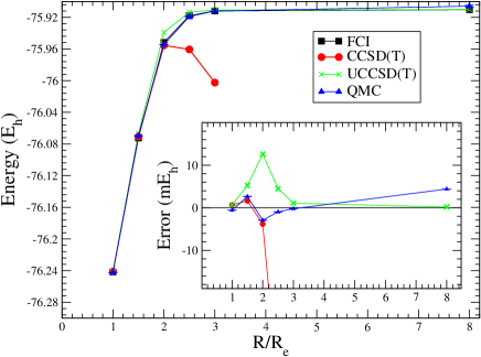
Figure 4: A comparison of bond stretching in H₂O/cc-pVDZ between the present QMC, coupled cluster methods, and FCI H2O_Olsen . The main graph shows the calculated total energy (in Hartrees) as a function of the O-H bond length. The inset shows the errors (in milli-Hartrees) of various methods with respect to FCI. Points are connected by straight lines for clarity. QMC statistical error bars are shown.

VII Discussion and Summary

The present QMC method provides an approximate, but non-perturbative approach for many-electron calculations. It can directly incorporate traditional electronic-structure machinery, such as high-quality basis sets, effective-core potentials, etc. The method obtains the many-body ground state by building a stochastic linear superposition of non-orthogonal independent-particle solutions. Thus, algorithmically it shares many of the ingredients in more standard methods in quantum chemistry and solid state physics. Its computational cost scales with the number of basis functions as $N^{3}$ to $N^{4}$.

The accuracy of the present QMC method depends on the reference or trial wave function $\left|\Psi_{T}\right\rangle$, which in this study is chosen as the HF state. As in coupled cluster methods, the trial wave function is the starting point of the ground-state projection, but in QMC all excitations are implicitly included by the projection. Errors arise from the phaseless approximation in the projection, which uses $|\Psi_{T}\rangle$ to approximate the phase of the contribution of a Slater determinant to the ground state, via the importance-sampling transformation.

We have found, as shown in Tables 3 and 6, that the most accurate energies are in general obtained using the best variational single determinant $|\Psi_{T}\rangle$. This is simply the HF solution when RHF and UHF are the same (e.g., in the H₂O molecule at equilibrium), and is the UHF solution when the two differ. In the latter case, the method seems relatively insensitive, within the unrestricted framework, to whether a Hartree-Fock or hybrid B3LYP Slater determinant is used.

In contrast to the diffusion Monte Carlo (DMC) method, the present QMC must deal with finite basis-set errors and basis-size convergence. However, the ability to use any single-particle basis can also be advantageous. For example, in addition to the connection to quantum chemistry methods, our new method also makes possible QMC calculations for general model Hamiltonians, which are frequently used in the study of correlated electron systems. Like the present AF QMC method, DMC is also approximate, using a trial wave function to impose the fixed-node approximation to control the sign problem. The trial wave functions that have been used in our method are much simpler. Because of the complementary nature of the two different methods, direct comparisons are not always straightforward. Indications from the current calculations and earlier plane-wave studies are that the systematic accuracy of the phaseless approximation compare favorably with fixed-node DMC.

In summary, we extended the recently introduced phaseless QMC method to handle any one-particle basis, and applied it to atoms and molecules using Gaussian basis sets. Overall, our results at and near the equilibrium geometries are roughly comparable to those obtained using CCSD(T), but are superior for bond stretching. Our preliminary results (to be published elsewhere) on bond-breaking in several diatomic molecules show similar uniform accuracy. For a first application, these results are quite encouraging. There are many possibilities for further improvement of the method. Currently, we are investigating different forms of Hubbard-Stratonovich transformations, possibilities for better scaling, as well as applications of the present method in transition metal oxides and other systems.

VIII Acknowledgments:

We would like to thank E. J. Walter and S. R. White for useful discussions. This work is supported by ONR (N000149710049, N000140110365, and N000140510055), NSF (DMR-0535529), and ARO (48752PH) grants, and by the DOE computational materials science network (CMSN). Computations were carried out at the Center for Piezoelectrics by Design, the SciClone Cluster at the College of William and Mary, NCSA at UIUC, and SDSC at UCSD.

References

- (1) A. Szabo and N. S. Ostlund, Modern Quantum Chemistry (McGraw-Hill, New York, 1989).
- (2) S. R. White and R. L. Martin, J. Chem. Phys. 110, 4127 (1999).
- (3) Garnet Kin-Lic Chan and Martin Head-Gordon, J. Chem. Phys. 118, 8551 (2003).
- (4) U. Schollwöck, Rev. Mod. Phys. 77, 259 (2005).
- (5) J. Cizek, J. Chem. Phys. 45, 4256 (1966).
- (6) T. Crawford and H. Schaefer, Rev. Comp. Chem. 14, 33 (2000).
- (7) W. M. C. Foulkes, L. Mitas, R. J. Needs, and G. Rajagopal, Rev. Mod. Phys. 71, 33 (2001).
- (8) D. M. Ceperley and L. Mitas, in New Methods in Computational Quantum Mechanics Advances in Chemical Physics, XCIII, eds. I. Prigogine and S. A. Rice, 1996; B. L. Hammond, W. A. Lester, Jr. and P. J. Reynolds, Monte Carlo methods in ab initio quantum chemistry (World Scientific, Singapore, 1994).
- (9) Shiwei Zhang and Henry Krakauer, Phys. Rev. Lett. 90, 136401 (2003).
- (10) R. Blankenbecler, D. J. Scalapino, and R. L. Sugar, Phys. Rev. D 24, 2278 (1981).
- (11) G. Sugiyama and S. E. Koonin, Ann. Phys. (NY) 168, 1 (1986).
- (12) Shiwei Zhang, in Theoretical Methods for Strongly Correlated Electrons, ed. by D. Senechal, A.-M. Tremblay, and C. Bourbonnais (Springer 2003).
- (13) Shiwei Zhang, J. Carlson, and J. E. Gubernatis, Phys. Rev. B 55, 7464 (1997).
- (14) P. L. Silvestrelli, S. Baroni, and R. Car, Phys. Rev. Lett. 71, 1148 (1993).
- (15) Naomi Rom, D. M. Charutz, and Daniel Neuhauser, Chem. Phys. Lett. 270, 382 (1997).
- (16) M. T. Wilson and B. L. Gyorffy, J. Phys. Condens. Matter 7, 371 (1995).
- (17) Shiwei Zhang, Henry Krakauer, Wissam Al-Saidi, and Malliga Suewattana, Comp. Phys. Comm. 169, 394 (2005).
- (18) Malliga Suewattana et. al.(in preparation).
- (19) W. A. Al-Saidi, Henry Krakauer, and Shiwei Zhang, Phys. Rev. B 73, 075103 (2006).
- (20) P. O. Widmark, P. A. Malmqvist, and B. Roos, Theo. Chim. Acta, 77, 291 (1990).
- (21) Basis sets can be obtained from the Extensible Computational Chemistry Environment Basis Set Database (http://www.emsl.pnl.gov/forms/basisform.html). The ANO basis sets used for H2O and O2 are designated “Roos Augmented Double Zeta ANO” and “Roos Augmented Triple Zeta ANO.”
- (22) Thom H. Dunning, J. Chem. Phys. 90, 1007 (1989).
- (23) R. L. Stratonovich, Sov. Phys. Dokl. 2, 416 (1958); J. Hubbard, Phys. Rev. Lett. 3, 77 (1959).
- (24) Wirawan Purwanto and Shiwei Zhang, Phys. Rev. A 72, 053610 (2005).
- (25) Wirawan Purwanto and Shiwei Zhang, Phys. Rev. E 70, 056702 (2004).
- (26) M. W. Schmidt, K. K. Baldridge, J. A. Boatz, S. T. Ebert, M. S. Gordon, J. H. Jensen, S. Koseki, N. Matsunaga, K. A. Nguyen, S. J. Su, T. L. Windus, M. Dupuis, and J. A. Montgomery, J. Comput. Chem. 14, 1347 (1993); http://www.msg.ameslab.gov/GAMESS/GAMESS.html.
- (27) T. P. Straatsma, E. Aprá, T. L. Windus, E. J. Bylaska, W. de Jong, S. Hirata, M. Valiev, M. T. Hackler, L. Pollack, R. J. Harrison, M. Dupuis, D. M. A. Smith, J. Nieplocha, V. Tipparaju, M. Krishnan, A. A. Auer, E. Brown, G. Cisneros, G. I. Fann, H. Fruchtl, J. Garza, K. Hirao, R. Kendall, J. A. Nichols, K. Tsemekhman, K. Wolinski, J. Anchell, D. Bernholdt, P. Borowski, T. Clark, D. Clerc, H. Dachsel, M. Deegan, K. Dyall, D. Elwood, E. Glendening, M. Gutowski, A. Hess, J. Jaffe, B. Johnson, J. Ju, R. Kobayashi, R. Kutteh, Z. Lin, R. Littlefield, X. Long, B. Meng, T. Nakajima, S. Niu, M. Rosing, G. Sandrone, M. Stave, H. Taylor, G. Thomas, J. van Lenthe, A. Wong, and Z. Zhang, ”NWChem, A Computational Chemistry Package for Parallel Computers, Version 4.6” (2004), Pacific Northwest National Laboratory, Richland, Washington 99352-0999, USA.
- (28) MOLPRO version 2002.6 is a package of ab initio programs written by H.-J. Werner and P. J. Knowles, with contributions from J. Almlof, R. D. Amos, M. J. O. Deegan, S. T. Elbert, C. Hampel, W. Meyer, K. A. Peterson, R. M. Pitzer, ¨ A. J. Stone, P. R. Taylor, and R. Lindh, Universitat Bielefeld, Bielefeld, Germany, University of Sussex, Falmer, Brighton, England, 1996.
- (29) P. J. Knowles and N. C. Handy, Chem. Phys. Letters 111, 315 (1984); P. J. Knowles and N. C. Handy, Comp. Phys. Commun. 54, 75 (1989).
- (30) P. Saxe, H. F. Schaefer III, and N. C. Handy, Chem. Phys. Lett. 79, 202 (1981).
- (31) C. W. Bauschlicher and P. R. Taylor, J. Chem. Phys. 85, 2779 (1986).
- (32) J. Olsen, P. Jorgensen, H. Koch, A. Balkova, and R. J. Bartlett, J. Chem. Phys. 104, 8007 (1995).
- (33) A. Luchow, J. B. Anderson, and D. Feller, J. Chem. Phys. 106, 7706 (1997).
- (34) D. Feller and K. A. Peterson, J. Chem. Phys. 110, 8384 (1999).
- (35) A. R. Hoy and P. R. Bunker, J. Molecular Structure 74, 1, (1979).
- (36) W. Kolos and C. C. J. Roothaan, Rev. Mod. Phys. 32, 219 (1960).
- (37) Ernest R. Davidson, Stanley A. Hagstrom, Subhas J. Chakravorty, Verena Meiser Umar, and Charlotte Froese Fischer, Phys. Rev. A 44, 7071 (1991).
- (38) Claudia Filippi and C. J. Umrigar, J. Chem. Phys. 105, 213 (1996).
- (39) Micah L. Abrams and C. David Sherrill, J. Chem. Phys. 118, 1604 (2003).
- (40) C. J. Umrigar, M. P. Nightingale, and K. J. Runge, J. Chem. Phys. 99, 2865 (1993).
- (41) M. Casula and S. Sorella, J. Chem. Phys. 119, 6500 (2003).
- (42) Jan M. L. Martin, Chem. Phys. Lett. 303, 399(1999).
- (43) F. Schautz, H.-J. Flad, and M. Dolg, Theor. Chem. Acc. 99, 231 (1998).
- (44) A. A. Radzig and B. M. Smirnov, Reference data on atoms, molecules, and ions (Springer-Verlag, 1985).
- (45) T. Andersen, H. K. Haugen, and H. Hotop, J. Phys. Chem. Ref. Data 28, 1511 (1999).
- (46) Rick A. Kendall, Thom H. Dunning, Jr., and Robert J. Harrison, J. Chem. Phys. 96, 6796 (1992).