Geometric optics of whispering gallery modes

Abstract

Quasiclassical approach and geometric optics allow to describe rather accurately whispering gallery modes in convex axisymmetric bodies. Using this approach we obtain practical formulas for the calculation of eigenfrequencies and radiative Q-factors in dielectrical spheroid and compare them with the known solutions for the particular cases and with numerical calculations. We show how geometrical interpretation allows expansion of the method on arbitrary shaped axisymmetric bodies.

1 Introduction

Submillimeter size optical microspheres made of fused silica with whispering gallery modes (WGM)[1] can have extremely high quality-factor, up to $10^{10}$ that makes them promising devices for applications in optoelectronics and experimental physics. Historically Richtmyer[2] was the first to suggest that whispering gallery modes in axisymmetric dielectric body should have very high quality-factor. He examined the cases of sphere and torus. However only recent breakthroughs in technology in several labs allowed producing not only spherical and not only fused silica but spheroidal, toroidal [3, 4] or even arbitrary form axisymmetrical optical microcavities from crystalline materials preserving or even increasing high quality factor [5]. Especially interesting are devices manufactured of nonlinear optical crystals. Microresonators of this type can be used as high-finesse cavities for laser stabilization, as frequency discriminators and high-sensitive displacement sensors, as sensors of ambient medium and in optoelectronical RF high-stable oscillators. (See for example materials of the special LEOS workshop on WGM microresonators [6]).

The theory of WGMs in microspheres is well established and allows precise calculation of eigenmodes, radiative losses and field distribution both analytically and numerically. Unfortunately, the situation changes drastically even in the case of simplest axisymmetrical geometry, different from ideal sphere or cylinder. No closed analytical solution can be found in this case. Direct numerical methods like finite elements method are also inefficient when the size of a cavity is several orders larger than the wavelength. The theory of quasiclassical methods of eigenfrequencies approximation starting from pioneering paper by Keller and Rubinow have made a great progress lately [8]. For the practical evaluation of precision that these methods can in principal provide, we chose a practical problem of calculation of eigenfrequencies in dielectric spheroid and found a series over angular mode number $l$. This choice of geometry is convenient due to several reasons: 1) other shapes, for example toroids [4] may be approximated by equivalent spheroids; 2) the eikonal equation as well as scalar Helmholtz equation (but not the vector one!) is separable in spheroidal coordinates that gives additional flexibility in understanding quasiclassical methods and comparing them with other approximations; 3) in the limit of zero eccentricity spheroid turns to sphere for which exact solution and series over $l$ up to $l^{-8/3}$ is known [9].

The Helmholtz vector equation is unseparable [10] in spheroidal coordinates and no vector harmonics tangential to the surface of spheroid can be build. That is why there are no pure TE or TM modes in spheroids but only hybrid ones. Different methods of separation of variables (SVM) using series expansions with either spheroidal or spherical functions have been proposed [11, 12, 13]. Unfortunately they lead to extremely bulky infinite sets of equations which can be solved numerically only in simplest cases and the convergence is not proved. Exact characteristic equation for the eigenfrequencies in dielectric spheroid was suggested[14] without provement that if real could significantly ease the task of finding eigenfrequencies. However, we can not confirm this claim as this characteristic equation contradicts limiting cases with the known solutions i.e. ideal sphere and axisymmetrical oscillations in a spheroid with perfectly conducting walls [15].

Nevertheless, in case of whispering gallery modes adjacent to equatorial plane the energy is mostly concentrated in tangential or normal to the surface electric components that can be treated as quasi-TE or quasi-TM modes and analyzed with good approximation using scalar wave equations.

Using quasiclassical method we deduce below the following practical approximation for the eigenfrequencies of whispering gallery modes in spheroid:

$$nka = l+\alpha_{q}\left(\frac{l}{2}\right)^{1/3}+\frac{2p(a-b)+a}{2b}-\frac{\chi n}{\sqrt{n^{2}-1}}+\frac{3\alpha_{q}^{2}}{20}\left(\frac{l}{2}\right)^{-1/3}$$ (1)

$$+ \frac{\alpha_{q}}{12}\left(\frac{2p(a^{3}-b^{3})+a^{3}}{b^{3}}+\frac{2n^{3}\chi(2\chi^{2}-3)}{(n^{2}-1)^{3/2}}\right)\left(\frac{l}{2}\right)^{-2/3}+O(l^{-1}),$$

where $a$ and $b$ are equatorial and polar semiaxises, $k=\frac{\lambda}{2\pi}$ is the wavenumber, $l\gg 1$, $p=l-|m|=0,1,2,$… and $q=1,2,3,$… are integer mode indices, $\alpha_{q}$ are the $q$-th roots of the equation $Ai(-\alpha_{q})=0$ ($Ai(z)$ is the Airy function), $n$ is refraction index of a spheroid and $\chi=1$ for quasi-TE and $\chi=1/n^{2}$ for quasi-TM modes.

2 Spheroidal coordinate system

There are several equivalent ways to introduce prolate and oblate spheroidal coordinates and corresponding eigenfunctions [16, 17, 18]. The following widely used system of coordinates allows to analyze prolate and oblate geometries simultaneously:

$$x=\frac{d}{2}[(\xi^{2}-s)(1-\eta^{2})]^{1/2}\cos(\phi)$$

$$y=\frac{d}{2}[(\xi^{2}-s)(1-\eta^{2})]^{1/2}\sin(\phi)$$

$$z=\frac{d}{2}\xi\eta,$$ (2)

where we have introduced a sign variable $s$ which is equal to 1 for the prolate geometry with $\xi\in[1,\infty)$ determining spheroids and $\eta\in[-1,1]$ describing two-sheeted hyperboloids of revolution (Fig.1, right). Consequently, $s=-1$ gives oblate spheroids for $\xi\in[0,\infty)$ and one-sheeted hyperboloids of revolution (Fig.1, right). $d/2$ is the semidistance between focal points. We are interested in the modes inside a spheroid adjacent to its surface in the equatorial plane. It is convenient to designate a semiaxis in this plane as $a$ and in the $z$-axis of rotational symmetry of the body as $b$. In this case $d^{2}/4=s(b^{2}-a^{2})$ and eccentricity $\varepsilon=\sqrt{1-(a/b)^{2s}}$.

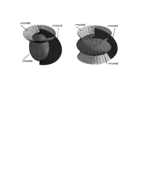
Figure 1: Graphical representation of prolate and oblate spheroidal coordinate systems ($\xi,~{}\eta,~{}\phi$).

The scalar Helmholtz differential equation

$$\frac{\partial}{\partial\xi}(\xi^{2}-s)\frac{\partial}{\partial\xi}\Psi+\frac{\partial}{\partial\eta}(1-\eta^{2})\frac{\partial}{\partial\eta}\Psi+\left(c^{2}(\xi^{2}\mp\eta^{2})-\frac{m^{2}}{1-\eta^{2}}-s\frac{m^{2}}{\xi^{2}-s}\right)\Psi=0,$$ (3)

where $c=kd/2$ is separable. The solution is $\Psi=R_{ml}(c,\xi)S_{ml}(c,\eta)e^{im\phi}$ where radial and angular functions are determined by the following equations:

$$\frac{\partial}{\partial\xi}(\xi^{2}-s)\frac{\partial R}{\partial\xi}-\left(\lambda_{ml}-c^{2}\xi^{2}+s\frac{m^{2}}{\xi^{2}-s}\right)R=0,$$ (4)

$$\frac{\partial}{\partial\eta}(1-\eta^{2})\frac{\partial S}{\partial\eta}+\left(\lambda_{ml}-sc^{2}\eta^{2}-\frac{m^{2}}{1-\eta^{2}}\right)S=0.$$ (5)

Here $\lambda_{ml}$ is the separation constant of the equations which should be independently determined and it is a function on $m$, $l$ and $c$. With substitution $\xi=2r/d$ the first equation transforms to the equation for the spherical Bessel function $j_{l}(kr)$ if $d/2\to 0$ in which case the second equation immediately turns to the equation for the associated Legendre polynomials $P_{m}^{l}(\eta)$ with $\lambda_{m,l}=l(l+1)$. That is why spheroidal functions are frequently analyzed as decomposition over these spherical functions.

The calculation of spheroidal functions and of $\lambda_{ml}$ is not a trivial task [19, 20]. The approximation of spheroidal functions and their zeros may seem more straightforward for the calculation of eigenfrequencies of spheroids, however we found that another approach that we develop below gives better results and may be easily generalized to other geometries.

3 Eikonal approximation in spheroid

The eikonal approximation is a powerful method for solving optical problems in inhomogeneous media where the scale of the variations is much larger than the wavelength. It was shown by Keller and Rubinow [7] that it can also be applied to eigenfrequency problems and that it has very clear quasiclassical ray interpretation. It is important that this quasiclassical ray interpretation requiring simple calculation of the ray paths along the geodesic surfaces and application of phase equality (quantum) conditions gives precisely the same equations as the eikonal equations. Eikonal equations allow, however, to obtain more easily not only eigenfrequencies but field distribution also.

In the eikonal approximation the solution of the Helmholtz scalar equation is found as a superposition of straight rays:

$$u({\bf r})=A({\bf r})e^{\imath k_{0}S({\bf r})}.$$ (6)

The first order approximation for the phase function $S$ called eikonal is determined by the following equation.

$$(\nabla S)^{2}=\epsilon({\bf r}),$$ (7)

where $\epsilon$ is optical susceptibility. For our problem of searching for eigenfrequencies $\epsilon$ does not depend on coordinates, $\epsilon=n^{2}$ inside the cavity and $\epsilon=1$ – outside. Though the eikonal can be found as complex rays in the external area and stitched on the boundary as well as ray method of Keller and Rubinow [7, 8, 21] can be extended for whispering gallery modes in dielectrical bodies in a more simple way [22]. To do so we must account for an additional phase shift on the dielectric boundary. Fresnel amplitude coefficient of reflection [23]:

$${\cal R}=\frac{\chi n\cos\theta-i\sqrt{n^{2}\sin^{2}\theta-1}}{\chi n\cos\theta+i\sqrt{n^{2}\sin^{2}\theta-1}},$$ (8)

gives the following approximations for the phase shift for grazing angles:

$$i\ln{\cal R} = \,\pi-\Phi_{r}$$

$$\simeq \,\pi-\frac{2\chi n}{\sqrt{n^{2}-1}}\cos\theta-\frac{\chi n^{3}(3-2\chi^{2})}{3(n^{2}-1)^{3/2}}\cos^{3}\theta-\frac{\chi n^{5}(15-20\chi^{2}+8\chi^{4})}{20(n^{2}-1)^{5/2}}\cos^{5}\theta+O(\cos^{7}\theta).$$

Nevertheless, direct use of this phase shift in the equations for internal rays as suggested in [22] leads to incorrect results. The reason is a well known Goos-Hänchen effect – the shift of the reflected beam along the surface. The beams behave as if they are reflected from a fixious surface hold away from the real boundary at $\sigma_{r}=\frac{\Phi_{r}}{2kn\cos\theta}$. That is why we may substitute the problem for a dielectric body with the problem for an equivalent body enlarged on $\sigma_{r}$ with the totally reflecting boundaries. The parameters of equivalent spheroid are marked below with overbars.

The eikonal equation separates in spheroidal coordinates if we choose $S=S_{1}(\xi)+S_{2}(\eta)+S_{3}(\phi)$:

$$\frac{\xi^{2}-s}{\xi^{2}-s\eta^{2}}\left(\frac{\partial S_{1}(\xi)}{\partial\xi}\right)^{2}+\frac{1-\eta^{2}}{\xi^{2}-s\eta^{2}}\left(\frac{\partial S_{2}(\eta)}{\partial\eta}\right)^{2}+\frac{1}{(\xi^{2}-s)(1-\eta^{2})}\left(\frac{\partial S_{3}(\phi)}{\partial\phi}\right)^{2}=\frac{n^{2}d^{2}}{4}.$$ (10)

After immediate separation of $\left(\frac{\partial S}{\partial\phi}\right)=\mu$ we have:

$$(\xi^{2}-s)\left(\frac{\partial S_{1}(\xi)}{\partial\xi}\right)^{2}+(1-\eta^{2})\left(\frac{\partial S_{2}(\eta)}{\partial\eta}\right)^{2}+\frac{s\mu^{2}}{\xi^{2}-s}+\frac{\mu^{2}}{1-\eta^{2}}-\frac{n^{2}d^{2}}{4}(\xi^{2}-s\eta^{2})=0.$$ (11)

Introducing another separation constant $\nu$ we finally obtain solutions:

$$\frac{\partial S_{1}(\xi)}{\partial\xi}=\left(\frac{n^{2}d^{2}\xi^{2}}{4(\xi^{2}-s)}-\frac{\nu^{2}}{\xi^{2}-s}-\frac{s\mu^{2}}{(\xi^{2}-s)^{2}}\right)^{1/2},$$

$$\frac{\partial S_{2}(\eta)}{\partial\eta}=\left(\frac{\nu^{2}}{1-\eta^{2}}-\frac{n^{2}d^{2}s\eta^{2}}{4(1-\eta^{2})}-\frac{\mu^{2}}{(1-\eta^{2})^{2}}\right)^{1/2},$$ (12)

which after some manipulations transform to:

$$\frac{\partial S_{1}(\xi)}{\partial\xi}=\frac{nd}{2}\frac{\sqrt{(\xi^{2}-\xi_{c}^{2})(\xi^{2}-s\eta_{c}^{2})}}{\xi^{2}-s}$$

$$\frac{\partial S_{2}(\eta)}{\partial\eta}=\frac{nd}{2}\frac{\sqrt{(\eta_{c}^{2}-\eta^{2})(\xi_{c}^{2}-s\eta^{2})}}{1-\eta^{2}}$$

$$\frac{\partial S_{3}(\phi)}{\partial\phi}=\mu,$$ (13)

where

$$\eta_{c}^{2} = \frac{(1+s\alpha)-\sqrt{(1+s\alpha)^{2}-4s\alpha\eta^{2}_{0}}}{2s\alpha}$$

$$\xi_{c}^{2} = \frac{(1+s\alpha)+\sqrt{(1+s\alpha)^{2}-4s\alpha\eta^{2}_{0}}}{2\alpha}=\frac{1+s\alpha}{\alpha}-s\eta^{2}_{c},$$ (14)

where $\alpha=\frac{n^{2}d^{2}}{4\nu^{2}}$, $\eta^{2}_{0}=1-\mu^{2}/\nu^{2}$. It is now the time to turn to the quasiclassical ray interpretation [7, 8, 29, 30, 31] of whispering gallery modes. The eikonal equation describes rays spreading inside a cavity along straight lines and reflecting from boundaries. For the whispering gallery modes the angle of reflection is close to $\pi/2$. The envelope of these rays forms a caustic surface which in case of spheroid is also a spheroid determined by a parameter $\xi_{c}$. The rays are the tangents to this internal caustic spheroid and follow along eodesic lines on it. In case of ideal sphere all the rays of the same family lie in the same plane. However, even a slightest eccentricity removes this degeneracy and inclined closed circular modes which should be more accurately called quasimodes [24] are turned into open-ended helices winding up on caustic spheroid precessing [25], and filling up the whole region as in a clew. The upper and lower points of these trajectories determine another caustic surface with a parameter $\eta_{c}$ determining two-sheeted hyperboloid for prolate or one-sheeted hyperboloid for oblate spheroid. The value of $\eta_{c}$ has very simple mechanical interpretation. The rays in the eikonal approximation are equivalent to the trajectories of a point-like billiard ball inside the cavity. As axisymmetrical surface can not change the angular momentum related to the $z$ axis, it should be conserved on the ray ($L_{z}\equiv\rho^{2}\dot{\phi}=const$, $\rho^{2}=x^{2}+y^{2}$) as well as the kinetic energy (velocity). That is why $\eta_{c}$ is simply equal to the sine of the angle between the equatorial plane and the trajectory crossing the equator and at the same time it determines the maximum elongation of the trajectory from the equator plane. Together with the simple law of reflection on the boundaries (angle of reflectance is equal to the angle of incidence i.e normal component is reversed at reflection [30] $\dot{\bf r}_{r}=\dot{\bf i}_{r}-2{\vec{\sigma}}({\vec{\sigma}}\dot{\bf r}_{i})$, where ${\vec{\sigma}}$ is the outward normal to the surface unit vector. The so-called billiard theory in 2D and 3D is extremely popular these days in deterministic chaos studies. This theory describes for example ray dynamics and Kolmogorov-Arnold-Moser (KAM) transition to chaos in 2D deformed stadium-like optical cavities and in 3D strongly deformed droplets [31]. In this paper, however, we are interested only in stable whispering gallery modes which are close to the surface and equatorial plane of axisymmetric convex bodies. Axisymmetric 3D billiard is equivalent to 2D billiard in ($\rho$, $z$) coordinates. In these coordinates 3D linear rays transform into parabolas and a ball behaves as if centrifugal force acts on it[30]. Fig 2 shows how segments of geometric rays (turned into segments of parabolas) fill the volume between caustic lines in a spheroid with $b/a=0.6$.

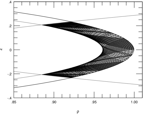
Figure 2: Spheroidal optical resonator as a centrifugal billiard (after 50 reflections)

If all the rays touch the caustic or boundary surface with phases that form stationary distribution (that means that the phase difference along any closed curve on them is equal to integer times $2\pi$), then the eigenfunction and hence eigenfrequency is found.

To find the circular integrals of phases $kS$ (13) we should take into account the properties of phase evolutions on caustic and reflective boundary. Every touching of caustic adds $\pi/2$ (see for example [8]) and reflection adds $\pi$. Thus for $S_{1}$ we have one caustic shift of $\pi/2$ at $\xi_{c}$ and one reflection from the equivalent boundary surface $\xi_{s}$ (at the distance $\sigma$ from the real surface), for $S_{2}$ – two times $\pi/2$ due to caustic shifts at $\pm\eta_{c}$, and we should add nothing for $S_{3}$:

$$k\Delta S_{1}=2k\int\limits_{-\xi_{c}}^{\xi_{s}}\frac{\partial S_{1}}{\partial\xi}d\xi=2\pi(q-1/4)$$

$$k\Delta S_{2}=2k\int\limits_{-\eta_{c}}^{\eta_{c}}\frac{\partial S_{2}}{\partial\eta}d\eta=2\pi(p+1/2)$$

$$k\Delta S_{3}=k\int\limits_{0}^{2\pi}\frac{\partial S_{3}}{\partial\phi}d\phi=2\pi|m|,$$ (15)

where $q=1,2,3...$ – is the order of the mode, showing the number of the zero of the radial function on the surface, and $p=l-|m|=0,1,2...$. These conditions plus integrals (13) completely coincide with those obtained by Bykov [26, 27, 28] if we transform ellipsoidal to spheroidal coordinates, and have clear geometrical interpretation. The integral for $S_{1}$ corresponds to the difference in lengths of the two geodesic curves on $\eta_{c}$ between two points $P_{1}=(\xi_{c},\eta_{c},\phi_{1})$ and $P_{2}=(\xi_{c},\eta_{c},\phi_{2})$. The first one goes from the caustic circle of intersection between $\xi_{c}$ and $\eta_{c}$ along $\eta_{c}$ to the boundary surface $\xi_{s}$, reflects from it, and returns back to the same circle. The second is simply the arc of the circle between $P_{1}$ and $P_{2}$ (Fig.3).

Figure 3: Segments of lines on caustic surfaces determining first quantization rule

The integral for $S_{2}$ corresponds to the length of a geodesic line going from $P_{1}$ along $\xi_{c}$, lowering to $-\eta_{c}$ and returning to $\eta_{c}$ at $P_{2}$ minus the length of the arc of the circle between $P_{1}$ and $P_{2}$.

Figure 4: Segments of lines on caustic surfaces determining second quantization rule

The third integral is simply the length of the circle of intersection of $\xi_{c}$ and $\eta_{c}$.

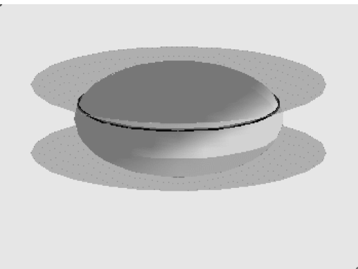
Figure 5: Caustic circle determining third quantization rule

These are elliptic integrals. For the whispering gallery modes when $\eta_{c}\ll 1$ and $\xi_{0}-\xi_{c}\ll\xi_{c}$, $S_{2}$ may be expanded into series over $\eta_{c}$ and $\zeta$ and integrated with the substitutions of $\eta=\eta_{c}\sin\psi$, $\zeta=(\xi^{2}-\xi_{c}^{2})/\xi^{2}_{c}$. Finally, expressing spheroidal coordinates $\xi_{c}$ and expressing $\xi_{0}$ through parameters of spheroid, we have:

$$S_{1} = \frac{nb^{3}}{2a^{2}\sqrt{1+\zeta_{0}}}\int\limits\frac{\sqrt{\zeta}\sqrt{1+\zeta-\eta_{c}^{2}(1+\zeta_{0})(b^{2}-a^{2})/b^{2}}}{(1+\zeta_{0}+(\zeta-\zeta_{0})b^{2}/a^{2})\sqrt{1+\zeta}}d\zeta$$

$$= \frac{nb^{3}}{2a^{2}\sqrt{1+\zeta_{0}}}\left[\frac{2}{3}\zeta^{3/2}-\frac{10a^{2}-4b^{2}}{15a^{2}}\zeta^{5/2}+\frac{a^{2}-b^{2}}{3b^{2}}\zeta^{3/2}\eta^{2}_{c}\right]+O(\zeta^{7/2},\eta_{c}^{2}\zeta^{5/2},\eta_{c}^{4}\zeta^{3/2})$$

$$S_{2} = \frac{nd}{2}\eta^{2}_{c}\int\frac{\cos^{2}\psi\sqrt{\xi_{c}^{2}-s\eta_{c}^{2}\sin^{2}\psi}}{1-\eta_{c}^{2}\sin^{2}\psi}d\psi=\frac{nd}{2}\eta^{2}_{c}\xi_{c}\left[\frac{2\psi+\sin 2\psi}{4}+\frac{(2\xi_{c}^{2}-s)(4\psi-\sin 4\psi)}{64\xi_{c}^{2}}\eta^{2}_{c}\right.$$

$$+ \left.\frac{(8\xi_{c}^{4}-4f\xi_{c}^{2}-1)(12\psi+\sin 6\psi-3\sin 4\psi-3\sin 2\psi)}{1536\xi_{c}^{4}}\eta^{4}_{c}+O(\eta^{6}_{c})\right]$$

$$S_{3} = \mu\phi.$$ (16)

Now we should solve the following system of equations:

$$k\Delta S_{1} = 2kS_{1}(\zeta_{0})\simeq\frac{2\bar{b}^{3}nk\bar{a}}{3\bar{a}^{3}\sqrt{1+\zeta_{0}}}\zeta_{0}^{3/2}\left(1-\frac{5\bar{a}^{2}-2\bar{b}^{2}}{5\bar{a}^{2}}\zeta_{0}-\frac{\bar{b}^{2}-\bar{a}^{2}}{2\bar{b}^{2}}\eta_{c}^{2}\right)=2\pi(q-1/4)$$

$$k\Delta S_{2} = kS_{2}(2\pi)\simeq\pi\frac{nk\bar{b}}{\sqrt{1+\zeta_{0}}}\eta_{c}^{2}\left(1+\frac{\bar{a}^{2}+\bar{b}^{2}}{8\bar{b}^{2}}\eta_{c}^{2}\right)=2\pi(p+1/2)$$

$$k\Delta S_{3} = 2\pi k\mu=2\pi\frac{nk\bar{a}}{\sqrt{1+\zeta_{0}}}\sqrt{1-\frac{\zeta_{0}(\bar{b}^{2}-\bar{a}^{2})}{\bar{a}^{2}}}\sqrt{1-\eta^{2}_{c}}=2\pi|m|,$$ (17)

Using the method of sequential iterations, starting for example from $nk^{(0)}a=l$, $\zeta_{0}^{(0)}=0$, $\eta_{c}^{(0)}=0$ this system may be resolved:

$$\eta_{c}^{2} = \frac{(2p+1)a}{b}l^{-1}\left[1-\frac{\beta_{q}(b^{2}-a^{2})}{2b^{2}}\left(\frac{l}{2}\right)^{-2/3}\right]+O(l^{-2})$$

$$\zeta_{0} = \frac{\beta_{q}a^{2}}{b^{2}}\left(\frac{l}{2}\right)^{-2/3}\left[1+\frac{\beta_{q}(5a^{2}-3b^{2})}{5b^{2}}\left(\frac{l}{2}\right)^{-2/3}\right]+O(l^{-5/3})$$

$$nka = nk(\bar{a}-\sigma_{r})=l+\beta_{q}\left(\frac{l}{2}\right)^{1/3}+\frac{2p(a-b)+a}{2b}-\frac{\chi n}{\sqrt{n^{2}-1}}+\frac{3\beta_{q}^{2}}{20}\left(\frac{l}{2}\right)^{-1/3}$$ (18)

$$+ \frac{\beta_{q}}{12}\left(\frac{2p(a^{3}-b^{3})+a^{3}}{b^{3}}+\frac{2n^{3}\chi(2\chi^{2}-3)}{(n^{2}-1)^{3/2}}\right)\left(\frac{l}{2}\right)^{-2/3}+O(l^{-1}),$$

where for the convenience of comparison we introduced $\beta_{q}=[\frac{3}{2}\pi(q-\frac{1}{4})]^{2/3}$. The value of $\cos\theta$ needed for the calculation of $\Phi_{r}$ (3) one may estimate as $\cos\theta=\sqrt{1-(l+1/2)^{2}/(nk\bar{a})}\simeq\sqrt{\beta_{q}}l^{-1/3}$.

The first three terms for $nka$ were obtained in [3, 26, 27, 28] from different considerations, the last three are new.

To test this series we calculated using finite element method (FEM) eigenfrequencies of TE modes in spheroids with different eccentricities with totally reflecting boundaries for $l=m=100$ (Fig.6). Significant improvement of our series is evident. The divergence of the series for large eccenricities is explained by the fact that the approximation that we used to calculate the integrals (15) but not the method itself breaks down in this case. Namely $\eta_{c}$ becomes comparable to $\xi$ and should not be treated as a small parameter.

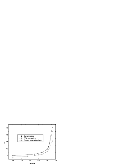
Figure 6: Comparison of the precision of calculation of eigenfrequencies in spheroid for $TE_{100,100,1}$ mode.

If we put $a=b$, then all six terms in the obtained series coincide with that obtained in [9] from exact solution in sphere with a difference that Airy function zeros $\alpha_{q}\simeq(2.3381,4.0879,5.5206,...)$ stand in Schiller’s series instead of approximate $\beta_{q}$ values ($\alpha_{q}-\beta_{q}\simeq$ 0.017; 0.0061; 0.0033, …). The reason is that the eikonal approximation breaks down on caustic, where its more accurate extension with Airy functions is finite [7]. To make our solution even better we may just formally use $\alpha_{q}$ instead of $\beta_{q}$, hence obtaining final formula (1). The eikonal equation for the sphere may be solved explicitly and the expansion of the solution shows that quasiclassical approximation breaks down on a term $O(l^{-1})$, and of the same order should be the error introduced by substitution of vector equations by a scalar ones.

We may now calculate the dependence of mode separation on three indices with up to $O(l^{-2}$ precision:

$$\frac{1}{\omega}\frac{\partial\,\omega}{\partial l}\simeq l^{-1}\left[1-\frac{\alpha_{q}}{6}\left(\frac{l}{2}\right)^{-2/3}\right]$$ (19)

$$\frac{1}{\omega}\frac{\partial\,\omega}{\partial m}\simeq l^{-1}\frac{b-a}{b}\left[1-\frac{\alpha_{q}}{12}\frac{(b-a)(a+2b)}{b^{2}}\left(\frac{l}{2}\right)^{-2/3}\right]$$

$$\frac{1}{\omega}\frac{\partial\,\omega}{\partial q}\simeq\frac{\pi}{2\sqrt{\alpha_{q}}}\left(\frac{l}{2}\right)^{-2/3}\left[1-\frac{\alpha_{q}}{20}\left(\frac{l}{2}\right)^{-2/3}\right]$$

It is interesting to note that when $a=2b$ (oblate spheroid with the eccentricity $\varepsilon=\sqrt{0.75}$, the eigenfrequency separation in the first order of approximation between modes with the same $l$ becomes equal to the separation between modes with different $l$ and the same $l-m$ (free spectral range). The difference appears only in the term proportional to $O(l^{-2/3})$. This situation is close to the case that was experimentally observed in [3]. This new degeneracy has simple quasigeometrical interpretation – like in case of a sphere geodesic lines inclined to the equator plane on such spheroid are closed curves returning at the same point of the equator after the whole revolution, crossing, however, the equator not twice as big circles on a sphere but four times.

4 Arbitrary convex body of revolution

To find eigenfrequencies of whispering gallery modes in arbitrary body of revolution one may use directly the results of the previous section by fitting the shape of the body in convex equatorial area by equivalent spheroid. In fact the body should be convex only in the vicinity of WG mode itself. For example a torus with a width $2R_{T}$ and a height $r_{T}$ may be approximated by a spheroid with $a=R_{T}$ and $b=\sqrt{R_{T}r_{T}}$. Nevertheless, more rigorous approach may be developed.

The first step is to find families of caustic surfaces. This is not a trivial task in general nonintegrable case. The following approximation may be used to find the first family of caustic surfaces [8] which are the place of biinvolute curves for characteristic for a chosen WGM mode geodesic lines on the surface:

$$\sigma_{c}(s) \simeq -\frac{1}{2}\kappa^{2}r_{k}^{1/3}(s)+O(\kappa^{4})$$

$$\cos\theta(s) = \kappa r_{k}^{-1/3}(s),$$ (20)

where $\sigma_{c}(s)$ is the normal distance from a point $s$ on the surface of the body to a caustic surface, $\kappa$ is a parameter of a family, and $r_{k}$ is the radius of curvature of the geodesic line (curvature of the surface in the direction of the beam) and $\cos\theta$ is angle of incidence of the beam in the point $s$.

If we found a caustic surface from the first family, parametrized as $\rho=g(z)$ then we can find also the second family parametrized as $h(z)$ orthogonal to any surface of the first family with different $\kappa$.

A geodesic line for the surface is given by the following integral:

$$\frac{d\phi}{dz}=\frac{\rho_{c}\sqrt{1+g^{\prime 2}}}{g(z)\sqrt{g^{2}(z)-\rho_{c}^{2}}}$$ (21)

where $\rho_{c}=g(z_{m})$ is the radius of caustic circle at maximum distance from equatorial plane. The length of geodesic line:

$$\frac{ds}{dz}=\sqrt{1+g^{\prime 2}+g^{2}\left(\frac{d\phi}{dz}\right)^{2}}=\frac{g\sqrt{1+g^{\prime 2}}}{\sqrt{g^{2}-\rho_{c}^{2}}}$$ (22)

The length of geodesic line, connecting points $\phi_{1}$ and $\phi_{2}$:

$$L^{g}_{1}=2\int\limits_{-z_{m}}^{z_{m}}\frac{g\sqrt{1+g^{\prime 2}}}{\sqrt{g^{2}-\rho_{c}^{2}}}dz$$ (23)

The length of arc from $\phi_{0}=0$ to $\phi_{c}=2\int_{-\eta_{c}}^{\eta_{c}}\frac{d\phi}{du}du$ is equal to $L^{g}_{2}=\rho_{c}\phi_{c}$.

$$L^{g}_{2}=2\int\limits_{-z_{m}}^{z_{m}}\frac{\rho_{c}^{2}\sqrt{1+g^{\prime 2}}}{g\sqrt{g^{2}-\rho_{c}^{2}}}dz$$ (24)

Finally:

$$nk(L^{g}_{1}-L^{g}_{2}) = 2nk\int\limits_{-z_{m}}^{z_{m}}\frac{\sqrt{1+g^{\prime 2}}\sqrt{g^{2}-\rho_{c}^{2}}}{g}dz=2\pi(p+1/2)$$ (25)

In analogous way for another geodesic line on a caustic surface from the other family $\rho=h(z)$ we have

$$nk(L^{h}_{1}-L^{h}_{2}) = 2nk\int\limits_{z_{c}}^{z_{0}}\frac{\sqrt{1+h^{\prime 2}}\sqrt{h^{2}-\rho_{c}^{2}}}{h(z)}dz=2\pi(q-1/4)$$ (26)

The third condition is:

$$2\pi nk\rho_{c}=2\pi|m|$$ (27)

With the substitution $z=\frac{d}{2}\xi_{c}\eta$, $h(z)=\frac{d}{2}\sqrt{\xi_{c}^{2}-s}\sqrt{1-\eta^{2}}$ in (25), and $z=\frac{d}{2}\xi\eta_{c}$, $g(z)=\frac{d}{2}\sqrt{\xi^{2}-s}\sqrt{1-\eta_{c}^{2}}$ in (26) we again obtain expressions for spheroid obtained before (13,15).

5 Quality-factor

As it was shown above, WGMs in axially symmetric bodies, parametrizes as $\rho(z)$ are efficiently described by optical beam traveling close to surface geodesic line and suffering multiple reflections from a curved surface. If we want to calculate Q-factor of whispering gallery mode associated with surface reflection using quasiclassical approach we should take into account losses added at every reflection. The quality factor is determined by the following simple equation [1]:

$$Q=\frac{2\pi n}{\alpha\lambda},$$ (28)

where $\alpha$ denotes losses per unit path length. If the path is comprised of segments of polyline, then the length of each segment is $L_{n}=2r_{k}\cos\theta$, where $r_{k}$ is the radius of curvature of the geodesic line on the surface. Let power losses due to reflection in this segment is equal to $T(\theta)$ and hence $\alpha_{n}=T(\theta,r_{k})/L_{n}$. To account for total losses we should average $\alpha_{n}$ over one coil of geodesic line and hence we finally obtain:

$$Q=\frac{2\pi nL_{g}}{\lambda}\left[\oint\frac{T(\theta)}{2r_{k}(\theta)\cos\theta}dl\right]^{-1}=\frac{2\pi nL_{g}}{\lambda}\left[\int_{-z_{m}}^{z_{m}}\frac{T(\theta)}{r_{k}(\theta)\cos\theta}\frac{dl}{dz}dz\right]^{-1},$$ (29)

This very useful expression can be used to calculate Q-factors in arbitrary shaped whispering gallery resonators associated not only with radiative but also with surface scattering and absorption. The required coefficient $T(\theta)$ may be deduced from the solution of model problem in a sphere, where $r_{k}=a$ and $\cos\theta_{0}=\sqrt{1-(l+1/2)^{2}/(kna)^{2}}\simeq\sqrt{\alpha_{q}}(l/2)^{-1/3}$ are constants:

$$Q_{0}=\frac{4\pi na\cos\theta_{0}}{\lambda T(\theta_{0})},$$ (30)

Radiative losses per single reflection may be also calculated using quasiclassical arguments [29]. If a beam of light is internally reflected from a curved dielectric surface with radius of curvature $r_{k}$, then in the external region evanescent field exponentially decays as $e^{-kr_{n}\sqrt{n^{2}\sin^{2}\theta-1}}$, here $r_{n}$ is normal distance from the surface, however at a distance $r_{n}=r_{k}(n\sin\theta-1)$ tangential phase velocity reaches speed of light and the tail of evanescent field is radiated. These speculations allow to obtain quasiclassical estimate:

$$T = \frac{4n\chi\cos\theta\sqrt{n^{2}\sin^{2}\theta-1}}{n^{2}-1-n^{2}(1-\chi^{2})\cos^{2}\theta}e^{-2\Psi(\theta)},$$

$$\Psi(\theta) = kr_{k}\left[n\sin\theta{\rm arccosh}(n\sin\theta)-\sqrt{n^{2}\sin^{2}\theta-1}\right]$$ (31)

From the above equations one can calculate the Q-factor knowing $T(\theta)$ and using the following expressions:

$$r_{k} = \frac{|{\bf r}^{\prime}|^{3}}{|{\bf r}^{\prime}\times{\bf r}^{\prime\prime}|}=\frac{\rho^{3}(1+\rho^{\prime 2})^{3/2}}{\rho_{m}^{2}(1+\rho^{\prime 2})-\rho\rho^{\prime\prime}(\rho^{2}-\rho_{m}^{2})}$$

$$\frac{dl}{dz} = \frac{\rho(z)\sqrt{1+\rho^{\prime}(z)^{2}}}{\sqrt{\rho^{2}(z)-\rho_{m}^{2}}},$$

$$L_{g} = 4\int_{0}^{z_{m}}\frac{\rho(z)\sqrt{1+\rho^{\prime}(z)^{2}}}{\sqrt{\rho^{2}(z)-\rho_{m}^{2}}}dz,$$

$$\cos(\theta) \simeq \sqrt{2\sigma_{c}/\rho_{k}}$$ (32)

where $\rho_{m}=\rho(z_{m})$ is a distance from the z-axis of the highest point of geodesic line, $\sigma_{c}$ is the normal distance between surface and caustic surface.

For radiative losses, however, only $T(\theta)$ having exponential term essentially variates along the geodesic line with $\cos\theta$ maximal and $\rho_{k}$ minimal at $z=0$ for oblate geometry and vice versa for prolate one.

Now we can calculate the radiative quality factor of WGMs in a spheroid.

$$r_{k} = a\frac{(1+z^{2}(a^{2}-b^{2})/b^{4})^{3/2}}{1+z_{m}^{2}(a^{2}-b^{2})/b^{4}}\simeq a\left(1-\frac{a^{2}-b^{2}}{b^{2}}\eta_{c}^{2}+\frac{3}{2}\frac{a^{2}-b^{2}}{b^{4}}z^{2}\right)$$

$$\sigma_{c} \simeq \zeta_{0}\frac{b^{2}}{2a}\left(1+\frac{a^{2}-b^{2}}{2b^{4}}z^{2}\right)$$

$$\cos\theta \simeq \sqrt{\alpha_{q}}\left(\frac{l}{2}\right)^{-1/3}\left(1+\frac{a^{2}-b^{2}}{2b^{2}}\eta_{c}^{2}-\frac{a^{2}-b^{2}}{2b^{4}}z^{2}\right)$$

$$L_{g} \simeq 2\pi b+\frac{\pi}{2}\frac{a^{2}-b^{2}}{b}\eta_{c}^{2}$$

Using substitution $z=\eta_{c}\cos\psi$ we obtain:

$$Q \simeq \frac{\pi l\sqrt{n^{2}-1}}{4\chi n}\left[\int_{0}^{\pi/2}e^{-2\Psi(\psi)}d\psi\right]^{-1}\simeq\frac{l\sqrt{n^{2}-1}}{2\chi n}e^{2\psi_{0}}\frac{e^{\psi_{1}}}{I_{0}(\psi_{1})}$$

$$\Psi_{0} = nka\left[1-\frac{(2p+1)a(a^{2}-b^{2})}{lb^{3}}\right]\left[{\rm arccosh}(n)\left(1-\frac{\alpha_{q}}{2}\right(\frac{l}{2}\left){}^{-2/3}\right)-\sqrt{1-1/n^{2}}\right]$$

$$\Psi_{1} = \Psi_{0}\frac{3(2p+1)a(a^{2}-b^{2})}{2b^{3}l}$$ (34)

In conclusion. We have analyzed quasiclassical method of calculation of eigenfrequencies and quality factors in dielectrica cavities and found that for spheroid they give rather precise results.

References

- [1] V. B. Braginsky, M. L. Gorodetsky and V. S. Ilchenko, “Quality–factor and nonlinear properties of optical whispering–gallery modes,” Phys. Lett. A137, pp. 393–397, 1989.
- [2] R.D. Richtmyer, “Dielectric Resonators”, J. of Appl. Phys. 10, pp. 391–398, 1939.
- [3] V.S.Ilchenko, M.L.Gorodetsky, X.S.Yao and L.Maleki, “Microtorus: a high–finesse microcavity with whispering–gallery modes”, Opt. Lett. 26, pp. 256–258, 2001.
- [4] K. Vahala, “Optical microcavities”, Nature 424, pp. 839–846, 2001.
- [5] V.S. Ilchenko, A.A. Savchenkov, A.B. Matsko et al. “Nonlinear optics and crystalline whispering gallery mode cavities,” Phys. Rev. Lett. 92, (043903), 2004.
- [6] 2004 Digest of the LEOS Summer Topical Meetings: Biophotonics/Optical Interconnects & VLSI Photonics/WGM Microcavities (IEEE Cat. No.04TH8728), 2004.
- [7] J.B. Keller, S.I. Rubinow, “Asymptotic solution of eigenvalue problems”, Ann. Phys. 9, pp. 24–75, 1960.
- [8] V.M. Babic̆, V.S. Buldyrev, Short-wavelength diffraction theory. Asymptotic methods, Springer-Verlag, Berlin Heidelberg, 1991.
- [9] S.Schiller, “Asymptotic expansion of morphological resonance frequencies in Mie scatternig”, Appl. Opt. ,32, pp. 2181–2185, 1993.
- [10] R. Janaswamy,“A note on the TE/TM decomposition of electromagnetic fields in three dimensional homogeneous space”, IEEE Trans. Antennas and Propagation 52, pp. 2474–2477, 2004.
- [11] S.Asano, G.Yamamoto, “Light scattering by a spheroidal particle”, Appl. Opt. 14, pp. 29–49, 1975.
- [12] V.G. Farafonov, N.V. Voshchinnikov, “Optical properties of spheroidal particles”, Astrophys. and Space Sci. 204, pp. 19–86, 1993.
- [13] A.Charalambopoulos, D.I.Fotiadis, C.V. Massalas, “On the solution of boundary value problems using spheroidal eigenvectors”, Comput. Phys. Comm. 139, pp. 153–171, 2001.
- [14] P.C.G. de Moraes, L.G. Guimarães, “Semiclassical theory to optical resonant modes of a transparent dielectric spheroidal cavity”, Appl. Opt. 41, pp. 2955–2961, 2002.
- [15] L. Li, Z. Li, M. Leong, “Closed-form eigenfrequencies in prolate spheroidal conducting cavity”, IEEE Trans. Microwave Theory Tech. 51, pp. 922–927, 2003.
- [16] I. V. Komarov, L. I. Ponomarev, and S. J. Slavianov, Spheroidal and Coulomb SpheroidalFunctions (in russian) (Moscow: ), Nauka, Moscow, 1976.
- [17] L.Li, X.Kang, M.Leong, Spheroidal Wave Functions in Electromagnetic Theory, John Wiley & Sons, 2002.
- [18] Handbook of Mathematical Functions, ed. M.Abramowitz and I.E.Stegun, National Bureau of Standards, 1964.
- [19] P.C.G. de Moraes, L.G. Guimarães, “Uniform asymptotic formulae for the spheroidal radial function”, J. of Quantitative Spectroscopy and Radiative Transfer 79–80, pp. 973–981, 2003.
- [20] P.C.G. de Moraes, L.G. Guimarães, “Uniform asymptotic formulae for the spheroidal angular function”, J. of Quantitative Spectroscopy and Radiative Transfer 74, pp. 757–765, 2003.
- [21] V.A.Borovikov, B.E.Kinber, Geometrical theory of diffraction, IEE Electromagnet. Waves Ser.37, London, 1994.
- [22] E.L. Silakov,“On the application of ray method for the calculation of complex eigenvalues” (in russian), Zapiski nauchnogo seminara LOMI 42, pp. 228–235, 1974.
- [23] M.Born and E.Wolf, Principles of Optics, 7-th ed., Cambridge University Press, 1999.
- [24] V.I. Arnold, “Modes and quasimodes” (in russian), Funktsionalny analiz i prilozheniya 6, pp. 12–20, 1972.
- [25] M.L.Gorodetsky, V.S.Ilchenko, “High-Q optical whispering-gallery microresonators: precession approach for spherical mode analysis and emission patterns with prism couplers”, Opt. Commun. 113, pp. 133–143, 1994.
- [26] V.P.Bykov, “Geometrical optics of three-dimensional oscillations in open resonators” (in russian), Elektronika bol’schikh moschnostei 4, pp. 66–92, Moscow, 1965.
- [27] L.A. Vainstein,“Barellike open resonators” (in russian), Elektronika bol’schikh moschnostei 3, pp. 176–215, Moscow, 1964.
- [28] L.A. Vainstein, Open Resonators and Open Waveguides, Golem, Denver, 1969.
- [29] G.Roll and G.Scweiger, “Geometrical optics model of Mie resonances”, J.Opt.Soc.Am. A, 17, pp.1301–1311, 2000.
- [30] J.U.Nöckel, “Mode structure and ray dynamics of a parabolic dome microcavity”, Phys. Rev. E, 62, 8677, 2000.
- [31] A.Mekis, J.U.Nöckel, G.Chen, A.D.Stone, and R.K.Chang, “Ray chaos and Q spoiling in Lasing Droplets”, Phys. Rev. Letts, 75, 2682–2685, 1995.