Manifestation of Chaos in Real Complex Systems: Case of Parkinson’s Disease

In this chapter we present a new approach to the study of manifestations of chaos in real complex system. Recently we have achieved the following result. In real complex systems the informational measure of chaotic chatacter (IMC) can serve as a reliable quantitative estimation of the state of a complex system and help to estimate the deviation of this state from its normal condition. As the IMC we suggest the statistical spectrum of the non-Markovity parameter (NMP) and its frequency behavior. Our preliminary studies of real complex systems in cardiology, neurophysiology and seismology have shown that the NMP has diverse frequency dependence. It testifies to the competition between Markovian and non-Markovian, random and regular processes and makes a crossover from one relaxation scenario to the other possible. On this basis we can formulate the new concept in the study of the manifestation of chaoticity. We suggest the statistical theory of discrete non-Markov stochastic processes to calculate the NMP and the quantitative evaluation of the IMC in real complex systems. With the help of the IMC we have found out the evident manifestation of chaosity in a normal (healthy) state of the studied system, its sharp reduction in the period of crises, catastrophes and various human diseases. It means that one can appreciably improve the state of a patient (of any system) by increasing the IMC of the studied live system. The given observation creates a reliable basis for predicting crises and catastrophes, as well as for diagnosing and treating various human diseases, Parkinson’s disease in particular.

1 Introduction

Today the study of manifestations of chaos in real complex systems of diverse nature has acquired great importance. The analysis of some properties and characteristics of real complex systems is impossible without quantitative estimate of various manifestation of chaos. The dynamics or evolution of the system can be predicted by the change of its chaoticity or regularity. The discovery of the phenomenon of chaos in dynamic systems has changed the attitude with regard to the functioning of complex systems, a human organism in particular. The chaos is the absence of regularity. It characterizes the randomness and the unpredictability of the changes of the behavior of a system. At the same time, the presence of chaos in dynamic systems does not mean it cannot be taken under control. Instability of dynamic systems in the state of chaos creates special sensitivity to both external and internal influences and perturbations. The series of weak perturbations of the parameters of the system allows to change its characteristics in the required direction. ”Chaos” is frequently understood as a determined dynamic chaos, that is, the dynamics dependent on the initial conditions, parameters.

Lasers, liquid near to a threshold of turbulence, devices of nonlinear optics, chemical reactions, accelerators of particles, classical multipartite systems, some biological dynamic models are the examples of nonlinear systems with the manifestation of determined chaos. Now manifestations of chaos are being studied in different spheres of human activity.

The control of the behavior of chaotic systems is one of the most important problems. Most of the authors see two basic approaches to solve the problems Boc ; Touc . Both directions envisage a preliminary choice of a certain perturbation. The selected perturbation is used to exert influence on the chaotic system. The first direction relies on an internal perturbation, the choice of which is based on the state of the system. The perturbation changes the parameter or the set of parameters of the system, which results in the ordered behaviour of the chaotic systems. The methods focusing on the choice of such parameters (perturbations) are referred to as ”methods with a feedback” Boc -Plapp . They do not dependent on the studied chaotic system (model) as these parameters can be selected by observing the system for some period of time. One also considers that the methods with a delayed feedback Pyr ; Just belong to the first direction. The second approach presupposes that the choice of the external perturbation does not dependent on the state of the chaotic system under consideration. By affecting the studied system with the similar perturbation, it is possible to change its behaviour. The present group of methods is an alternative to the first one. These methods can be used in cases when internal parameters depend on the environment Boc ; Lima ; Braim .

Generally, when choosing internal (external) perturbations it is possible to determine three basic stapes: the estimation of the initial information, the choice of the perturbation and the bringing the chosen strategy of control into action (its practical realization). At the first stage the information on the state of the studied system is collected. At the second stage the received information is processed according to the plan or strategy of the control. On the basis of the achieved results the decision on the choice of the internal (of the external) perturbation is accepted. After that the chosen strategy of chaos control is put into practice Touc .

The initial idea of the present concept was to separate Markov (with short-range time memory) and non-Markov (with long-range time memory) stochastic processes. However, the study of real complex systems has revealed additional possibilities of the given parameter. Actually, the non-Markovity parameter represents a quantitative measure of chaoticity or regularity of various states of the studied system. An increase of the given parameter ($\varepsilon_{1}(0)\gg 1$) corresponds to an increase of the chaoticity of the state of the system. A decrease of the non-Markovity parameter means a greater ordering (regularity) of the state of the system. The given observation allows one to define a new strategy for estimating of chaoticity in real systems. This new approach in chaos theory can be presented as an alternative to the existing methods. Further analysis of the non-Markovity parameter allows one to define the degree of chaoticity or regularity of a state of the system.

In this work the new strategy for the study of manifestations of chaoticity is applied to real complex systems. The possibilities of the new approach are revealed at the analysis of the experimental data on various states of a human organism with Parkinson’s disease. Parkinson’s disease is a chronic progressing disease of the brain observed in 1-2 % of elderly people. The given disease was described in 1817 by James Parkinson in the book ”An essay on the shaking palsy”. In 19th century the French neurologist Pierre Marie Charcot called this disease ”Parkinson’s disease”. The steady progress of the symptoms and yearly impairment of motor function is typical of Parkinson’s disease. Complex biochemical processes characteristic of Parkinson’s disease result in a lack of dopamine, a chemical substance which is carrier signals from one nerve cell to another. The basic symptoms typical of Parkinson’s disease form the so-called classical triad: tremor, rigidity of muscles (disorder of speech, amimia), and depression (anxiety, irritability, apathy). The disease steadily progresses and eventually the patient becomes a helpless invalid. The existing therapy comprises a set of three basic treatments: medical treatment, surgical treatment and electromagnetic stimulation of the affected area of the brain with the help of an electromagnetic stimulator. Today this disease is considered practically incurable. The treatment of patients with Parkinson’s disease requires an exact estimate of the current state of the person. The offered concept of research of manifestations of chaoticity allows one to track down the least changes in the patient with the help of an exact quantitative level of description.

Earlier we found out an opportunity for defining the predisposition of a person to the frustration of the central nervous system due to Parkinson’s disease Yulm4 . Our work is an expansion and development of the informational possibilities of the statistical theory of discrete non-Markov random processes and the search for parameters affecting the health of a subject.

2 The statistical theory of discrete non-Markov random processes. Non-Markovity parameter and its frequency spectrum

The statistical theory of discrete non-Markov random processes Yulm1 -Yulm3 forms a mathematical basis for our study of complex live systems. The theory allows one to calculate the wide quantitative set of dynamic variables, correlation functions and memory functions, power spectra, statistical non-Markovity parameter, kinetic and relaxation parameters. The full interconnected set of these variables, functions and parameters creates a quantitative measure of chaoticity used for the description of processes, connected with functioning of alive organism.

We use the non-Markovity parameter $\varepsilon$ as a quantitative estimate of the non-Markov properties of the statistical system. The non-Markovity parameter allows to statistical processes into Markov processes ($\varepsilon\rightarrow\infty$), quasi-Markov processes ($\varepsilon>1$) and non-Markov processes ($\varepsilon\sim$1). Besides the non-Markovity parameter we also use the spectrum of the non-Markovity parameter. We define the spectrum as the set of all values of the physical parameter used for describing the state of a system or a process. Let’s consider the first and the $n$th kinetic equations of the chain of connected non-Markov finite-difference kinetic equations Yulm1 ; Yulm2 :

$$\frac{\Delta a(t)}{\Delta t}=\lambda_{1}a(t)-\tau\Lambda_{1}\sum_{j=0}^{m-1}M_{1}(j\tau)a(t-j\tau),$$ (1)

$$\cdots$$

$$\frac{\Delta M_{n}(t)}{\Delta t}=\lambda_{n+1}M_{n}(t)-\tau\Lambda_{n+1}\sum_{j=0}^{m-1}M_{n+1}(j\tau)M_{n}(t-j\tau).$$

The first equation is based on the Zwanzig’-Mori’s kinetic equation in nonequilibrium statistical physics:

$$\frac{da(t)}{dt}=-\Omega^{2}_{1}\int_{0}^{t}d\tau M_{1}(j\tau)a(t-j\tau).$$

Here $a(t)$ is a normalized time correlation function (TCF):

$$\lim_{t\to 0}a(t)=1,\lim_{t\to\infty}a(t)=0.$$

The zero memory function $a(t)$ and the first order memory function $M_{1}(t)$ in (1):

$$M_{0}(t)=a(t)=\frac{<{\bf A}_{k}^{0}(0){\bf A}_{m+k}^{m}(t)>}{<|{\bf A}_{k}^{0}(0)|^{2}>},~{}~{}t=m\tau,$$

$$M_{1}(j\tau)=\frac{<{\bf A}_{k}^{0}(0)\hat{L}_{12}\{1+i\tau\hat{L}_{22}\}^{j}\hat{L}_{21}{\bf A}_{k}^{0}(0)>}{<{\bf A}_{k}^{0}(0)\hat{L}_{12}\hat{L}_{21}{\bf A}_{k}^{0}(0)>},~{}~{}M_{1}(0)=1.$$

$${\bf A}_{k}^{0}(0)=(\delta x_{0},\delta x_{1},\delta x_{2},\cdots,\delta x_{k-1}),$$

$${\bf A}_{m+k}^{m}(t)=\{\delta x_{m},\delta x_{m+1},\delta x_{m+2},\cdots,\delta x_{m+k-1}\},$$

describes statistical memory in complex systems with a discrete time (${\bf A}_{k}^{0}(0)$ and ${\bf A}_{m+k}^{m}(t)$ are the vectors of the initial and final states of the studied system). The operator $\hat{L}$ is a finite-difference operator:

$$i\hat{L}=\frac{\bigtriangleup}{\bigtriangleup t},\ \ \bigtriangleup t=\tau,$$

where $\tau$ is a discretization time step, $\hat{L}_{ij}=\Pi_{i}\hat{L}\Pi_{j}$ ($i,j=1,2$) are matrix elements of the splittable Liouville’s quasioperator, $\Pi_{1}=\Pi,\Pi_{2}=P=1-\Pi$ and $\Pi$ are projection operators.

Let’s define the relaxation times of the initial TCF and of the first-order memory functions as follows $M_{1}(t)$:

$$\tau_{a}=Re\int_{0}^{\infty}a(t)dt,\tau_{M_{1}}=Re\int_{0}^{\infty}M_{1}(t)dt,\cdots,\tau_{M_{n}}=Re\int_{0}^{\infty}M_{n}(t)dt.$$

Then the spectrum of the non-Markovity parameter $\{\varepsilon\}$ is defined as an infinite set of dimensionless numbers:

$$\{\varepsilon_{i}\}=\{\varepsilon_{1},\varepsilon_{2},...,\varepsilon_{n},...\},$$

$$\varepsilon_{1}=\tau_{a}/\tau_{M_{1}},\varepsilon_{2}=\tau_{M_{1}}/\tau_{M_{2}},\cdots,\varepsilon_{n}=\tau_{M_{n}}/\tau_{M_{n+1}},$$

$$\varepsilon=\tau_{rel}/\tau_{mem}.$$ (2)

Note that $a(t)=M_{0}(t).$ The number $\varepsilon_{n}$ characterizes the ratio of the relaxation times of the memory functions $M_{n}$ and $M_{n+1}$. If for some $n$ the value of the parameter $\varepsilon_{n}\to\infty$, then this relaxation level is Markovian. If $\varepsilon_{n}$ changes in limits from zero to a unit value, then the relaxation level is defined as non-Markovian. The times $\tau_{rel}$ (relaxation time) and $\tau_{mem}$ (memory life time) appear when the effects of the statistical memory in the complex discrete system are taken into account by means of the Zwanzig’-Mori’s method of kinetic equations. Thus, the non-Markovity parameter spectrum is defined by the stochastic properties of the TCF.

In Yulm1 the concept of generalized non-Markovity parameter for a frequency - dependent case was introduced:

$$\varepsilon_{i}(\omega)=\left\{\frac{\mu_{i-1}(\omega)}{\mu_{i}(\omega)}\right\}^{\frac{1}{2}}.$$ (3)

Here as $\mu_{i}(\omega)$ we have the frequency power spectrum of the i$th$ memory functions: $\mu_{1}(\omega)=|Re\int_{0}^{\infty}M_{1}(t)e^{i\omega t}dt|^{2},\cdots,\mu_{i}(\omega)=|Re\int_{0}^{\infty}M_{i}(t)\\ e^{i\omega t}dt|^{2}.$

The use of $\varepsilon_{i}(\omega)$ allows one to find the details of the frequency behaviour of the power spectra of the time correlations and memory functions.

3 The universal property of informational manifestation of chaoticity in complex systems

In our work the discussion of manifestation of chaoticity is carried out on the basis of a statistical invariant which includes a quantitative informational measure of chaoticity and pathology in a covariant form. The existence of this invariant is very important for the taking decisions in the problems related to medicine as well as for analysing a wide area of physical problems related to complex systems of various nature.

In each live organism there is a universal informational property of the following form:

$$IMC+IMP=Invariant.$$ (4)

Here IMC is an informational (quantitative) measure of chaoticity for the concrete live system, IMP is an informational measure of a pathological state of a live organism. As an informational (quantitative) measure of the degree of chaoticity (regularity) we propose to use the first point of the non-Markovity parameter at zero frequency: $\varepsilon_{1}(0)=\left\{\frac{\mu_{0}(0)}{\mu_{1}(0)}\right\}^{\frac{1}{2}}$. The physical sense of the parameter consists in comparison the relaxation scales of the time correlation function ($a(\omega)$) to the memory functions of the first order ($\mu(\omega)$). Depending on the values of this parameter one can discriminate Markov processes (with short-range memory) and non-Markov processes (with effects long-range memory). Thus, the phenomena distinguished by the greatest chaoticity correspond to Markov processes. Non-Markov processes are connected with greater regularity. The informational measure of a pathological state (IMP) defines the qualitative state of a real live system.

The quantitative estimate IMC of the degree of the chaoticity of system contains the information on a pathological state of the system. It testifies to the close interrelation of the given quantities. A high degree of chaoticity is characteristic of a normal physiological state. In a pathological state the degree of chaoticity decreases. A high degree of regularity is typical of this condition. Thus, the quantitative estimate of chaoticity in live systems allows one to define their physiological or pathological state with a high degree of accuracy. In the right-hand side of (4) we have a statistical invariant, which reveals the independence of the physical (as well as biophysical, biochemical and biological) laws in the given live organism from the concrete situations as well as the methods of description of these situations. The invariance, submitted in (4), is formulated as the generalization of the experimental data. Among other physical laws the properties of invariance reflect the most general and profound properties of the studied systems and characterize a wide sphere of phenomena. Equation (4) reflects an informational observation. It consists of two informational measures: the measure of chaoticity and the measure of pathology (disease).

Let’s use the operator of transformation $T(S^{\prime},S)$ in both parts of (4). It realizes the transition of the system from one state $S$ to other $S^{\prime}$. By taking into account the statistical invariance $I(S^{\prime})=T(S^{\prime},S)I(S)=I(S)$ in the right-hand side of (4) we get:

$$\Delta P=P(S^{\prime})-P(S)=-\Delta C=-\{C(S^{\prime})-C(S)\},\Delta P+\Delta C=0.$$ (5)

Here the following designations are introduced: $I(S)$ = $Invariant$, $P(S)=IMP(S)$ is an informational measure of pathology (disease) for the state $S$, $C(S)=IMC(S)$ is an informational measure of chaoticity for the state of patient $S$. Besides in (5) we take into account the rules of transformation:

$$C(S^{\prime})=T(S^{\prime},S)C(S),P(S^{\prime})=T(S^{\prime},S)P(S).$$ (6)

Equations (4)-(6) are rather simple but they make the quantitative description of the state of a patient possible, both during the disease and under the medical treatment. Equations (4)-(6) have a general character. They are true for many complex natural and social systems. It is possible to develop the algorithms of prediction of various demonstrations of chaos in complex systems of diverse nature on the basis of these equations.

4 The quantitative factor of quality of a treatment

One of the major problems of the medical physics consists in the development of a reliable criterion to estimate the quality of a medical treatment, a diagnosis and a forecasting of the behaviour of real live complex systems. As one can see from the previous section, such a criterion should include the parameter of the degree of randomness in a live organism. The creation of a quantitative factor for the quality of a treatment $Q_{T}$ is based on the behaviour law of the non-Markovity parameter $\varepsilon_{1}(0)$ in the stochastic dynamics of complex systems. The greater values of the parameter $\varepsilon_{1}(0)$ are characteristic of stable physiological states of systems; the smaller ones are peculiar for pathological states of live systems. Thus, by the increase or reduction of the non-Markovity parameter one can judge the physiological state of a live organism with a high degree of accuracy. Therefore the non-Markovity parameter allows one to define the deviation of the physiological state of a system from a normal state.

The factor $Q_{T}$ defines the efficacy or the quality of the treatment and is directly connected with the changes in the quantitative measure of chaoticity in a live organism. We shall calculate it in a concrete example. Let us consider 1 as the patient’s state before therapy, and 2 as the state of the patient after certain medical intervention. Then $\varepsilon_{1}(\textbf{1})$ and $\varepsilon_{1}(\textbf{2})$ represent quantitative measures of the chaoticity for the physiological states 1 and 2. The ratio $\delta$ of these values ($\delta=\frac{\varepsilon_{1}(\textbf{2})}{\varepsilon_{1}(\textbf{1})}$) will define efficacy of the therapy. Various $j$th processes occur simultaneously in the therapy. Therefore the total value of $\delta$ can be defined by the following way:

$$\delta=\prod_{j=1}^{n}\frac{\varepsilon_{1}^{j}(\textbf{2})}{\varepsilon_{1}^{j}(\textbf{1})},$$ (7)

where $j=1,2...n$ is the number of factors affecting the behaviour of the non-Markovity parameter. However, the natural logarithm $\ln\delta$ is more convenient for use.

Then we have:

$$\delta>1,\ln\delta>0;$$

$$\delta=1,\ln\delta=0;$$

$$\delta<1,\ln\delta<0.$$

The three values of $\delta$ mentioned above correspond to the three different situations of treatment: effective, inefficient and destructive treatment. They reflect an increase, preservation and reduction of the measure of the chaoticity in the therapy. Thus, one can define $Q_{T}(\varepsilon)=\ln\delta$ according to (7) as follows:

$$Q_{T}{(\varepsilon)}=\ln\prod_{j=1}^{n}\frac{\varepsilon_{1}^{j}(\textbf{2})}{\varepsilon_{1}^{j}(\textbf{1})}.$$ (8)

However, the total factor $Q_{T}$ is defined both by the quantitative measures of the chaoticity and by other physiological and biochemical data. Now we shall consider the transition of the patient from state 1 into state 2. Then by analogy, one can introduce the physiological parameter $k(\textbf{1})$, determined for state 1, and $k(\textbf{2})$ for state 2. In the case of Parkinson’s disease one can introduce the amplitude or the dispersion of the tremor velocity of some extremities (hand or leg) of the patient as this parameter. In other cases any medical data, which is considered for diagnostic purposes, can be used. For greater reliability it is necessary to use the combination of various parameters $k^{j}(\textbf{1})$ and ($k^{j}(\textbf{2})$).

The value:

$$Q_{T}=\ln\prod_{j=1}^{n}\frac{\varepsilon_{1}^{j}(\textbf{2})}{\varepsilon_{1}^{j}(\textbf{1})}*\left\{\frac{k^{j}(\textbf{2})}{k^{j}(\textbf{1})}\right\}$$ (9)

will be considered as a generalized quantitative factor of quality of the therapy.

However in real conditions it is necessary to increase or weaken the magnitude of chaotic, or physiological contributions to (9). For this purpose we shall take the simple ratio:

$$\ln\prod(a^{n}b^{m}...)=n\ln a+m\ln b+...$$

By analogy, we can reinforce or weaken various contributions depending on the concrete situation:

$$Q_{T}=\ln\prod_{j=1}^{n}\left(\frac{\varepsilon_{1}^{j}(\textbf{2})}{\varepsilon_{1}^{j}(\textbf{1})}\right)^{m_{j}}*\left\{\frac{k^{j}(\textbf{2})}{k^{j}(\textbf{1})}\right\}^{p_{j}}.$$ (10)

If incomplete experimental data are available in some situations, one can assume $p_{j}=1$ (attenuation of the physiological contribution). A value of $m_{j}>1$ can mean an amplification of the chaotic contribution. Otherwise, if we want to weaken the chaotic contribution, we should take ($m_{j}=1$) and if we want to reinforce the physiological contribution we come towards ($p_{j}>1$). We have presented the results of the calculation of the quantitative factor $Q_{T}$ below in Sect. 6.

5 Experimental data

We have taken the experimental data from Beuter1 . They represent the time records of the tremor velocity of the index finger of a patients with Parkinson’s disease (see, also http://physionet.org/physiobank/database/). The effect of chronic high frequency deep brain stimulation (DBS) on the rest tremor was investigated Beuter1 in a group of subjects with Parkinson’s disease (PD) (16 subjects). Eight PD subjects with high amplitude tremor and eight PD subjects with low amplitude tremor were examined by a clinical neurologist and tested with a velocity laser to quantify time and frequency domain characteristics of tremor. The participants received DBS of the internal globus pallidus (GPi), the subthalamic nucleus (STN) or the ventrointermediate nucleus of the thalamus (Vim). Tremor was recorded with a velocity laser under two conditions of DBS (on-off) and two conditions of medication (L-Dopa on-off).

All the subjects gave informed consent and institutional ethics procedures were followed. The selected subjects were asked to refrain from taking their medication at least 12 h before the beginning of the tests and were not allowed to have more than one coffee at breakfast on the two testing days. Rest tremor was recorded on the most affected side with a velocity-transducing laser Beuter2 ; Norm . This laser is a safe helium-neon laser. The laser was placed at about 30 cm from the index finger tip and the laser beam was directed perpendicular to a piece of reflective tape placed on the finger tip. Positive velocity was recorded when the subjects extended the finger and negative velocity when the subjects flexed the finger.

The conditions, counterbalanced across subjects, included the following:

1. The L-Dopa condition (no stimulation).

2. The DBS condition (stimulation only).

3. The ”off” condition (no medication and no stimulation).

4. The ”on” condition (on medication and on stimulation).

5. The effect of stopping DBS on tremor (time record of the tremor after 15, 30, 45, 60 min since switching off of the stimulator).

In Fig. 1 the time records of the velocity of changing tremor of the index finger of the second patient’s hand (man, 52 years old) under various conditions of influence on the organism are submitted as an example. High velocity of tremor is observed: 1) in a natural condition of the patient (a), 2) 15 (45) minutes after the stimulator was switched off. Lower tremor speed occurs: 1) when both methods (stimulation, medication) are used, 2) when each of these methods is used separately, 3) 30 (60) minutes after the stimulator was switched off. Similar results are presented in Beuter1 .

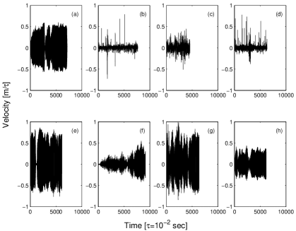
Figure 1: The velocity of the change of tremor of the right index finger of the patient’s right hand (the second subject) with Parkinson’s disease under various conditions of the experiment. (a) deep brain stimulation off, medication off; (b) the subject was receiving stimulation of the GPi, medication on; (c) deep brain stimulation off, medication on; (d) the subject was receiving stimulation of the GPi, medication off; (e)-(h) the recording of rest tremor in the right index finger of the subject 15 (30, 45, 60) minutes after the stimulator was switched off, this subject was off medication for at least 12 hours

6 Results

In this section the results obtained by processing the experimental data for one of the patients (subject number 2) are shown. Similar or related pictures are observed in the experimental data of other subjects.

6.1 The non-Markovity parameter as a quantitative measure of defining chaoticity

In this subsection the technique to calculate quantitative and qualitative criteria under various conditions influencing the state of a patient is given. The basic idea of the approach consists in defining the quantitative ratio between chaoticity and regularity of the observed process. It allows one to judge the physiological (pathological) state of a live system by the degree of chaoticity or of regularity. The highest degree of chaoticity in the behaviour of a live system corresponds to a normal physiological state. Higher degree of regularity or specific ordering is characteristic of various pathological states of a live system. In the given work we use the non-Markovity parameter $\varepsilon_{1}(0)$ as a special quantitative measure defining chaoticity or regularity of the studied process. The examples Yulm1 -Yulm5 , Yulm6 which have been investigated by us earlier serve as a basis for such reasoning. As one of the examples we shall consider the tremor velocity of the changing of the subject’s index fingers in the case of Parkinson’s disease.

The comparative analysis of the initial time record and the non-Markovity parameter for all the submitted experimental data allows one to discover the following regularity. The value of the non-Markovity parameter $\varepsilon_{1}(0)$ decreases with the increase of the tremor velocity of the patient’s fingers (deterioration of the physiological state) and grows with the decrease of the tremor velocity (improvement of the state of the patient). We shall also consider the power spectra $\mu_{0}(\omega)$ of the initial TCF under various conditions influencing an organism, the window-time behaviour of the power spectrum $\mu_{0}(\omega)$ and the non-Markovity parameter $\varepsilon_{1}(\omega)$, the time dependence local averaging relaxation parameter $\lambda_{1}(t)$ as additional sources of information.

Figure 2 represents the power spectra of the initial TCF for various experimental conditions. One can observe the powerful peak in all the figures at the characteristic frequency $\omega=0.07f.u.(\omega=2\pi\nu,1f.u.=2\pi/\tau,1\tau=10^{-2}$ second). The amplitude values of this peak for $\mu_{i}(\omega)$ ($i=1,2,3$) are given in Table 1. The given peak testifies to a pathological state of the studied system. A similar picture is observed in patients with myocardial infarction Yulm2 . The comparison of these values reflects the amplitude of the tremor velocity at the initial record of time.

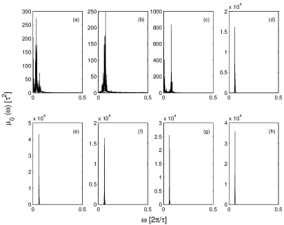
Figure 2: The power spectrum $\mu_{0}(\omega)$ of the initial TCF for the velocity of changing of tremor of subject number 2 under various conditions that influence an organism. (a) deep brain stimulation on, medication on; (b) deep brain stimulation on, medication off; (c) deep brain stimulation off, medication on; (d) deep brain stimulation off, medication off; (e)-(h) the power spectrum $\mu_{0}(\omega)$ of the initial TCF for the recording of rest tremor in the right index finger of the subject 15 (30, 45, 60) minutes after the stimulator was switched off, medication off. At the frequency $\omega=0.07f.u.,1f.u.=100Hz$ (the characteristic frequency), a peak is found. The presence and amplitude of this peak are determined by the state of the patient

Table 1. The value $\mu_{0}(\omega)$ for the initial TCF and $\mu_{i}(\omega)$ ($i=1,2,3$) for the memory functions of junior orders at the frequency $\omega=0.07f.u.$ 1 - Deep brain stimulation, 2 - Medication (subject number 2). For example, OFF OFF - no DBS and no medication. ON ON ON OFF OFF ON OFF OFF 15 OFF 30 OFF 45 OFF 60 OFF $\mu_{0}$ 75 250 812 $1.71*10^{4}$ $4.34*10^{4}$ $1.53*10^{4}$ $2.51*10^{4}$ $3.68*10^{4}$ $\mu_{1}$ 19 52 $1.28*10^{3}$ $1.17*10^{4}$ $3.21*10^{4}$ $1.32*10^{4}$ $1.82*10^{4}$ $2.8*10^{4}$ $\mu_{2}$ 42 60 113 71 300 62 137 224 $\mu_{3}$ 37 54 141 73 147 74 152 186

In Table 1 the second patient’s amplitude values $\mu_{0}(\omega)$ for the initial TCF and the memory functions of junior orders $\mu_{i}(\omega)$ ($i=1,2,3$) at the frequency $\omega=0.07f.u.$ are submitted. The terms of the first row define the conditions under which the experiment is carried out. Under all conditions a power peak at the frequency $\omega=0.07f.u.$ can be observed. The amplitude values of the given peak (in particular in the power spectrum $\mu_{0}(\omega)$) reflect the amplitude of the tremor velocity. For example, the least amplitude 75 $\tau^{2}$ corresponds to the condition (ON, ON; or: deep brain stimulation on, medication on). The highest amplitude $4.34*10^{4}\tau^{2}$ corresponds to the greatest tremor speed (see Figs. 1e, 2e). Thus, the given parameter can be used to estimate the physiological state of a patient. A similar picture is observed in all other patients.

In Fig. 3 the initial time record (the normal state of the subject; OFF, OFF) and the window-time behaviour of the power spectrum of the TCF (the technique of the analysis of the given behaviour is considered in Ref. Yulm6 ) are submitted. In these figures regions 1, 2, 3, which correspond to the least values of the tremor velocity are shown. The minimal amplitude of the peaks of the power spectrum $\mu_{0}(\omega)$ corresponds to the regions with the least tremor velocity.

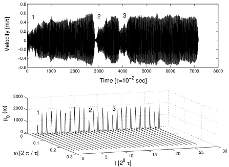
Figure 3: The initial time series and the window-time behaviour of the power spectrum $\mu_{0}(\omega)$ of the TCF. Two figures are submitted to illustrate the case of subject number 2: no stimulation of the brain and no medication. The change of regimes in the initial time series is reflected in the decrease of the tremor velocity (regions 1, 2 and 3) and becomes visible as a sharp reduction of the power of spectrum $\mu_{0}(\omega)$ (see, the $1th,12th,17th$ windows for more detail)

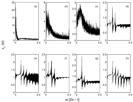
Figure 4: The first point of the non-Markovity parameter $\varepsilon_{1}(\omega)$ for the second subject under various experimental conditions: (a) deep brain stimulation off, medication on; (b) deep brain stimulation on, medication on; (c) deep brain stimulation on, medication off; (d) deep brain stimulation off, medication off; (e)-(h) the recording of rest tremor in the right index finger of the subject 15 (30, 45, 60) minutes after the stimulator was switched off, medication off. The non-Markovity parameter at zero frequency $\varepsilon_{1}(0)$ plays a special role. These values (6.02 in the first case and 1.0043 in the last one) define chaoticity or the regularity of the studied states. The amplitudes of these values also characterize the state of the subject

In Fig. 4 the frequency dependence of the first point of the non-Markovity parameter $\varepsilon_{1}(\omega)$ is submitted for the second subject under various experimental conditions. The value of the parameter $\varepsilon_{1}(0)$ at zero frequency is of special importance for our study of manifestations of chaoticity. It is possible to judge the change of the state of a subject by the increase (or by the decrease) of this value. The comparative analysis of the initial time records allows one to come to the similar conclusions. In Figs. 4d-h a well-defined frequency structure of the non-Markovity parameter can be seen. The structure is completely suppressed and disappears only when during the treatment. The characteristic frequency of the fluctuations corresponds approximately to $\omega=0.06f.u.$ These multiple peaks are the most appreciable at low frequencies. At higher frequencies these fluctuations are smoothed out. As can be seen in these figures, the 2nd subject has a strong peak which remains stable over time. As our data show, the comb-like structure with multiple frequencies can be observed in all patients with high tremor velocity. In a group of patients with low tremor velocity it disappears, and a wider spectrum that presents some fluctuations over time is observed. The present structure testifies to the presence of characteristic frequency of fluctuations of tremor of human extremities.

In Table 2 the dispersion interval of the values and the average value $\varepsilon_{1}(0)$ for the whole group of subjects (16 subjects) are submitted. Let us consider 2 conditions: OFF, OFF and OFF, ON. In the first case the dispersion interval and the average value $\varepsilon_{1}(0)$ are minimal. It means the presence of a high degree of regularity of the physiological state of the patient. The degree of regularity is appreciably reduced when applying any method of treatment. Here the degree of chaoticity grows. The maximal degree of chaoticity corresponds to the condition OFF, ON (medication is used only). The difference in $\varepsilon_{1}(0)_{av.val}$ with medication and without it (OFF, OFF) is 3.8 times (!). On the basis of the comparative analysis of the given parameters the best method of treatment for each individual case can be found. It is necessary to note, that the given reasoning is true only for the study of the chaotic component of the quantitative factor of the quality of treatment $Q_{T}$. The most trustworthy information about the quality of treatment can be given by the full quantitative factor $Q_{T}$ which takes into account of other diagnostic factors.

Table 2. The dispersion interval $\varepsilon_{1}(0)_{int}$ of the values and the average value $\varepsilon_{1}(0)_{av.val}$ of the first point of the non-Markovity parameter under various experimental conditions for the group of 16 subjects. 1 - Deep brain stimulation, 2 - Medication.

	OFF OFF	ON OFF	OFF ON	ON ON	15 OFF	30 OFF	45 OFF	60 OFF
$\varepsilon_{1}(0)_{int}$	1 - 1.8	2 - 18	2 - 22	1.5 - 8	1.5 - 3	1.8 - 5	1.7 - 4.5	2 - 6
$\varepsilon_{1}(0)_{av.val}$	1.41	4.14	5.31	3.17	2.43	2.92	2.76	2.93

The results of the calculation of the quantitative factor $Q_{T}$ are shown in Table 3. The data are submitted for a single patient and for the whole group. Here $Q_{T}(\varepsilon)$ is the chaotic contribution to the quantitative factor (see (8)). $Q_{T}$ is the total quantitative factor (see (10)), where $\varepsilon^{(1)}(\textbf{1})$ and $\varepsilon^{(1)}(\textbf{2})$ are the chaotic contributions for the tremor amplitudes $k^{(1)}(\textbf{1}),k^{(1)}(\textbf{2})$; $\varepsilon^{(2)}(\textbf{1})$ and $\varepsilon^{(2)}(\textbf{2})$ are the dispersions of the tremor amplitudes $k^{(2)}(\textbf{1}),k^{(2)}(\textbf{2})$ (physiological contributions). The full factor $Q_{T}$ provides detailed information about the quality of the treatment. The present factor includes both the chaotic component $Q_{T}(\varepsilon)$, and the physiological contribution $Q_{T}(k)$. The calculation $Q_{T}(k)$ is described in Sect. 4. One can define the quality of a treatment by means of $Q_{T}$. The positive value of the given factor defines an effective treatment. For a separate patient and for the whole group, $Q_{T}$ reaches its maximal value under the condition ON, ON. The total quantitative factor is supplemented by a diagnostic (physiological) component. It allows one to take into account those features of the system which the chaotic component does not contain. For the second patient under condition 15 OFF (see Table 3) the factor $Q_{T}$ has a negative value. It testifies to the negative influence of the given treatment on the organism of the patient. The best treatment is thus the combination of the two medical methods: electromagnetic stimulation and medication.

Table 3. The quantitative factor $Q_{T}(\varepsilon)$ and the total quantitative factor $Q_{T}$ for the second patient and for the whole group (16 subjects). 1 - Deep brain stimulation, 2 - Medication. $m_{j}=1,p_{j}=1.$

				The 2 patient
	OFF OFF	ON OFF	OFF ON	ON ON	15 OFF	30 OFF	45 OFF	60 OFF
$Q_{T}(\varepsilon)$		0.758	2.556	1.756	0.291	0.438	0.041	0.017
$Q_{T}$		1.763	2.013	2.654	-0.013	0.883	-0.004	0.856
				The all group
$Q_{T}(\varepsilon)$		1.077	1.326	0.810	0.544	0.728	0.671	0.731
$Q_{T}$		3.661	2.883	4.071	1.47	1. 734	1.624	1.742

Figure 5 reflects the behaviour of the parameter $\varepsilon_{1}(0)$ for four different patients. The points lying above the horizontal line testify to an improvement of the state of the subject and the efficacy of the treatment. The points, lying below the horizontal line testify to a deterioration of the state of the subject and the inefficiency of the applied method. For example, Fig. 5b corresponds to the sevenfold change of the quantitative measure of chaoticity for the 9th patient. In case of the 8th patient (see Fig. 5c) no influence could change the measure of the chaoticity. Therefore there was practically no change in the state of the subject either. In some cases (see Figs. 5b, 5d) the DBS or the medication reduces the measure of chaoticity which testifies to a deterioration of the state of the subject. This approach allows one to define the most effective (or inefficient) treatment in each individual case.

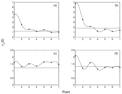
Figure 5: The behavior of the parameter $\varepsilon_{1}(0)$ for four various patients: (a) the second subject, high amplitude tremor, (b) the 9th subject, low amplitude tremor (the stimulation of the GPi); (c) the 8th subject, high amplitude tremor, (d) the 15th subject, low amplitude tremor (the stimulation of the STN). The value of $\varepsilon_{1}(0)$ for seven consecutive conditions of the experiment: 1 - both methods are used; 2 - treatment by medication is applied only; 3 - the DBS is used only; 4 (5, 6, 7) - value of the parameter 15 (30, 45, 60) minutes after the stimulator was switched off; the horizontal line corresponds to the value of the parameter when no method is used. This representation allows one to define the most effective treatment for each patient

6.2 The definition of a predictor of sudden changes of the tremor velocity

In this subsection the window-time behaviour of the non-Markovity parameter $\varepsilon_{1}(\omega)$ for a certain case (the second patient, two methods of medical treatment were used) and the procedure of local averaging of the relaxation parameters are considered. These procedures allow one to determine specific predictors of the change of regimes in the initial time records.

The idea of the first procedure is, that the optimum length of the time window ($2^{8}=256$ points) is found first. In the studied dependence (in our case the frequency dependence of the first point of the non-Markovity parameter) the first window is cut out. Then the second window is cut out (from point 257 points to point 512), etc. This construction allows one to find the local time behaviour of the non-Markovity parameter. At the critical moments when the tremor velocity increases the value of the non-Markovity parameter comes nearer to a unit value. One can observe that the value of the non-Markovity parameter starts to decrease 2-2.5 sec before the increase of the tremor velocity (see Fig. 6).

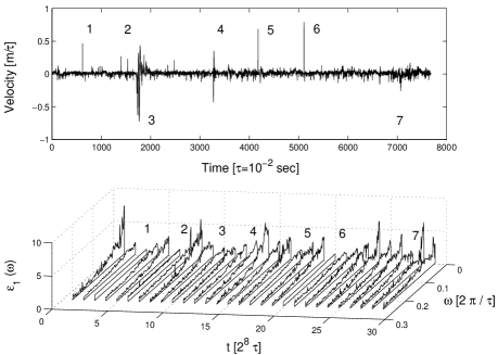
Figure 6: The initial signal - the change of tremor velocity when the second patient is treated by two methods - and the window-time behaviour of the first point of the non-Markovity parameter $\varepsilon_{1}(\omega)$. At the time of a sharp change of the mode (sharp increase of the tremor velocity) in the behaviour of the initial time series (regions 1-7) a gradual decrease of the non-Markovity parameter down to a unit value (the $3rd,6th,10th,14th,17th,20th,27th$ windows) is observed. The decrease of the non-Markovity parameter begins 2-2,5s earlier that the tremor acceleration on an initial series

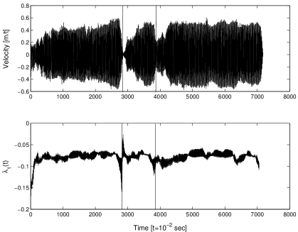
Figure 7: The change of the tremor velocity for the second patient (stimulation of the brain and medication are not used) and the time dependence of the local relaxation parameter $\lambda_{1}(t)$. The localization procedure allows one to find sudden changes of relaxation regimes of the systems under consideration. The largest amplitude values of the local relaxation parameter are in the region of the lowest tremor velocity. The change of the time behaviour of the parameter $\lambda_{1}(t)$ begins 2-3s earlier than the sharp change of the regimes in the initial time series appears

The idea behind the second procedure is the following: one can consider the initial data set and take an N-long sampling. We can calculate kinetic and relaxation parameters for the given sampling. Then we can carry out a ”step-by-step shift to the right”. Then we calculate kinetic and relaxation parameters. After that we execute one more ”step-by-step shift to the right” and continue the procedure up to the end of the time series. Thus, the local averaged parameters have a high sensitivity to the effects of intermittency and non-stationarity. Any non-regularity in the initial time series is instantly reflected in the behaviour of the local average parameters. The optimal length of the sample is 120 points. In Figs. 7, 8 the initial time record and the time dependence of the local relaxation parameter $\lambda_{1}(t)$ are shown in two cases. The change in the time behaviour of the parameter $\lambda_{1}(t)$ begins 2-3s prior to the change of the regimes of the time record of the tremor velocity. The increase of speed of the local relaxation parameter $\lambda_{1}(t)$ testifies to a decrease of tremor velocity.

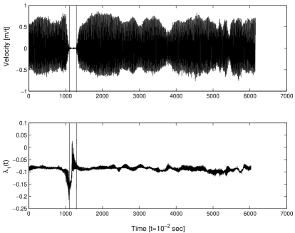
Figure 8: The change of the tremor velocity for the second patient (15 minutes after the stimulator was switched off, medication off) and the time dependence of the local relaxation parameter $\lambda_{1}(t)$. The site characterizing the minimal tremor velocity is allocated. The increase and decrease of the local relaxation parameter occurs 2.5s before the decrease or increase of the tremor velocity. The similar behaviour of the parameter $\lambda_{1}(t)$ can be explained by its high sensitivity to the presence of nonstationarity of the initial signal

7 Conclusions

In this chapter we have proposed a new concept for the study of manifestations of chaoticity. It is based on the application of the statistical non-Markovity parameter and its spectrum as an informational measure of chaoticity. This approach allows one to define the difference between a healthy person and a patient by means of the numerical value of the non-Markovity parameter. This observation gives a reliable tool for the strict quantitative estimates that are necessary for the diagnosis and the quantification of the treatment of patients. As an example we have considered the changes of various dynamic conditions of patients with Parkinson’s disease. The quantitative and qualitative criteria used by us for the definition of chaoticity and regularity of investigated processes in live systems reveal new informational opportunities of the statistical theory of discrete non-Markov random processes. The new concept allows one to estimate quantitatively the efficacy and the quality of the treatment of different patients with Parkinson’s disease. It allows one to investigate various dynamic states of complex systems in real time.

The statistical non-Markovity parameter $\varepsilon_{1}(0)$ can serve as a reliable quantitative informational measure of chaoticity. It allows one to use $\varepsilon_{1}(0)$ for the study of the behaviour of different chaotic systems. In the case of Parkinson’s disease the change of the parameter defines the change of a quantitative measure of chaosity or regularity of a physiological system. The increase of chaoticity reflects the decrease of the quantitative measure of pathology and the improvement of the state of the patient. The increase of the regularity defines high degree of manifestation of pathological states of live systems. The combined power spectra of the initial TCF $\mu_{0}(\omega)$, the three memory functions of junior orders and the frequency dependence of the non-Markovity parameter compose an informational measure which defines the degree of pathological changes in a human organism.

The new procedures (the window-time procedure and the local averaging procedure) give evident predictors of the change of the initial time signal. The window-time behaviour of the non-Markovity parameter $\varepsilon_{1}(\omega)$ reflects the increase of the tremor velocity 2-2.5s earlier. It happens when the non-Markovity parameter approaches a unit value. The procedure of local averaging of the relaxation parameter $\lambda_{1}(t)$ reflects the relaxation changes of physiological processes in a live system. The behaviour of the local parameter $\lambda_{1}(t)$ reacts to a sudden change of relaxation regimes in the initial time record 2-3s earlier. These predictors allow to lower the probability of ineffective use of different methods of treatment.

In the course of the study we have come to the following conclusions:
- The application of medication for the given group of patients proved to be the most efficient way to treat patients with Parkinson’s disease. Used separately stimulation is less effective than the the use of medication.
- The combination of different methods (medication plus electromagnetic stimulator) is less effective than the application of medication or of stimulation. In some cases the combination of medication and stimulation exerts a negative influence on the state of the subject.
- After the stimulator is switched off its aftereffect has an oscillatory character with a low characteristic frequency corresponding to a period of 30 min.
- The efficacy of various medical procedures and the quality of a treatment can be estimated quantitatively for each subject separately with utmost precision.
- However, if we take both chaotic and physiological components into account, the general estimation of the quality of treatment will be more universal. The combination of two methods (DBS and medication, $Q_{T}=4.071$) produces the most effective result in comparison with the effect of DBS (3.661) or of medication (2.883) given separately. This is connected with additional aspect of the estimation of the quality of treatment due to the study both of both chaotic and diagnostic components of a live system. This conclusion corresponds to the results of Beuter1 .

In conclusion we would like to state that our study gives a unique opportunity for the exact quantitative description of the states of patients with Parkinson’s disease at various stages of the disease as well as of the treatment and the recovery of the patient. On the whole, the proposed concept of manifestations of chaoticity opens up great opportunities for the alternative analysis, diagnosis and forecasting of the chaotic behavior of real complex system of live nature.

8 Acknowledgements

This work supported by the RHSF (Grant No. 03-06-00218a), RFBR (Grant No. 02-02-16146) and CCBR of Ministry of Education RF (Grant No. E 02-3.1-538). The authors acknowledge Prof. Anne Beuter for stimulating criticism and valuable discussion and Dr. L.O. Svirina for technical assistance.

References

- (1) S. Boccaletti, C. Grebogi, Y.-C. Lai et. al: Phys. Reports 329, 103 (2000)
- (2) H. Touchette, S. Lloyd: Physica A 331, 140 (2004)
- (3) K. Pyragas: Phys. Lett. A 170, 421 (1992)
- (4) E.R. Hunt: Phys. Rev. Lett. 67, 1953 (1991)
- (5) V. Petrov, V. Gaspar, J. Masere et. al: Nature 361, 240 (1993)
- (6) B.B. Plapp, A.W. Huebler: Phys. Rev. Lett. 65, 2302 (1990)
- (7) W. Just, H. Benner, E. Reibold: Chaos 13, 259 (2003)
- (8) R. Lima, M. Pettini: Phys. Rev. A 41, 726 (1990)
- (9) Y. Braiman, J. Goldhirsch: Phys. Rev. Lett. 66, 2545 (1991)
- (10) R.M. Yulmetyev, P. Hänggi, F.M. Gafarov: Phys. Rev. E 62, 6178 (2000)
- (11) R.M. Yulmetyev, P. Hänggi, F. Gafarov: Phys. Rev. E 65, 046107 (2002)
- (12) R.M. Yulmetyev, F.M. Gafarov, P. Hänggi et. al: Phys. Rev. E 64, 066132 (2001)
- (13) R.M. Yulmetyev, S.A. Demin, N.A. Emelyanova et. al: Physica A 319, 432 (2003)
- (14) R.M. Yulmetyev, N.A. Emelyanova, S.A. Demin et. al: Physica A 331, 300 (2003)
- (15) A. Beuter, M. Titcombe, F. Richer et. al: Thalamus & Related Systems 1, 203 (2001); M. Titcombe, L. Glass, D. Guehl et. al: Chaos 11, 766 (2001)
- (16) A. Beuter, A. de Geoffroy, P. Cordo: J. Neurosci. Meth. 53, 47 (1994)
- (17) K.E. Norman, R. Edwards, A. Beuter: J. Neurosci. Meth. 92, 41 (1999)
- (18) R.M. Yulmetyev, P. Hänggi, F.M. Gafarov: JETP 123, 643 (2003)