Functional dissipation microarrays for classification
Abstract
In this article, we describe a new method of extracting information from signals, called functional dissipation, that proves to be very effective for enhancing classification of high resolution, texture-rich data. Our algorithm bypasses to some extent the need to have very specialized feature extraction techniques, and can potentially be used as an intermediate, feature enhancement step in any classification scheme.
Functional dissipation is based on signal transforms, but uses the transforms recursively to uncover new features. We generate a variety of masking functions and ‘extract’ features with several generalized matching pursuit iterations. In each iteration, the recursive process modifies several coefficients of the transformed signal with the largest absolute values according to the specific masking function; in this way the greedy pursuit is turned into a slow, controlled, dissipation of the structure of the signal that, for some masking functions, enhances separation among classes.
Our case study in this paper is the classification of
crystallization patterns of amino acids solutions affected by the
addition of small quantities of proteins.
Keywords: Features enhancement, matching pursuit,
classification, non-linear iterative maps, wavelet transforms.
1 Introduction
In this paper we introduce the functional dissipation microarray, a feature enhancement algorithm that is directly inspired by experimental microarray techniques [1]. Our method shows how ideas from biological methodologies can be successfully turned into functional data analysis tools.
The idea behind the use of microarrays is that if a large and diverse enough data set can be collected on a phenomenon, it is often possible to answer many questions, even when no specific interpretation for the data is known. The algorithm we describe here seems particularly suitable for high resolution, texture-rich data, and bypasses to some extent the need to preprocess with specialized feature extraction algorithms. Moreover, it can potentially be used as an intermediate feature enhancement step in any classification scheme.
Our algorithm is based on an unconventional use of matching pursuit ([2], Chapter 9; [3]). More precisely, we generate random masking functions and ‘select’ features with several generalized matching pursuit iterations. In each iteration, the recursive process modifies several of the largest coefficients of the transformed signal according to the masking function. In this way the matching pursuit becomes a slow, controlled dissipation of the structure of the signal; we call this process functional dissipation. The idea is that some unknown statistical feature of the original signal many be detected in the dissipation process at least for some of the random maskings.
This process is striking in that, individually, each feature extraction with masking becomes unintelligible because of the added randomness and dissipation, and only a string of such feature extractions can be ‘blindly’ used to some effect. There is some similarity in spirit between our approach and the beautiful results on random projections reconstructions described in [4] and [5], with the important difference that we use several distinct randomization and dissipation processes to our benefit so that there is a strong non-linear dynamics emphasis in our work. Moreover, we bypass altogether reconstruction issues, focusing directly on classification in the original representation space. Our method can be seen also as a new instance of ensemble classifiers (like boosting [6] and bagging [7]), in that several functional dissipations are generally pulled together to achieve improvement of classification results.
Other applications of matching pursuit to classification problems include kernel matching pursuit methods [8], and also boosting methods, that can be interpreted essentially as greedy matching pursuit methods where the choice of ‘best’ coefficient at each iteration is made with respect to more sophisticated loss functions than in the standard case (see [9], [10], [11] chapter 10). We stress again that, while our approach uses the structure of matching pursuits, only their rich dynamical properties (highlighted for example in [3]) are used for the generation of features, since in our method the whole iterative process of modifying coefficients becomes simply an instance of non-linear iterative maps, disjoined from approximation purposes.
The case study of this paper is the classification of crystallization patterns of amino acids solutions affected by addition of small quantities of proteins; such crystallization patterns show varied and interesting textures. The goal is to recognize whether an unknown solution contains one of several proteins in a database. Crystallization patterns may be significantly affected by laboratory conditions, such as temperature and humidity, so the degree of similarity of patterns belonging to a same protein is subject to some variations, adding difficulty to the classification problem. The richness of the textures and their variability gives this classification problem an appeal that goes beyond the specific application from which it arises.
Our basic approach is to derive long feature vectors for each amino acid reporter by our generalized recursive greedy matching pursuit. Since the crystallization patterns are generated by stochastic processes, there is a great local variability in each droplet and any significant feature must encode a statistical information about the image to be part of a robust classifier, see [10]. We can see this case study as an instance of texture classification, and it is well established that wavelets (see [2] chapter 5, [13]) and moments of wavelet coefficients (see [14], or [15] for the specific problem of iris recognition) can be very useful for these types of problems. Therefore we implemented our method in the context of a wavelet image transform for this case study, even though we then summarized the information obtained with the functional dissipation with moments of the dissipated images in the original representation space. Other choices of statistical quantities are possible in principle according to the specific application, since, as we show in section 2, the method can be formulated in a quite general setting.
In section 2 we introduce the features enhancement method, functional dissipation, to explore the feature space. In sections 3 and 4 we apply the method to the crystallization data to show how the application of a sufficiently large number of different functional dissipations can greatly improve the classification error rates.
2 Functional dissipation for classification
In this section we introduce a classification algorithm that is designed for cases where feature identification is complicated or difficult. We first outline the major steps of the algorithm, and then discuss specific implementations. In the following sections we apply one possible implementation of this method to droplet classification, and describe the results.
We begin with input data divided into a training set and a test set. We then follow four steps as follows:
-
A
Choose a classifier and a figure of merit that quantifies the classification quality.
-
B
Choose a basic method of generating features from the input data, and then enhance the features by a recursive process of structure dissipation, described below.
-
C
Compute the figure of merit from A for all features derived in B. For a fixed integer , search the feature space defined in B for the features which maximize the figure of merit in A on the training set.
-
D
Apply the classifier from A, using the optimal features from C, to classify the test set.
In step A, for example, multivariate linear discrimination can be used as a classifier. This method comes with a built-in figure of merit, the ratio of the between-group variance to the within-group variance. More sophisticated classifiers often have closely associated evaluation parameters. Cross-validation or leave-one-out error rates can be used.
Step B is the heart of the functional dissipation algorithm. The features used will depend on the problem. For two-dimensional images, orthogonal or over-complete image transforms can be used. The method of functional dissipation is a way to leverage the extraction of general purpose features to generate features with increased classification power. This method uses the transforms recursively to gradually modify the feature set.
Consider a single input datum and several invertible transforms , , that can be applied to (in the case study to be shown later, represents a gray scale image and represent Discrete Wavelet Transforms). At each iteration we select several coefficients from the input datum and we use the mask to modify the coefficients themselves. Fix positive integers and set Let be a discrete valued function defined on , which we call a mask or a masking function. Apply the following functional dissipation steps (B1)-(B3) times. For :
(B1): Compute the transform
(B2): Choose a subset of and collect the coefficients , in with largest absolute value in a suitable subset.
(B3): Apply the mask: Set , and modify the corresponding coefficients of in the same fashion. Set to be the inverse of the modified coefficients .
At the conclusion of the steps, features are generated by computing statistics that describe the probability distribution of , . For example, one could use , , the third and fourth moments of the set (or even more moments for large images). These statistics are used as features, delivered by the means of functional dissipation. If we carry out these steps for different masks , we obtain a -dimensional feature vector for each data input (where we counted the moments of the input images only once).
One way to view our approach is as a matching pursuit strategy (see [2] chapter 9), but used in a new and unusual way. In general, matching pursuit is used to find good suboptimal approximations to a signal. The way this is done is by expanding a function in some dictionary and by choosing the element in the dictionary for which is maximum. Given an initial approximation of , and an initial residue , we set and . The process is repeated on the residue several times to extract successively different relevant structures from the signal.
Instead, in each iteration of our algorithm we modify several of the largest coefficients in different regions of the transformed signal according to the random masking functions, so that only the non-linear interaction of the signal and the masking function is of interest and not the approximation of the underlying signal. The residue is perturbed more and more until, in the limit, no structure of the original signal is visible in either and . This is therefore a slow, controlled dissipation of the structure of the signal. Note that the structure of the signal is dissipated, not its energy, in other words the images are allowed in principle to increase in norm as .
We can think of the input image as initial condition of the iterative map defined by mask and dissipation, and the application of several dissipation processes allows to identify those maps for which different classes of images flow in different regions of the feature space as defined by the output of the map. It seems likely that, for some non-linear maps, similar initial conditions will evolve with similar dynamics, while small differences among classes will be enhanced by the dynamics of the map and therefore they will be detectable as the number of iterations increase. The key question is whether a small set of masks can generate enough variability among the dissipative processes to find such interesting dynamics. Our results show that, for our case study, this is the case. According to this qualitative dynamical system interpretation, our method can be seen along the lines of dynamical system algorithms for data analysis such as those developed in [16] to approach numerical linear algebra problems.
In choosing the masking functions for (B1)-(B3), the guiding idea is to have large variability in the masks themselves so that there is a wide range of possible dynamics in the dissipations processes, while at the same time preserving some of the structure of the signal from one iteration to the next (in other words we want the signals to be dissipated, but slowly). To this extent, the masking functions are designed to assume small values so that the image is only slightly affected at each iteration by the change of of a subset of its coefficients as in (B1)-(B3). To respect these limitations, we decided to take each mask as a realization of length of Gaussian white noise with variance , we then convolve it with a low-pass filter to increase smoothness and finally we rescale it to have a fixed maximum absolute value.
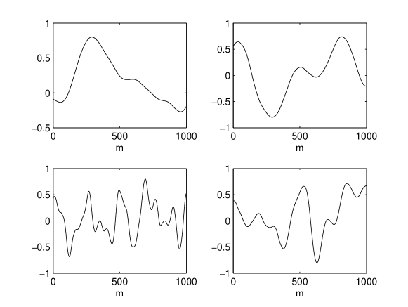
More precisely, let , be a realization of Gaussian white noise of length , and let be a smoothing filter defined on all integers such that where denotes the function that assumes value for and value otherwise (we follow here [2] page 440). Let now be the convolution of and , where is suitably extended periodically at the boundary. Then each mask can be written as , where is a small real number. The larger , the smoother the mask , but the fact that each underlying is a random process assures the necessary variability. We repeat this process times choosing several values of and to generate curves of the type shown in Figure 1.
Remark 1: For our case study in section 3, we choose to be distributed on , and we choose a logarithmic distribution on this set so that smoother masks are favored. Specifically we take and uniformly in the set . We choose (specifically, ) to cause slow dissipation.
The randomness of the specific choice of masks is used to allow a wide spanning of possible mask shapes, and we expect more general classes of maskings to be suitable for this method. On the other hand the question of which is the smallest class of masks that allows effective feature extraction is still open.111A patent application has been filed on the method described in this paper with U.S. Provisional Patent Application Number 60/687,868, file date 6/7/2005..
3 Case Study: Droplet Classification
In this section we describe the case study that motivated this research, the classification of proteins by their effect on crystallization patterns of amino acids used as reporter substances. We restrict ourselves to a database of four classes : proteins and control. The proteins are albumin from chicken egg white, hemoglobin from bovine blood and lysozyme, which we denote respectively as , and respectively. These proteins were added to solutions of one amino acid, namely leucine, denoted by . The control solution without protein will be denoted as . Both the number of proteins to classify and the number of reporters can increase in practice, but we restrict our analysis to this smaller set for our purposes as already with these few classes of proteins we can see the basic difficulty of distinguishing even by eye some of the patterns.
A crucial advance in the experimental study of droplets has been the ability to generate quickly a large number of droplets to which different amino acids have been added. Remarkably, the addition of proteins to the amino acid reporters can have very different effects on the crystallization patterns. In some cases there is no visible difference between droplets of amino acid plus (control) and droplets of amino acid plus protein; for some other proteins the resulting crystallization patterns are very different from control [17]. Clearly the different behavior of solutions for different amino acids can greatly facilitate classification.
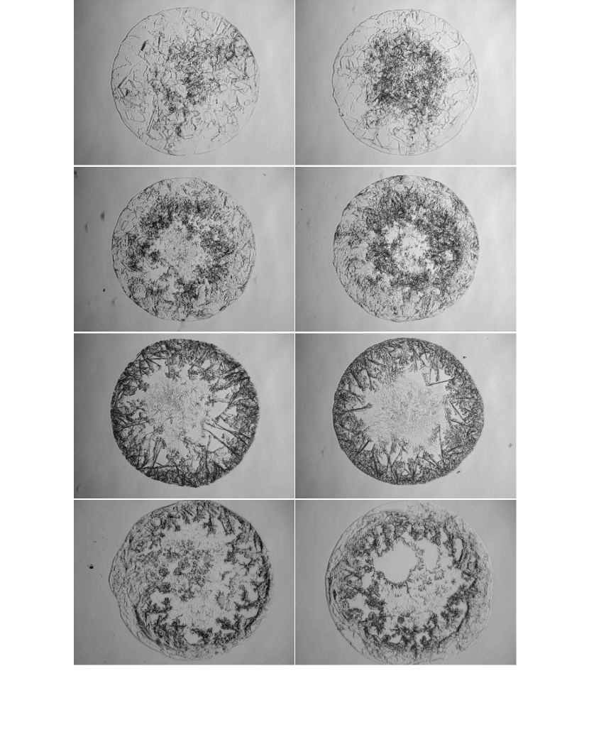
In Figure 2, each row shows two representative patterns of the amino acid solutions with the three proteins , , and added. Note in particular that the appearance of droplets for and show several similarities (for example large, glassy crystals at the boundary) and that there is a significant degree of variability within each class.
4 Results and Discussion
In this section we discuss a particular implementation of the pattern classification algorithm of Section 2, and the results of applying it to the droplets. We used for our analysis 20 gray-scale images of crystallization patterns for each combination of amino acid , with proteins ,, and with . For each droplet , i.e. the -th image instance of protein with addition of amino acid , we reduce the size of the image to a matrix of by pixels and we normalize the image so that its mean as an array is zero and its variance is one.
For purposes of comparison, we will apply the steps (B1)-(B3) in several ways. First we set the number of iterations of the dissipation to zero (), and we apply the process only once, which corresponds to a direct evaluation of the moments of the images. Then we apply the algorithm choosing the best features with several masks and no dissipation () and with several masks and function dissipation (). The masking functions we use are the Gaussian processes described at the end of section 2 with parameters as in remark 1. Subsequently we use, for the case and , a larger number of features (namely , one for each distinct pair of classes), and we show that error rates are very low in this setting when .
In all cases we apply to the selected features a general purpose classification algorithm such as a 3-nearest neighborhood (3-NN) classifier to the output of (B1)-(B3) and we test each case by dividing the instances of feature vectors for each class randomly into a training set of instances and a test set of instances. We train the classifier on the training set and then test it on the remaining instances of each class. Note that we are interested in identifying each distinct protein and control reporters as well, so the total number of classes that we try to discriminate are , i.e. the three proteins and .
We repeated each classification scheme times, using different divisions into training and testing sets to obtain estimated of the misclassification error rates for each class.
The transforms in steps (B1)-(B3) are set to be the discrete wavelet transform with Daubechies mother wavelet ( vanishing moments). The restricted subset of action (as in (B2)) is the detail level at scale (highlighting intermediate scale details of the image) for even and the detail level at scale (fine scale details) for odd (see [2] section 7.7 for more on two dimensional orthogonal wavelet bases).
Remark 2:The signal transforms need to be selected according to the specifics of the problem. The potential of our method is that the features exploration performed by functional dissipation utilizes variations of general purpose signal transforms, avoiding the need to exactly adapt the transform to the characteristics of the classes of signals.
Remark 3:Moments of images for large iterations can show sometimes a very distinct order of magnitude for different classes. While this is good in general for classification, it is not so good for selecting suitable ‘best’ features. The reason is that the differences among some of the classes can be flattened if they are very close with respect to other classes. Therefore we take the logarithm of the absolute value of moments in all the following classification schemes, and we scale them to have joint variance and mean .
First, with no dissipation or coefficient masking occurs. For each droplet image a two dimensional feature vector is extracted with (B1)-(B3) by computing the log of the norm of the third and forth moments of the images. The 3-NN classifier trained on these features achieves classification with a low degree of accuracy especially for : the estimated misclassification errors for the three test proteins and are: for ; for for and for . This poor classification is not surprising as statistics of images before a suitable image transform are generally considered a weak classifier.
Second, we now take random functions , defined on as in section 2. For each we apply steps (B1)-(B3) with iterations and we select coefficients. The repeated use of (B1)-(B3) for each masking gives a -dimensional feature vector for each image droplet (we counted only one time the moments of the input images). We select now the ‘best’ features (say for example to be consistent with the previous case) for which the ratio of between-class variance over within-class variance for the training sets were maximal (see [11] page 94 for more on such notion).
If we use only these features in the 3-NN classification of the test sets, then the estimated misclassification errors for the four classes are: for ; for for and for . Not only there is no improvement over the case , but results significantly worsen for and (this is so even when we let increase). This is at first sight puzzling as we are using also the features collected in the case , but the features selection may well choose a feature that has better separation for some classes, but worse for others. For other tests sets we did not observe such peculiar phenomenon, but the error rates are consistently of the same order of the case .
Third, we take random masks , defined on as in section 2 and we now turn on the function dissipation technique by setting in the steps (B1)-(B3). At each iteration we select coefficients. If we repeat (B1)-(B3) for each masking , we obtain a -dimensional feature vector for each image droplet. We select now the ‘best’ features for which the ratio of between-class variance over within-class variance for the training sets were maximal. If we use only these moments in the 3-NN classification of the test sets, then the estimated misclassification errors for the four classes are:for ; for for and for . For and , this is an excellent improvement with respect to the feature selection based on logarithms of moments of the original images (the first case we considered with ), while errors are of the same order for and .
The progression from to shows in a compelling way that both masking function and dissipation are essential ingredients of the method to improve error rates and masking alone (which can be seen as a type of nonlinear projection) is not sufficient, or may actually, in some cases, be harmful by itself for classification.
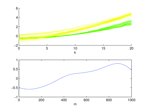
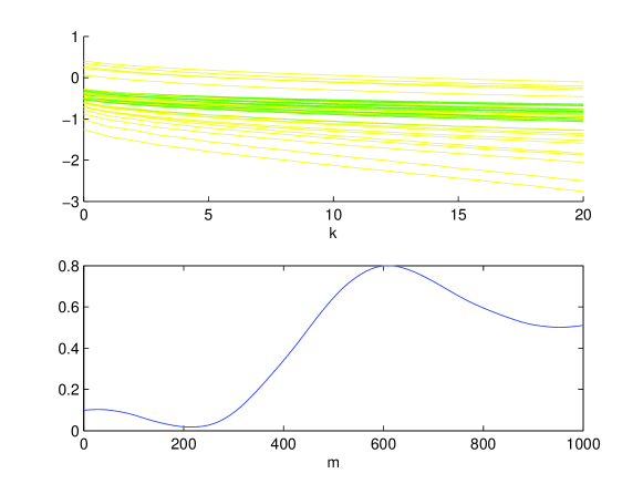
In Figure 3 we show the third moment (skewness) for the instances of (in green) and the instances of (in yellow), as we move along the dissipation process for one specific mask that shows improved separation among these two classes. At we pictured the moment distribution of the images when no mask and no dissipation is applied. Note that there is no good separation between these classes for , then finally we start to see a divergence of the clusters of moments and for we observe significant separation of the classes, the bottom subplot shows the shape of the corresponding mask. This distinct improvement of separation with tightly clustered classes happens, with similar dynamics, for 22 out of the 100 masks that we generated, while for the remaining masks we have no improvement in separation as shown in Figure 4 or we have poorly clustered classes. Interestingly, most (but not all) of the masks that show improved separation between and assume negative values for for the first few hundred largest coefficients. This generic shape would have been difficult to predict, but is simple enough that it raises the hope that spanning a small space of masks will be enough in general classification problems, greatly reducing the training computational cost, but it is likely that thousands of masks may be necessary for very difficult classification problems. Note that, for different pairs of classes, the masks that improve separation may have very different shapes, for example, separation between and is particularly improved by some masks that assume negative values for the middle range coefficients and the total number of masks for which we have improved separation with tight clusters is smaller in this case, 13 masks out of 100. We will use now this last observation to lower even further the classification error rates.
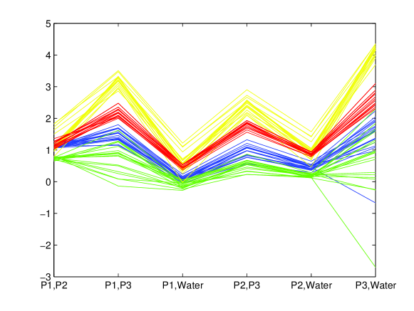
The classification with masks and iterations significantly improved error rates, but we still had a roughly error rate for and . If we relax the artificial restriction that only best features are extracted we can greatly improve on this result. More specifically suppose we extract one best feature for each pair of classes, and let be such feature (we have a total of such features for a 4 classes problem). The best features for each pair of classes are shown in Figure 5. Within the setting of the previous classification schemes, apply to each testing image a 3-NN classification for feature using only classes and and repeat the classification for each of the features. Finally use a majority vote among all classifications to assign a class to each testing image. With the same masks and iterations as in the previous cases the estimated error rate are now: for ; for for and for . If we take only the errors are instead large:for ; for for and for . With both large number of masks and dissipation turned on there is virtually no misclassification. This raises the issue of whether we are overfitting the data, so as a final test of the method, we mixed randomly all images from all classes, we divided them in four sets of 20 images each and then we applied to these four pseudo-classes the features classification that we just described. In this case no mask among those that we generated and no dissipation process is able to improve classification results, which are consistently very poor exactly as we would expect. We summarize our results for the classification schemes that we used in Table 1.
| Class | K=0 p=2 | K=1 p=2 | K=20 p=2 | K=1 p=6 | K=20 p=6 |
|---|---|---|---|---|---|
The use of many masks allow to look at data from many different (albeit unstructured) view points: in line with microarray approach, we suggestively call each of the elements of the feature vector a dissipative gene. When we display the resulting dissipative genes in several columns, each column representing the dissipative genes for one instance of a protein or , we have what we can properly call a functional dissipation microarray. In is interesting to note that, supposedly, one of the weaknesses of matching pursuit is its inability, as a greedy algorithm, to find an optimal representation for a given signal; the use of randomization and dissipation turns this weakness in a strength, at least in the setting of classification problems. This change of perspective is in line with the idea that greedy matching pursuit methods have a greater potential than simply being approximations to optimal solutions. The dynamical interaction of masks and dissipative iterations makes the signals ‘flow’ in the feature space and it is this flow that often carries the most significant information on the initial conditions and therefore on the signals themselves.
Acknowledgments
The authors gratefully acknowledge support from DOE grant, DE-F C52-04NA25455. We also thank the anonymous referee for very useful and constructive remarks.
References
- [1
-
] P. Baldi, G. W. Hatfield, W. G. Hatfield, DNA Microarrays and Gene Expression : From Experiments to Data Analysis and Modeling. Cambridge University Press (2002).
- [2
-
] S. Mallat, A Wavelet Tour of Signal Processing, Academic Press (1998).
- [3
-
] G. Davis, S. Mallat and M. Avelaneda, Adaptive Greedy Approximations, Jour. of Constructive Approximation, 13 1997 (1), pp. .
- [4
-
] E. J. Candes and J. Romberg, Practical Signal Recovery from Random Projections, Wavelet Applications in Signal and Image Processing XI, Proc. SPIE Conf. vol. 5914 (2005), 59140S.
- [5
-
] E. J. Candes, J. Romberg and T. Tao, Robust uncertainty principles: exact signal reconstruction from highly incomplete frequency information. IEEE Trans. Inform. Theory, 52 (2004) 489-509.
- [6
-
]Y. Freund, R. Schapire, A short introduction to boosting, J. Japan. Soc. for Artifcial Intelligence, vol. 14 n. 5 (1999), pp. .
- [7
-
] L. Breiman. Bagging predictors. Machine Learning, 24 (1996), pp. .
- [8
-
] P. Vincent, Y. Bengio, Kernel matching pursuit, Mach. Learn. J. 48 (2002) (1), pp. .
- [9
-
] J. Friedman, T. Hastie, R. Tibshirani, Additive Logistic Regression : a Statistical View of Boosting, Annals of Statistics, 28 (2000), pp. .
- [10
-
] J. Friedman, Greedy function approximation: A gradient boosting machine. Ann. Statist. 29 (2001) (5), pp. .
- [11
-
] T. Hastie, R. Tibshirani, J. Friedman, The elements of Statistical Learning, Springer (2001).
- [12
-
] K. Fukunaga. Introduction to Statistical Pattern Recognition (2nd Edition ed.), Academic Press, New York (1990).
- [13
-
] A. Laine and J. Fan, Texture classification by wavelet packet signatures. IEEE Trans. Pattern Anal. Mach. Intell. 15 11 (1993), pp. .
- [14
-
] Q. Jin and R. Dai, Wavelet invariants based on moment representation, Pattern Recognition Artif. Intell. 8 (1995) (3), pp. .
- [15
-
] S. Noh, K. Bae, Y. Park, J. Kim, A Novel Method to Extract Features for Iris Recognition System. AVBPA 2003, LNCS 2688 (2003), pp. .
- [16
-
] R.W. Brockett, Dynamical systems that sort lists, diagonalise matrices, and solve linear programming problems. Lin. Algebra Appl. 146 (1991), pp. .
- [17
-
] V. N. Morozov, N. N. Vsevolodov, A. Elliott, C.Bailey, Recognition of Proteins by Crystallization Patterns in an Array of Reporter Solution Microdroplets, Anal. Chem. vol. 78 (2006), pp. .