Generalized Permeability Function and Field Energy Density in Artificial Magnetics Using the Equivalent Circuit Method

Abstract

The equivalent circuit model for artificial magnetic materials based on various arrangements of split rings is generalized by taking into account losses in the substrate or matrix material. It is shown that a modification is needed to the known macroscopic permeability function in order to correctly describe these materials. Depending on the dominating loss mechanism (conductive losses in metal parts or dielectric losses in the substrate) the permeability function has different forms. The proposed circuit model and permeability function are experimentally validated. Furthermore, starting from the generalized circuit model we derive an explicit expression for the electromagnetic field energy density in artificial magnetic media. This expression is valid at low frequencies and in the vicinity of the resonance also when dispersion and losses in the material are strong. The presently obtained results for the energy density are compared with the results obtained using different methods.

I Introduction

Artificial electromagnetic media with extraordinary properties (often called metamaterials) attract increasing attention in the microwave community. One of the widely studied subclasses of metamaterials are artificial magnetic materials operating in the microwave regime, e.g. [1]–[8]. Broken loops have been used as one of the building blocks to implement double-negative (DNG) media [9, 10], in addition to this, artificial magneto-dielectric substrates are nowadays considered as one of the most promising ways to miniaturize microstrip antennas [11]–[17].

The extraordinary features of metamaterials call for careful analysis when studying the fundamental electromagnetic quantities in these materials. Recently, a lot of research has been devoted to the definition of field energy density in DNG media [18]–[21]. Authors of [18, 19, 21] derived the energy density expression starting from the macroscopic media model and writing down the equation of motion for polarization (electric charge) or magnetization density in the media. Furthermore, complex Poynting theorem was used to search for expressions having the mathematically correct form to be identified as energy densities. Following the terminology presented in [21] we call this method “electrodynamic method” (ED). Tretyakov used in [20] another method: Starting from the material microstructure, an equivalent circuit representation was derived for the unit cell constituting specific artificial dielectric and magnetic media. Lattices of thin wires and arrays of split-ring resonators were considered in [20]. The stored reactive energy, and, furthermore, the field energy density, were calculated using the classical circuit theory. Authors of [21] later called this method “equivalent circuit method” (EC). Though these two methods apply to media with the same macroscopic permeabilities and permittivities, they are fundamentally very different, as will be clarified later in more detail. Moreover, the final expressions for the field energy density in artificial magnetic media given in [20] and [21] differ from each other. One of the motivations of this work is to clarify the reasons for this difference.

Here we concentrate only on artificial magnetic media and set two main goals for our work: 1) To understand the differences and assumptions behind the ED and EC-methods when deriving the field energy density expressions. We verify using a specific example (magnetic material unit cell) that in the presence of non-negligible losses one always should calculate the stored energy at the microscopic level. 2) To generalize the previously reported equivalent circuit representation for artificial magnetic media [20]. The generalized circuit model takes into account losses in the matrix material. It is shown that this generalization forces a modification to the widely accepted permeability function used to macroscopically describe artificial magnetic media. The generalization has a significant importance as it is shown that in a practical situation matrix losses strongly dominate over conductive losses. The proposed circuit representation and permeability function are experimentally validated: We measure the magnetic polarizability of a small magnetic material sample and compare the results with those given by the proposed analytical model and the previously used model. The results given by the proposed model agree very well with the measured results, whereas the old model leads to dramatic overestimation for the polarizability. Using the generalized circuit model we derive an expression for the field energy density in artificial magnetic media. This expression is compared with the results obtained using the ED-method in [21]. Reasons for the differences in the results are discussed.

II Electrodynamic method vs. Equivalent circuit method

It is well explained in reference books (e.g. [22, 23]) that for the definition of field energy density in a material having non-negligible losses one always needs to know the material microstructure. First of all, the reactive energy stored in any material sample is a quantity that can be measured. When the material is lossless, no information is needed about the material microstructure for this measurement. Indeed, we can measure the total power flux through the surface of sample volume and, since there is no power loss inside, we can use the Poynting theorem to determine the change in the stored energy. This is the reason why the field energy density in a dispersive media with negligible losses can be expressed through the frequency derivative of macroscopic material parameters. In the circuit theory, the same conclusion is true for circuits that contain only reactive elements: It is possible to find the stored reactive energy in the whole circuit knowing only the input impedance of a two-pole [24].

Simple reasoning reveals, that in the presence of non-negligible material losses the above described “black box” representation and direct measurement are not applicable: Without knowing the material microstructure or the circuit topology we do not know which portion of the input power is dissipated and which is stored in the reactive elements. Thus, the energy stored in a lossy media cannot be uniquely defined by only utilizing the knowledge about the macroscopic behavior of the media [22, 23].

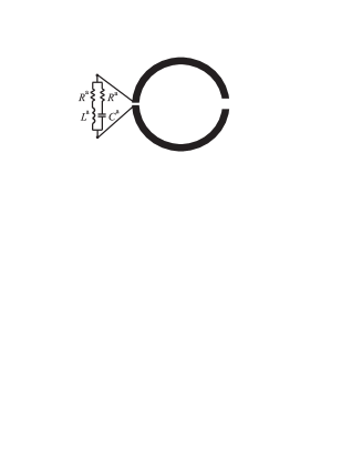
Figure 1: Split-ring resonator loaded with an infinitesimally small lumped circuit.

When defining the energy density in a certain material using the ED-method one first writes down the equation of motion for charge density or for magnetization in the medium using the macroscopic media model [19, 21]. We stress that this equation is the macroscopic equation of motion, containing the same physical information as the macroscopic permittivity and permeability. Further, complex Poynting theorem is used to identify the mathematical form of the general macroscopic energy density expressions. Having the form of these expressions in mind one searches for similar expressions in the equation of motion and defines them as energy densities. The problem of the ED-method method is the fact that it only utilizes the knowledge about the macroscopic behavior of the media, which, as explained above, in not enough. The aforementioned difficulty is avoided in the EC-method [20]. Based on the known microscopic medium structure, one constructs the equivalent circuit for the unit cell of the medium. Careful analysis is needed to make sure that the circuit physically corresponds to the analyzed unit cell. After this check the stored reactive energy and the corresponding field energy density can be uniquely calculated using the classical circuit theory.

Next, we illustrate the difference between the ED- and EC-methods using a specific case of split-ring composites. Consider the split-ring resonator (SRR) shown in Fig. 1. Following a example given in [23], we load the SRR with an electrically infinitesimally small circuit consisting of lumped elements. Let us assume that the additional inductance and capacitance are chosen to have values $L^{\rm a}=\tau R^{\rm a},C^{\rm a}=\tau/R^{\rm a},\tau>0$. A simple check reveals that in this case the input impedance of the load circuit is frequency independent and purely resistive: $Z_{\rm in}=R^{\rm a}$. When the SRR is electrically small, it can be represented as a resonant contour and the total loss resistance reads $R_{\rm tot}=R+R^{\rm a}$, where $R$ is the loss resistance due to the finite conductivity of the loop materials. Let us further assume that the ring is made of silver and the value of $R^{\rm a}$ is chosen so that $R_{\rm tot}$ is the same as $R$ for an unloaded SRR made of copper. In this case the macroscopic descriptions of a medium formed by the loaded SRRs made of silver with additional loads and unloaded SRRs made of copper are exactly the same. Thus, the ED-method predicts the same value for the reactive energy stored in these two media. Inspection of Fig. 1 clearly indicates, however, that this is not the case. There is additional energy stored in the load inductance and capacitance, which is invisible on the level of the macroscopic permeability description. Proper definition of the stored energy must be done at the microscopic level, which is possible with the equivalent circuit method.

III Equivalent circuit method: Brief revision of earlier results

A commonly accepted permeability model as an effective medium description of dense (in terms of the wavelength) arrays of split-ring resonators and other similar structures reads

$$\mu(\omega)=\mu_{0}\mu_{\rm r}(\omega)=\mu_{0}\bigg{(}1+\frac{A\omega^{2}}{\omega_{\rm 0}^{2}-\omega^{2}+j\omega\Gamma}\bigg{)}$$ (1)

(see e.g. [1, 2, 4, 8].) Above, $A$ is the amplitude factor ($0<A<1$), $\omega_{\rm 0}$ is the undamped angular frequency of the zeroth pole pair (the resonant frequency of the array), and $\Gamma$ is the loss factor. The model is obviously applicable only in the quasi-static regime since in the limit $\omega\rightarrow\infty$ the permeability does not tend to $\mu_{0}$. At extremely high frequencies materials cannot be polarized due to inertia of electrons, thus, a physically sound high frequency limit is $\mu_{0}$ [22]. However, (1) gives correct results at low frequencies and in the vicinity of the resonance. This is the typical frequency range of interest e.g. when utilizing artificial magneto-dielectric substrates in antenna miniaturization [13, 16, 17]. The other relevant restriction on the permeability function is the inequality [22]

$${\partial(\omega\mu)\over\partial\omega}>\mu_{0},$$ (2)

valid in the frequency regions with negligible losses. Physically the last restriction means that the stored energy density in a passive linear lossless medium must be always larger than the energy density of the same field in vacuum. Macroscopic model (1) violates restriction (2) at high frequencies, which is another manifestation of the quasi-static nature of the model. In the vicinity of the magnetic resonance the effective permittivity of a dense array of split-ring resonators is weakly dispersive, and can be assumed to be constant.

In [20] the energy density in dispersive and lossy magnetic materials was introduced via a thought experiment: A small (in terms of the wavelength or the decay length in the material) sample of a magnetic material [described by (1)] was positioned in the magnetic field created by a tightly wounded long solenoid having inductance $L_{0}$, Fig. 2a. The insertion changes the impedance of the solenoid to

$$Z(\omega)=j\omega{L_{0}}\mu_{\rm r}(\omega)=j\omega{L_{0}}+\frac{j\omega^{3}L_{0}A}{\omega_{\rm 0}^{2}-\omega^{2}+j\omega\Gamma}.$$ (3)

The equivalent circuit with the same impedance was found to be that shown in Fig. 2b [20] with the impedance seen by the source

$$Z(\omega)=j\omega{L_{0}}+\frac{j\omega^{3}M^{2}/L}{\frac{1}{LC}-\omega^{2}+j\omega\frac{R}{L}},$$ (4)

which is the same as (3) if

$$\frac{M^{2}}{LL_{0}}=A,\quad\frac{1}{LC}=\omega_{\rm 0}^{2},\quad\frac{R}{L}=\Gamma.$$ (5)

The aforementioned equivalent circuit model is correct from the microscopic point of view since the modeled material is a collection of capacitively loaded loops magnetically coupled to the incident magnetic field. An important assumption in [20] and in the present paper is that the current distribution is nearly uniform over the loop. This means that the electric dipole moment created by the exciting field is negligible as compared to the magnetic moment. The electromagnetic field energy density in the material was found to be [20]

$$w_{\rm m}=\frac{\mu_{0}}{2}\bigg{(}1+\frac{A\omega^{2}(\omega_{\rm 0}^{2}+\omega^{2})}{(\omega_{\rm 0}^{2}-\omega^{2})^{2}+\omega^{2}\Gamma^{2}}\bigg{)}|H|^{2}.$$ (6)

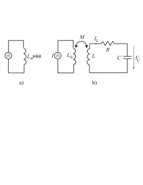
Figure 2: a) Magnetic material sample in the probe magnetic field of a tightly wounded long solenoid. b) Equivalent circuit model, losses in the matrix material are not taken into account.

In [20] only losses due to nonideally conducting metal of loops were taken into account, and losses in the matrix material (substrate material on which metal loops are printed) were neglected. It will be shown below that neglecting the matrix losses can lead to severe overestimation of the achievable permeability values.

IV Generalized equivalent circuit model and permeability function

Losses in the matrix material (typically a lossy dielectric laminate) can be modeled by an additional resistor in parallel with the capacitor. Indeed, if a capacitor is filled with a lossy dielectric material, the admittance reads

$$Y=j\omega{C}(\epsilon^{\prime}-j\epsilon^{\prime\prime})=j\omega{C}\epsilon^{\prime}+\omega{C}\epsilon^{\prime\prime},$$ (7)

where the latter expression denotes a loss conductance. Thus, the microscopically correct equivalent circuit model is that shown in Fig. 3b.

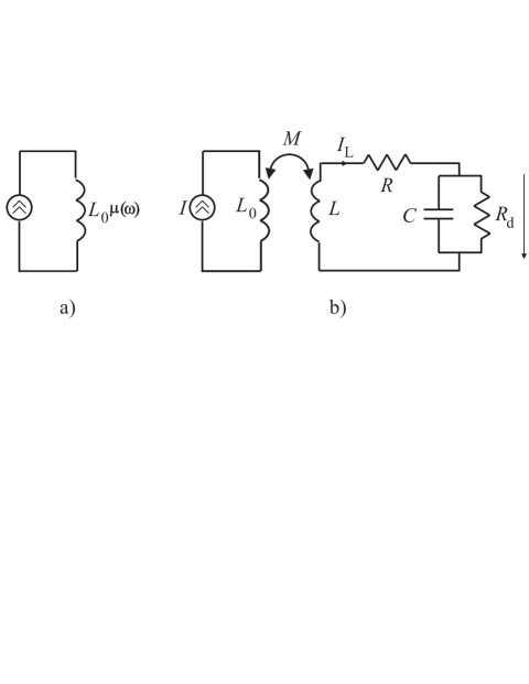
Figure 3: a) Magnetic material sample in the probe magnetic field of a tightly wounded long solenoid. b) Equivalent circuit model taking into account losses in the matrix material.

The impedance seen by the source can be readily solved:

$$Z=j\omega{L_{0}}+\frac{j\omega^{3}M^{2}/L+\omega^{2}M^{2}/(LCR_{\rm d})}{(1+\frac{R}{R_{\rm d}})\frac{1}{LC}-\omega^{2}+j\omega{(\frac{R}{L}+\frac{1}{CR_{\rm d}})}}.$$ (8)

The macroscopic permeability function corresponding to this model reads

$$\mu(\omega)=\mu_{0}\bigg{(}1+\frac{\omega^{2}M^{2}/(LL_{0})-j\omega{M^{2}}/(LL_{0}CR_{\rm d})}{(1+\frac{R}{R_{\rm d}})\frac{1}{LC}-\omega^{2}+j\omega{(\frac{R}{L}+\frac{1}{CR_{\rm d}})}}\bigg{)}.$$ (9)

Comparing (1) and (9) we immediately notice that (1) is an insufficient macroscopic model for the substrate if the losses in the host matrix are not negligible. A proper macroscopic model correctly representing the composite from the microscopic point of view is

$$\mu(\omega)=\mu_{0}\mu_{\rm r}(\omega)=\mu_{0}\bigg{(}1+\frac{A\omega^{2}-j\omega{B}}{\widetilde{\omega}_{\rm 0}^{2}-\omega^{2}+j\omega(\Gamma+\Gamma_{\rm d})}\bigg{)}.$$ (10)

Equation (9) is the same as (10) if

$$\frac{M^{2}}{LL_{0}}=A,\quad\frac{M^{2}}{LL_{0}CR_{\rm d}}=B,\quad\bigg{(}1+\frac{R}{R_{\rm d}}\bigg{)}\omega_{\rm 0}^{2}=\widetilde{\omega}_{\rm 0}^{2},$$

$$\frac{R}{L}=\Gamma,\quad\frac{1}{CR_{\rm d}}=\Gamma_{\rm d}.$$ (11)

Above we have denoted $\omega_{\rm 0}=1/(LC)$. The macroscopic permeability function of different artificial magnetic materials can be conveniently estimated using (10), as several results are known in the literature for the effective circuit parameter values for different unit cells, e.g. [2, 6, 8].

For the use of (10) it is important to know the physical nature of the equivalent loss resistor $R_{\rm d}$. If losses in the matrix material are due to finite conductivity of the dielectric material, the complex permittivity reads

$$\epsilon=\epsilon^{\prime}-j\epsilon^{\prime\prime}=\epsilon^{\prime}-j\frac{\sigma}{\omega},$$ (12)

where $\sigma$ is the conductivity of the matrix material. Thus, we see from (7) that the loss resistor is independent from the frequency and can be interpreted as a “true” resistor. Moreover, in this case the permeability function is that given by (10). However, depending on the nature of the dielectric material the loss mechanism can be very different from (12), and in other situations the macroscopic permeability function needs other modifications. For example, let us assume that the permittivity obeys the Lorentzian type dispersion law

$$\epsilon=\epsilon^{\prime}\bigg{(}1+\frac{C}{\omega_{0}^{\prime 2}-\omega^{2}+j\omega\Lambda}\bigg{)},$$ (13)

where $\omega_{0}^{\prime 2}$ is the angular frequency of the electric resonance, $C$ is the amplitude factor and $\Lambda$ is the loss factor. Moreover, we assume that the material is utilized well below the electric resonance, thus, $\omega\ll\omega_{0}^{\prime}$. With this assumption the permittivity becomes

$$\epsilon\approx\epsilon^{\prime}(1+C)-j\omega{\epsilon^{\prime}C\Lambda}/\omega_{0}^{\prime 2}.$$ (14)

We notice from (7) that in this case the equivalent loss resistor $R_{\rm d}$ becomes frequency dependent:

$$R_{\rm d}\propto\frac{1}{\omega^{2}},$$ (15)

and the permeability function takes the form

$$\mu(\omega)=\mu_{0}\mu_{\rm r}(\omega)=\mu_{0}\bigg{(}1+\frac{A\omega^{2}-j\omega^{3}{B^{\prime}}}{\omega_{0}^{2}-K\omega^{2}+j\omega(\Gamma+\omega^{2}\Gamma_{\rm d}^{\prime})}\bigg{)},$$ (16)

where $K$ is a real-valued coefficient depending on the dielectric material. For other dispersion characteristics of the matrix material the permeability function can have other forms.

V Experimental validation of the proposed circuit model and permeability function

In this section we present experimental results that validate the generalized equivalent circuit model and the corresponding macroscopic permeability function. The measurement campaign and the experimental results are described in detail in [8]. For the convenience of the reader we briefly revise the main steps of the measurement procedure.

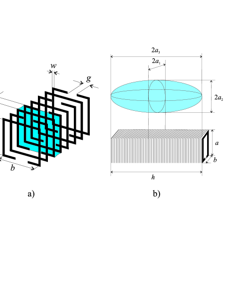
Figure 4: a) A schematic illustration of the metasolenoid. b) A finite-size metasolenoid approximated as a magnetic ellipsoid.

The measured artificial magnetic particle, metasolenoid, is schematically presented in Fig. 4a. In [8] the effective permeability of a medium densely filled with infinitely long metasolenoids was derived in the form

$$\mu_{\rm eff}=1-V_{\rm r}\frac{j\omega\mu_{0}S}{Z_{\rm tot}d},$$ (17)

where $V_{\rm r}$ is the volume filling ratio, $S=a\times b$ is the cross section are of the ring, $d$ is the distance between the rings, and the total effective impedance was presented in the form

$$Z_{\rm tot}=j\omega{L_{\rm eff}}+\frac{1}{j\omega C_{\rm eff}}+R_{\rm eff}.$$ (18)

For the experimental validation a finite-size metasolenoid was approximated as an ellipsoid cut off from a magnetic media described by (17), Fig. 4b. The magnetic polarizability of the ellipsoid $\alpha_{\rm mm}$ was analytically calculated using the classical mixing theory [25]. The scattering amplitude of an electrically small material sample was measured using a standard parallel plate waveguide, and the theory of waveguide excitation was used to calculate the magnetic polarizability from the measured results. It is worth noting that the magnetic polarizability is a function of the magnetic permeability due to the mixing process. On the other hand, permeability is defined using the equivalent circuit, Fig. 3b. Thus, the magnetic polarizablity of the measured sample contains all the relevant data for validating both the proposed equivalent circuit and the permeability function.

Though it is not explicitly mentioned in [8], substrate losses were taken into account when analytically calculating the magnetic polarizability of the sample. The authors used (18) to define the total impedance of the metasolenoid unit cell, however, complex permittivity was used when calculating the effective capacitance. Thus, the equivalent circuit of the unit cell used to analyze the measured sample is the proposed circuit shown in Fig. 3b. It can easily be verified using the data presented in [8] that the following expression for the effective impedance (derived using the circuit in Fig. 3b) exactly repeats the analytical estimation for the magnetic polarizability of the sample:

$$Z_{\rm tot}^{\prime}=j\omega L_{\rm eff}+R_{\rm eff}+\frac{R_{\rm d}}{1+j\omega C_{\rm eff}R_{\rm d}},$$ (19)

where $R_{\rm d}=\epsilon^{\prime}/(\epsilon^{\prime\prime}\omega C_{\rm eff})$. The analytically calculated [$Z_{\rm tot}$ given by (19) is used in (17)] and measured magnetic polarizabilities are shown in Fig. 5. The measured and calculated key parameters are gathered in Table I. The polarizability and permeability values in Table I are the maximum values.

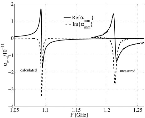
Figure 5: The analytically calculated (proposed model) and measured magnetic polarizability.

The measured results agree rather closely with the analytical calculations when the proposed model is used. The slight difference in the resonant frequencies, and the slightly lowered polarizability values in the measurement case are most likely caused by limitations in the accuracy of the manufacturing process: The implemented separation between the rings is probably slightly larger than the design value. This lowers the effective capacitance and is seen as a weakened magnetic response and the higher resonant frequency. Moreover, the measured Im$\{\alpha_{\rm mm}\}$ clearly indicates that the effect of the lossy glue used to stack the rings is underestimated in the analytical calculations. In the analytical calculations $\tan\delta=0.002$ was used for the total loss tangent [8]. A loss tangent value $\tan\delta=0.0025$ would accurately produce the measured polarizability values, and the bandwidths (defined from the Im$\{\alpha_{\rm mm}\}$ curve) would visually coincide.

If the matrix losses are neglected in the circuit model [$R_{\rm d}\rightarrow\infty$ in (19)], the analytical calculations lead to dramatically overestimated polarizability and permeability values. It is therefore evident that the proposed generalization of the circuit model and the permeability function have a significant practical importance. Though the model has been validated using a specific example, we can conclude that matrix losses can strongly dominate over conductive losses in structures where the unit cells are closely spaced. This is physically well understandable since in this case most of the flux is forced inside the substrate.

TABLE I: Analytically calculated and measured properties of the metasolenoid sample.

	$F_{\rm res}$	Re$\{\alpha_{\rm mm}\}$	$|\alpha_{\rm mm}|$	Re$\{\mu_{\rm eff}\}$
	GHz	H$\cdot$m2	H$\cdot$m2
Analytical†	1.09	1.7$\times 10^{-11}$	3.3$\times 10^{-11}$	230
Measured	1.21	1.4$\times 10^{-11}$	2.7$\times 10^{-11}$	—
Analytical‡	1.09	19.9$\times 10^{-11}$	60.1$\times 10^{-11}$	4000

^†proposed model, ^‡old model

VI Electromagnetic field energy density

Following the approach introduced in [20] we will next generalize the expression for the energy density in artificial magnetics using the experimentally validated circuit model. In the time-harmonic regime the total stored energy reads (notations are clear from Fig. 3b)

$$W=\frac{1}{2}(L_{0}|I|^{2}+L|I_{\rm L}|^{2}+C|V_{\rm C}|^{2})$$

$$=\frac{1}{2}\bigg{[}L_{0}|I|^{2}+|I_{\rm L}|^{2}\bigg{(}L+\frac{1}{C(\omega^{2}+\frac{1}{C^{2}R_{\rm d}^{2}})}\bigg{)}\bigg{]},$$ (20)

$$|I_{\rm L}|^{2}=\frac{\omega^{2}\frac{M^{2}}{L^{2}}\bigg{(}\omega^{2}+\frac{1}{C^{2}R_{\rm d}^{2}}\bigg{)}}{[(1+\frac{R}{R_{\rm d}})\frac{1}{LC}-\omega^{2}]^{2}+\omega^{2}{(\frac{R}{L}+\frac{1}{CR_{\rm d}})^{2}}}|I|^{2}.$$ (21)

Using the notations in (11) the stored energy can be written as

$$W=\frac{1}{2}L_{0}|I|^{2}\bigg{(}1+\frac{A\omega^{2}(\omega_{\rm 0}^{2}+\omega^{2}+\Gamma_{\rm d}^{2})}{(\widetilde{\omega}_{\rm 0}^{2}-\omega^{2})^{2}+\omega^{2}(\Gamma+\Gamma_{\rm d})^{2}}\bigg{)}.$$ (22)

The inductance per unit length of a tightly wound long solenoid is $L_{0}=\mu_{0}n^{2}S$, where $n$ is the number of turns per unit length and $S$ is the cross section area. The relation between the current $I$ and magnetic field $H$ inside the solenoid is $I=H/n$. Thus, the stored energy in one unit-length section of the solenoid reads

$$W=w_{\rm m}S=\frac{1}{2}\mu_{0}n^{2}S\frac{|H|^{2}}{n^{2}}\bigg{(}1+\frac{A\omega^{2}(\omega_{\rm 0}^{2}+\omega^{2}+\Gamma_{\rm d}^{2})}{(\widetilde{\omega}_{\rm 0}^{2}-\omega^{2})^{2}+\omega^{2}(\Gamma+\Gamma_{\rm d})^{2}}\bigg{)},$$ (23)

from which we identify the expression for the electromagnetic field energy density in the artificial material sample:

$$w_{\rm m}=\frac{\mu_{0}}{2}\bigg{(}1+\frac{A\omega^{2}(\omega_{\rm 0}^{2}+\omega^{2}+\Gamma_{\rm d}^{2})}{(\widetilde{\omega}_{\rm 0}^{2}-\omega^{2})^{2}+\omega^{2}(\Gamma+\Gamma_{\rm d})^{2}}\bigg{)}|H|^{2}.$$ (24)

We immediately note that if there is no loss in the matrix material ($R_{\rm d}\rightarrow\infty$ and $\Gamma_{\rm d}\rightarrow 0$), then $\widetilde{\omega}_{\rm p}^{2}\rightarrow\omega_{\rm p}$ and (24) reduces to (6).

VI-A Comparison with the results obtained using the ED-method

The above derived result differs from the result found in [21] using the ED-method:

$$w_{\rm m}=\frac{\mu_{0}}{2}\bigg{(}1+\frac{A\omega^{2}[\omega_{\rm 0}^{2}(3\omega_{0}^{2}-\omega^{2})+\omega^{2}\Gamma^{2}]}{\omega_{\rm 0}^{2}[(\omega_{0}^{2}-\omega^{2})^{2}+\omega^{2}\Gamma^{2}]}\bigg{)}|H|^{2}.$$ (25)

The procedure and the underlying assumptions to obtain (25) have been briefly revised in Section II. The classical expression for the magnetic field energy density in a media where absorption due to losses can be neglected reads [22, 23]

$$w_{\rm m}=\frac{\mu_{0}}{2}\frac{\partial(\omega\mu_{\rm r}(\omega))}{\partial\omega}|H|^{2}.$$ (26)

It is seen that in the presence of negligible losses [$\Gamma\rightarrow 0$ in (1)] the energy density result given by (25) is the same as the result predicted by the classical expression (26). However, (24) predicts a different result. Authors of [21] use this fact to state that the result obtained using the ED-method is more internally consistent than the result obtained using the EC-method.

The EC-method is known to give a perfectly internally consistent result for the energy density in dielectrics obeying the general Lorentzian type dispersion law [20]. The general Lorentz model is a strictly causal model. This is, however, not the case with the modified Lorentz model (1). As is speculated already in [20], the reason for the difference in the results obtained using (24) and (26) in the small-loss limit is related to the physical limitations of the quasi-static permeability model (1). Thus, when (1) is used as the macroscopic media description, (24) should be used also in the presence of vanishingly small losses. The ED-method, though being internally consistent with the classical expression, predicts unphysical behavior at high frequencies: At high frequencies the energy density given by the ED-method is smaller than the energy density in vacuum (when there are no losses, this unphysical behavior takes place at frequencies $\omega>\sqrt{3}\omega_{\rm 0}$, where restriction (2) is violated), Fig. 1a and 1b in [21]. This behavior is avoided with the result obtained using the EC-method, since that approach is based on the microscopic description of the medium, which is always in harmony with the causality principle.

Fig. 6 depicts the normalized magnetic field energy density in a medium formed by the metasolenoids introduced in the previous section. The amplitude factor $A=1$, and the loss factors have been estimated using (11) and the data presented in [8]. In this particular example the energy densities given by (24) and (6) give practically the same result over the whole studied frequency range (the result given by (6) is not plotted in Fig. 6 since the result visually coincides with the EC-result). This is due to the fact that large values of $\omega$ and $\omega_{\rm 0}$ mask the effect of $\Gamma$ and $\Gamma_{\rm d}$ in (24) and (6). The results given by the ED-method and the classical expression (26) also visually coincide. However, as was mentioned above, the energy density expression given by the ED-method predicts the same nonphysical behavior as the classical expression: The field energy density is smaller than the energy density in vacuum at frequencies $\omega>\sqrt{3}\omega_{\rm 0}$.

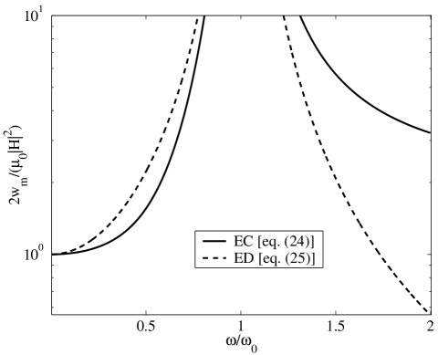
Figure 6: Magnetic field energy density given by different expressions. $\omega_{0}$ is the resonant frequency of the metasolenoid medium.

Conclusion

In this paper we have explained differences between recent approaches used to derive field energy density expressions for artificial magnetic media. The equivalent circuit model of split-ring resonators and other similar structures has been generalized to take account losses in the dielectric matrix material. It has been shown that a modification is needed to the macroscopic permeability function commonly used to model these materials in the quasi-static regime. Moreover, depending on the nature of the dominating loss mechanism in the matrix material, the permeability function has different forms. The proposed circuit model and the modified permeability function have been experimentally validated, and it has been shown that in a practical situation matrix losses can dramatically dominate over conductive losses. Using the validated circuit model we have derived an expression for the electromagnetic field energy density in artificial magnetic media. This expression is valid also when losses in the material cannot be neglected and when the medium is strongly dispersive. The results have been compared to the recently reported results.

References

- [1] M. V. Kostin and V. V. Shevchenko, “Artificial magnetics based on double circular elements,” Proc. Bianisotropics’94, Périgueux, France, pp. 49–56, May 18–20, 1994.
- [2] J. B. Pendry, A. J. Holden, D. J. Robbins, W. J. Stewart, “Magnetism from conductors and enhanced nonlinear phenomena,” IEEE Trans. Microwave Theory Tech., vol. 47, no. 11, pp. 2075–2084, Nov. 1999.
- [3] R. Marqués, F. Medina, R. Rafii-El-Idrissi, “Role of bianisotropy in negative permeability and left-handed metamaterials,” Phys. Rev. B, vol. 65, 1444401(–6), April 2002.
- [4] M. Gorkunov, M. Lapine, E. Shamonina, K. H. Ringhofer, “Effective magnetic properties of a composite material with circular conductive elements”, European Phys. Journal B, vol. 28, no. 3, pp. 263–269, July 2002.
- [5] A. N. Lagarkov, V. N. Semenenko, V. N. Kisel, V. A. Chistyaev, “Development and simulation of microwave artificial magnetic composites utilizing nonmagnetic inclusions,” J. Magnetism and Magnetic Materials, vol. 258–259, pp. 161–166, March 2003.
- [6] B. Sauviac, C. R. Simovski, S. A. Tretyakov, “Double split-ring resonators: Analytical modeling and numerical simulations,” Electromagnetics, vol. 24, no. 5, pp. 317–338, 2004.
- [7] J. D. Baena, R. Marqués, F. Medina, J. Martel, “Artificial magnetic metamaterial design by using spiral resonators,” Phys. Rev. B, 69, 014402, Jan. 2004.
- [8] S. I. Maslovski, P. Ikonen, I. A. Kolmakov, S. A. Tretyakov, M. Kaunisto, “Artificial magnetic materials based on the new magnetic particle: Metasolenoid,” Progress in Electromagnetics Research, vol. 54, pp. 61–81, 2005.
- [9] D. R. Smith, W. J. Padilla, D. C. Vier, S. C. Nemat-Nasser, S. Schultz, “Composite medium with simultaneously negative permeability and permittivity,” Phys. Rev. Lett., vol. 84, no. 18, pp. 4184–4187, May 2000.
- [10] R. A. Shelby, D. R. Smith, S. Schultz, “Experimental verification of a negative index of refraction,” Science, vol. 292, pp. 77–79, April 2001.
- [11] R. C. Hansen and M. Burke, “Antenna with magneto-dielectrics,” Microwave Opt. Technol. Lett., vol. 26, no. 2., pp. 75–78, July 2000.
- [12] S. Yoon and R. W. Ziolkowski, “Bandwidth of a microstrip patch antenna on a magneto-dielectric substrate,” IEEE Antennas Propagat. Soc. Int. Symposium, Columbus, Ohio, pp. 297–300, June 22-27, 2003.
- [13] H. Mossallaei and K. Sarabandi “Magneto-dielectrics in electromagnetics: Concept and applications,” IEEE Trans. Antennas Propagat., vol. 52, no. 6, pp. 1558–1567, June 2004.
- [14] M. K. Kärkkäinen, S. A. Tretyakov, P. Ikonen, “PIFA with dispersive material fillings,” Microwave Opt. Technol. Lett., vol. 45, no. 1, pp. 5–8, April 2005.
- [15] M. E. Ermutlu, C. R. Simovski, M. K. Kärkkäinen, P. Ikonen, S. A. Tretyakov, A. A. Sochava, “Miniaturization of patch antennas with new artificial magnetic layers,” 2005 IEEE Int. Workshop on Antenna Technology, Singapore, pp. 87–90, March 7–9, 2005.
- [16] K. Buell, H. Mosallaei, K. Sarabandi, “A substrate for small patch antennas providing tunable miniaturization factors,” IEEE Trans. Microwave Theory Tech., vol. 54, no. 1., pp. 135–145, Jan. 2006.
- [17] P. Ikonen, S. Maslovski, C. Simovski, S. Tretyakov, “On artificial magneto-dielectric loading for improving the impedance bandwidth properties of microstrip antennas,” arXiv:physics/0509139. (To appear in IEEE Trans. Antennas Propagat., June 2006.)
- [18] R. Ruppin, “Electromagnetic energy density in a dispersive and absorptive material,” Phys. Lett. A, vol. 299, pp. 309–312, July 2002.
- [19] T. J. Cui and J. A. Kong, “Time-domain electromagnetic energy in a frequency-dispersive left-handed medium,” Phys. Rev. B, vol. 70, 205106, Nov. 2004.
- [20] S. A. Tretyakov, “Electromagnetic field energy density in artificial microwave materials with strong dispersion and loss,” Phys. Lett. A, vol. 343, pp. 231–237, June 2005.
- [21] A. D. Boardman and K. Marinov, “Electromagnetic energy in a dispersive metamaterial,” Phys. Rev. B, vol. 73, 165110, April 2006.
- [22] L. D. Landau, E. M. Lifshits, Electrodynamics of continuous media, 2nd ed., Pergamon: Oxford, England, 1984.
- [23] L. A. Vainstein, Electromagnetic waves, 2nd ed., Radio i Sviaz: Moscow, 1988 (in Russian).
- [24] J. D. Jackson, Classical electrodynamics, 3rd ed., John Wiley Sons: New York, 1999.
- [25] A. Sihvola, Electromagnetic mixing rules and formulas, IEE Electromagnetic Waves Series: London, 1999.