Efficient computation of matched solutions of the Kapchinskij-Vladimirskij envelope equations for periodic focusing lattices

Abstract

A new iterative method is developed to numerically calculate the periodic, matched beam envelope solution of the coupled Kapchinskij-Vladimirskij (KV) equations describing the transverse evolution of a beam in a periodic, linear focusing lattice of arbitrary complexity. Implementation of the method is straightforward. It is highly convergent and can be applied to all usual parameterizations of the matched envelope solutions. The method is applicable to all classes of linear focusing lattices without skew couplings, and also applies to all physically achievable system parameters – including where the matched beam envelope is strongly unstable. Example applications are presented for periodic solenoidal and quadrupole focusing lattices. Convergence properties are summarized over a wide range of system parameters.

I INTRODUCTION

The Kapchinskij-Vladimirskij (KV) envelope equationsKapchinskij and Vladimirskij (1959); Reiser (1994); Lund and Bukh (2004) are often employed as a simple description of the transverse evolution of intense ion beams. The equations are coupled ordinary differential equations that describe the evolution of the beam edge (or rms radii) in response to applied linear focusing forces of the lattice and defocusing forces resulting from beam space-charge and transverse phase-space area (emittances). Although the KV envelope equations are only fully Vlasov consistent with the singular KV distribution, the equations can be applied to describe the low-order evolution of a real distribution of beam particles when the variation of the statistical beam emittances is negligible or sufficiently slowReiser (1994). Large nonlinear fields that can be produced by non-ideal applied focusing elements, nonuniform beam space-charge, and species contamination (electron cloud effects, etc.) drive deviations from the KV model. Such effects are suppressed to the extent possible in most practical designs, rendering the KV model widely applicable.

The matched solution of the KV envelope equations is the solution with the same periodicity as the focusing latticeKapchinskij and Vladimirskij (1959); Reiser (1994); Lund and Bukh (2004). The matched beam envelope is important because it is believed to be the most radially compact solution supported by a periodic linear focusing channelLund and Bukh (2004). Matched envelopes are typically calculated as a first step in the design of practical transport lattices and for use in initializing more detailed beam simulations to evaluate machine performanceReiser (1994). The matched envelope solution is typically calculated by numerically integrating trial solutions of the KV equations from assumed initial conditions over one lattice period and searching for the four initial envelope coordinates and angles that generate the solution with the periodicity of the latticeReiser (1994); Ryne (1995); Lund and Bukh (2004). An optimal formulation of the conventional root finding procedure for envelope matching has been presented by RyneRyne (1995). Conventional root finding procedures for matching can be surprisingly problematic even for relatively simple focusing lattices. Variations in initial conditions can lead to many inflection points in the envelope functions at the end of the lattice period. Thus initial guesses close to the actual values corresponding to the periodic solution are often necessary to employ standard root finding techniques. This is especially true for complicated focusing lattices with low degrees of symmetry and where focusing strengths (or equivalently, undepressed single particle phase advances) are large. For large focusing strength and strong space-charge intensity, the matched envelope solution can be unstable over a wide range of system parametersReiser (1994); Lund and Bukh (2004). Such instabilities can restrict the basin of attraction when standard numerical root finding methods are used to calculate the needed matching conditions — especially for certain classes of solution parameterizations.

In this article we present a new iterative procedure to numerically calculate matched envelope solutions of the KV equations. The basis of this procedure is that the KV distribution of particle orbits internal to the beam must have a locus of turning points consistent with the beam edge (envelope). In the absence of beam space-charge, betatron amplitudes calculated from the sine- and cosine-like principal orbits describing particles moving in the applied focusing fields of the lattice directly specify the matched beam envelopeWiedemann (1993). For finite beam space-charge, the principal orbits describing the betatron amplitudes and matched beam envelope cannot be a priori calculated because the defocusing forces from beam space-charge uniformly distributed within the (undetermined) beam envelope are unknown. In the iterative matching (IM) method, the relation between the betatron amplitudes and the particle orbits is viewed as a consistency equation. Starting from a simple trial envelope solution that accounts for both space-charge and and applied focusing forces in a general manner, the consistency condition is used to iteratively correct the envelope functions until converged matched envelope solutions are obtained that are consistent with particle orbits internal to the beam.

The IM method offers superior performance and reliability in constructing matched envelopes over conventional root finding because the IM iterations are structured to reflect the periodicity of the actual matched solution rather than searching for parameters that lead to periodicity. The IM method works for all physically achievable system parameters (even in cases of envelope instability) and is most naturally expressed and rapidly convergent when relative beam space-charge strength is expressed in terms of the depressed particle phase advance. All other parameterizations of solutions (specified perveances and emittances, etc.) can also be carried out by simple extensions of the IM method rendering the approach fully general. The natural depressed phase advance parameterization is also useful when carrying out parametric studies because phase advances are the most relevant parameters for analysis of resonance-like effects central to charged particle dynamics in accelerators. The IM method provides a complement to recent analytical perturbation theories developed to construct matched beam envelopes in lattices with certain classes of symmetriesLee (1996, 2002); Anderson (2005a, b). In contrast to these analytical theories, the IM method can be applied to arbitrary linear focusing lattices without skew couplings. The highly convergent iterative corrections of the IM method have the same form for all order iterations after seeding, rendering the method straightforward to code and apply to numerically generate accurate matched envelope solutions.

The organization of this paper is the following. After a review of the KV envelope equations in Sec. II, various properties of matched envelope solutions and the continuous focusing limit are analyzed in Sec. III. These results are used in Sec. IV to formulate the IM method for calculation of matched solutions to the KV envelope equations. Example applications of the IM method are presented in Sec. V to illustrate application and convergence properties of the method over a wide range of system parameters for a variety of systems. Concluding comments in Sec VI summarize the advantages of the IM method over conventional techniques.

II THEORETICAL MODEL

We consider an unbunched beam of particles of charge $q$ and mass $m$ coasting with axial relativistic factors $\beta_{b}=\text{const}$ and $\gamma_{b}=1/\sqrt{1-\beta_{b}^{2}}$. In the KV model, the beam is propagating in a linear focusing lattice without skew couplings and has uniform charge density within an elliptical cross-section with principal radii $r_{x}$ and $r_{y}$ along the (transverse) $x$- and $y$-coordinate axes. When self-fields are included and image effects are neglected, the envelope radii consistent with the KV distribution evolve according to the so-called KV envelope equationsKapchinskij and Vladimirskij (1959); Reiser (1994); Lund and Bukh (2004)

$$r_{j}^{\prime\prime}(s)+\kappa_{j}(s)r_{j}(s)-\frac{2Q}{r_{x}(s)+r_{y}(s)}-\frac{\varepsilon_{j}^{2}}{r_{j}^{3}(s)}=0.$$ (1)

Here, primes denote derivatives with respect to the axial machine coordinate $s$, the subscript $j$ ranges over both transverse coordinates $x$ and $y$, the functions $\kappa_{j}(s)$ represent linear applied focusing forces of the transport lattice, $Q=\text{const}$ is the dimensionless perveance, and $\varepsilon_{j}=\text{const}$ are the rms edge emittances. Equations relating the functions $\kappa_{j}$ to magnetic and/or electric fields of practical focusing elements are presented in Ref. Lund and Bukh (2004). The perveance provides a dimensionless measure of self-field defocusing forces internal to the beamReiser (1994) and is defined as

$$Q=\frac{qI}{2\pi\epsilon_{0}mc^{3}\gamma_{b}^{3}\beta_{b}^{3}}.$$ (2)

Here, $I$ is the constant beam current, $c$ is the speed of light in vacuo, and $\epsilon_{0}$ is the permittivity of free space. The perveance $Q$ can be thought of as a scaled measure of space-charge strengthReiser (1994). The rms edge emittances $\varepsilon_{j}$ provide a statistical measure of beam phase-space area projections in the $x$–$x^{\prime}$ and $y$–$y^{\prime}$ planesReiser (1994).

When the emittances are constant ($\varepsilon_{j}=\text{const}$), the KV envelope equations (1) are consistent with the Vlasov equation only for the KV distributionKapchinskij and Vladimirskij (1959); Davidson (1990), which is a singular function of Courant-Snyder invariants. This singular structure can lead to unphysical instabilities within the Vlasov modelHofmann et al. (1983). However, the KV envelope equations can be applied to physical (smooth) distributions in an rms equivalent beam senseReiser (1994), with the envelope radii and the emittances defined by statistical averages of the physical distribution as

$$r_{x}=2\sqrt{\langle x^{2}\rangle},\hskip 28.45274ptr_{y}=2\sqrt{\langle y^{2}\rangle},$$ (3)

and

$$\varepsilon_{x} =4\left[\langle x^{2}\rangle\langle x^{\prime 2}\rangle-\langle xx^{\prime}\rangle^{2}\right]^{1/2},$$ (4)

$$\varepsilon_{y} =4\left[\langle y^{2}\rangle\langle y^{\prime 2}\rangle-\langle yy^{\prime}\rangle^{2}\right]^{1/2}.$$

Here, $\langle\cdots\rangle$ denotes a transverse statistical average over the beam distribution function, and for notational simplicity, we have assumed zero centroid offset (e.g., $\langle x\rangle=0$). In this rms equivalent sense, the emittances $\varepsilon_{j}$ will generally evolve in $s$. If this variation has negligible effect on the $r_{j}$, then the KV envelope equations can be applied with $\varepsilon_{j}=\text{const}$ to reliably model practical machines. This must generally be verified a posteriori with simulations of the full distribution.

For appropriate choices of the lattice focusing functions $\kappa_{j}(s)$, Eq. (1) can be employed to model a wide range of transport channels, including solenoidal and quadrupole transport. For solenoidal transport, the equations must be interpreted in a rotating Larmor frame (see Appendix A of Ref. Lund and Bukh (2004)). In a periodic transport lattice, the $\kappa_{j}$ are periodic with fundamental lattice period $L_{p}$, i.e.,

$$\kappa_{j}(s+L_{p})=\kappa_{j}(s).$$ (5)

The beam envelope is said to be matched to the transport lattice when the envelope functions have the same periodicity as the lattice:

$$r_{j}(s+L_{p})=r_{j}(s).$$ (6)

For specified focusing functions $\kappa_{j}(s)$, beam perveance $Q$, and emittances $\varepsilon_{j}$, the matching condition is equivalent to requiring that $r_{j}$ and $r_{j}^{\prime}$ satisfy specific initial conditions at $s=s_{i}$ when the envelope equations (1) are integrated as an initial value problem. The required initial conditions generally vary with the phase of $s_{i}$ in the lattice period (because the conditions vary with the local matched solution). In conventional procedures for envelope matching, needed initial conditions are typically found by numerical root finding starting from guessed seed valuesLund and Bukh (2004). This numerical matching can be especially problematic when: applied focusing strengths are large, the focusing lattice is complicated and devoid of symmetries that can reduce the dimensionality of the root finding, choices of solution parameters require extra constraints to effect, and where the matched beam envelope is unstable.

The undepressed particle phase advance per lattice period $\sigma_{0j}$ provides a dimensionless measure of the strength of the applied focusing functions $\kappa_{j}$ describing the periodic latticeWiedemann (1993); Lund and Bukh (2004). The $\sigma_{0j}$ can be calculated fromWiedemann (1993)

$$\cos\sigma_{0j}=\frac{1}{2}{\rm Tr}\;{\bf M}_{0j}(s_{i}+L_{p}|s_{i}),$$ (7)

where ${\bf M}_{0j}(s|s_{i})$ denotes the $2\times 2$ single particle transfer matrix in the $j$-plane from axial coordinate $s_{i}$ to $s$. Explicitly, we have

$${\bf M}_{0j}(s|s_{i})=\left(\begin{array}[]{ll}C_{0j}(s|s_{i})&S_{0j}(s|s_{i})\\ C_{0j}^{\prime}(s|s_{i})&S_{0j}^{\prime}(s|s_{i})\end{array}\right),$$ (8)

where the $C_{0j}(s|s_{i})$ and $S_{0j}(s|s_{i})$ denote cosine-like and sine-like principal orbit functions satisfying

$$F_{0j}^{\prime\prime}(s|s_{i})+\kappa_{j}(s)F_{0j}(s|s_{i})=0,$$ (9)

with $F$ representing $C$ or $S$ with $C_{0j}$ subject to cosine-like initial ($s=s_{i}$) conditions $C_{0j}(s_{i}|s_{i})=1$ and $C_{0j}^{\prime}(s_{i}|s_{i})=0$, and with $S_{0j}$ subject to sine-like initial conditions $S_{0j}(s_{i}|s_{i})=0$ and $S_{0j}^{\prime}(s_{i}|s_{i})=1$. Equation (7) can be expressed in terms of $C_{0j}$ and $S_{0j}^{\prime}$ as

$$\cos\sigma_{0j}=\frac{1}{2}[C_{0j}(s_{i}+L_{p}|s_{i})+S_{0j}^{\prime}(s_{i}+L_{p}|s_{i})].$$ (10)

The $\sigma_{0j}$ are independent of the particular value of $s_{i}$ used in the calculation of the principal functions. For some particular cases such as piecewise constant $\kappa_{j}$ the principal functions $F_{0j}$ can be calculated analytically. But, in general, the $F_{0j}$ must be calculated numerically. In the absence of space-charge, the particle orbit is stable whenever $\sigma_{0j}<180^{\circ}$ and parametric bands of stability can also usually be found for $\sigma_{0j}>180^{\circ}$Courant and Snyder (1958); Reiser (1994); Lund and Bukh (2004). For a stable orbit, the scale of the $\kappa_{j}$ (i.e., $\kappa_{j}\rightarrow\alpha\kappa_{j}$ with $\alpha=\text{const}$ setting the scale of the specified $\kappa_{j}$) can always be regarded as being set by the $\sigma_{0j}$. In this context, Eq. (10) is employed to fix the scale of the $\kappa_{j}$ in terms of $\sigma_{0j}$ and other parameters defining the $\kappa_{j}$. Because there appears to be no advantage in using stronger focusing with $\sigma_{0j}>180^{\circ}$ in terms of producing more radially compact matched envelopesLund and Bukh (2004); Lee and Briggs (1997), we will assume in all analysis that follows that the $\kappa_{j}$ are sufficiently weak to satisfy $\sigma_{0}<180^{\circ}$.

The formulation given above for calculation of the undepressed principal orbits $C_{0j}$ and $S_{0j}$ and the undepressed particle phase advances $\sigma_{0j}$ can also be applied to calculate the depressed principal orbits $C_{j}$ and $S_{j}$ and the depressed phase advances $\sigma_{j}$ in the presence of uniform beam space-charge density for a particle moving within the matched KV beam envelopes. This is done by replacing

$$\kappa_{j}\rightarrow\kappa_{j}-\frac{2Q}{(r_{x}+r_{y})r_{j}}$$ (11)

in Eqs. (9) and dropping the subscript $0$s in Eqs. (7)–(10) for notational clarity (i.e., $C_{0j}\rightarrow C_{j}$ and $S_{0j}\rightarrow S_{j}$). Explicitly, the depressed principal functions satisfy

$$F_{j}^{\prime\prime}(s|s_{i})+\kappa_{j}(s)F_{j}(s|s_{i})-\frac{2QF_{j}(s|s_{i})}{[r_{x}(s)+r_{y}(s)]r_{j}(s)}=0,$$ (12)

with $F$ representing $C$ or $S$ with $C_{j}$ subject to $C_{j}(s_{i}|s_{i})=1$ and $C_{j}^{\prime}(s_{i}|s_{i})=0$, and $S_{j}$ subject to $S_{j}(s_{i}|s_{i})=0$ and $S_{j}^{\prime}(s_{i}|s_{i})=1$, and the depressed phase advances satisfy

$$\cos\sigma_{j}=\frac{1}{2}[C_{j}(s_{i}+L_{p}|s_{i})+S_{j}^{\prime}(s_{i}+L_{p}|s_{i})].$$ (13)

For a stable orbit, it can be shown that the $\sigma_{j}$ can also be calculated from the matched envelope asWiedemann (1993); Lund and Bukh (2004)

$$\sigma_{j}=\varepsilon_{j}\int_{s_{i}}^{s_{i}+L_{p}}\!\frac{ds}{r_{j}^{2}(s)}.$$ (14)

This formula can also be applied to calculate $\sigma_{0j}$ by using the matched envelope functions $r_{j}$ calculated with $Q=0$.

Matched envelope solutions of Eqs. (1) can be regarded as being determined by the focusing functions $\kappa_{j}$, the perveance $Q$, and the emittances $\varepsilon_{j}$. The lattice period $L_{p}$ is implicitly specified through the $\kappa_{j}$. We will always regard the scale of the $\kappa_{j}$ as being set by the undepressed phase advances $\sigma_{0j}$ through Eq. (10). For $\sigma_{0j}<180^{\circ}$ there is no ambiguity in scale choice and the use of the $\sigma_{0j}$ as parameters allows disparate classes of lattices to be analyzed in a common frameworkLund and Bukh (2004). The depressed phase advances $\sigma_{x}$ and $\sigma_{y}$ can be employed to replace up to two of the three parameters $Q$, $\varepsilon_{x}$, and $\varepsilon_{y}$. Such replacements can be convenient, particularly when carrying out parametric surveys (for example, see Ref. Lund and Bukh (2004)) because $\sigma_{j}/\sigma_{0j}$ is a dimensionless measure of space-charge strength satisfying $0\leq\sigma_{j}/\sigma_{0j}\leq 1$ with $\sigma_{j}/\sigma_{0j}\rightarrow 1$ representing a warm beam with negligible space-charge (i.e., $Q\rightarrow 0$, or $\varepsilon_{j}\rightarrow\infty$ for finite $Q$), and $\sigma_{j}/\sigma_{0j}\rightarrow 0$ representing a cold beam with maximum space-charge intensity (i.e., $\varepsilon_{j}\rightarrow 0$). We will discuss calculation of matched beam envelopes for the useful parameterization cases listed in Table 1. In cases typical of linear accelerators the focusing functions have equal strength in the $x$- and $y$-planes giving $\sigma_{0x}=\sigma_{0y}$. In such plane symmetric cases we denote $\sigma_{0j}\equiv\sigma_{0}$. In practical situations where the focusing lattice and emittances are both plane symmetric with $\sigma_{0j}\equiv\sigma_{0}$ and $\varepsilon_{j}\equiv\varepsilon$, then the depressed phase advance is also plane symmetric with $\sigma_{j}\equiv\sigma$ and parameterization cases $2$ and $3$ are identical. It is assumed that a unique matched envelope solution exists independent of the parameterization when the $\kappa_{j}$ are fully specified. There is no known proof of this conjecture, but numerical evidence suggests that it is correct for simple focusing lattices (i.e., simple $\kappa_{j}$) when $\sigma_{0j}<180^{\circ}$. In typical experimental situations, note that transport lattices are fixed in geometry and excitations of focusing elements in the lattices can be individually adjusted. In the language adopted here, such lattices with different excitations in focusing elements (both overall scale and otherwise) correspond to different lattices described by different $\kappa_{j}$ with corresponding different matched envelopes.

Table 1: Possible parameterizations of matched envelope solutions.

Case	Parameters
$0$	$\kappa_{j}$ ($\sigma_{0j}$), $Q$, $\varepsilon_{j}$
$1$	$\kappa_{j}$ ($\sigma_{0j}$), $Q$, $\sigma_{j}$
$2$	$\kappa_{j}$ ($\sigma_{0j}$), $\varepsilon_{j}$, and one of $\sigma_{j}$
$3$	$\kappa_{j}$ ($\sigma_{0j}$), $\sigma_{j}$, and one of $\varepsilon_{j}$

III MATCHED ENVELOPE PROPERTIES

In development of the IM method in Sec. IV, we employ a consistency equation between depressed particle orbits within the beam and the matched envelope functions (III.1) and use a continuous focusing description of the matched beam (III.2) to construct a seed iteration. Henceforth, we denote lattice period averages with overbars, i.e., for some quantity $\zeta(s)$,

$$\overline{\zeta}\equiv\int_{s_{i}}^{s_{i}+L_{p}}\frac{ds}{L_{p}}\zeta(s).$$ (15)

III.1 Consistency condition between particle orbits and the matched envelope

We calculate nonlinear consistency conditions for the matched envelope functions $r_{j}$ and the depressed principal orbit functions $C_{j}$ and $S_{j}$ as follows. First, the transfer matrix ${\bf M}_{j}$ of the depressed particle orbit in the $j$-plane is expressed in terms of betatron function-like formulation asWiedemann (1993)

$${\bf M}_{j}(s|s_{i})=\left(\begin{array}[]{ll}C_{j}(s|s_{i})&S_{j}(s|s_{i})\\ C_{j}^{\prime}(s|s_{i})&S_{j}^{\prime}(s|s_{i})\end{array}\right)$$ (16)

with,

$$C_{j}(s|s_{i}) =\frac{r_{j}(s)}{r_{j}(s_{i})}\cos\Delta\psi_{j}(s)-\frac{r_{j}^{\prime}(s_{i})r_{j}(s)}{\varepsilon_{j}}\sin\Delta\psi_{j}(s),$$ (17)

$$S_{j}(s|s_{i}) =\frac{r_{j}(s_{i})r_{j}(s)}{\varepsilon_{j}}\sin\Delta\psi_{j}(s),$$

$$C_{j}^{\prime}(s|s_{i}) =\left[\frac{r_{j}^{\prime}(s)}{r_{j}(s_{i})}-\frac{r_{j}^{\prime}(s_{i})}{r_{j}(s)}\right]\cos\Delta\psi_{j}(s)$$

$$-\left[\frac{\varepsilon_{j}}{r_{j}(s_{i})r_{j}(s)}+\frac{r_{j}^{\prime}(s_{i})r_{j}^{\prime}(s)}{\varepsilon_{j}}\right]\sin\Delta\psi_{j}(s),$$

$$S_{j}^{\prime}(s|s_{i}) =\frac{r_{j}(s_{i})}{r_{j}(s)}\cos\Delta\psi_{j}(s)+\frac{r_{j}(s_{i})r_{j}^{\prime}(s)}{\varepsilon_{j}}\sin\Delta\psi_{j}(s).$$

Here,

$$\Delta\psi_{j}(s)=\varepsilon_{j}\int_{s_{i}}^{s}\!\frac{d\tilde{s}}{r_{j}^{2}(\tilde{s})}$$ (18)

is the change in betatron phase of the particle orbit from $s=s_{i}$ to $s$ and the principal functions $C_{j}$ and $S_{j}$ are calculated including the linear space-charge term of the uniform density elliptical beam from Eq. (12) . Note that $r_{j}\equiv\sqrt{\varepsilon_{j}\beta_{j}}$ can be used in Eqs. (17) and (18) to express the results more conventionally in terms of the betatron amplitude functions $\beta_{j}$ describing linear orbits internal to the beam in the $j$-planeWiedemann (1993). These generalized betatron functions are periodic [i.e., $\beta_{j}(s+L_{p})=\beta_{j}(s)$ and include the transverse defocusing effects of uniformly distributed space-charge within the KV equilibrium envelope. Recognizing that $\Delta\psi_{j}(s_{i}+L_{p})=\sigma_{j}$ [see Eq. (14)] and that the matched envelope functions $r_{j}$ have period $L_{p}$ gives

$$\beta_{j}(s)=\frac{r_{j}^{2}(s)}{\varepsilon_{j}}=\frac{[{\bf M}_{j}]_{12}(s+L_{p}|s)}{\sin\sigma_{j}}=\frac{S_{j}(s+L_{p}|s)}{\sin\sigma_{j}}.$$ (19)

Here, $[{\bf M}_{j}]_{12}$ denotes the $1,2$ component of the $2\times 2$ matrix ${\bf M}_{j}$ and $\sigma_{j}$ can be equivalently calculated from either Eq. (13) or Eq. (14).

Equation (19) can be applied to numerically calculate the consistency conditions for the matched envelope functions $r_{j}$ on a discretized axial grid of $s$ locations. As written, the principal orbit functions employed (i.e., the $C_{j}$ and $S_{j}$) need to be independently calculated at each $s$-location on the grid through one lattice period. The fact that every period is the same can be applied to simplify the calculation. For any initial axial coordinate $s_{i}$ we have ${\bf M}_{j}(s+L_{p}|s)={\bf M}_{j}(s+L_{p}|s_{i}+L_{p})\cdot{\bf M}_{j}(s_{i}+L_{p}|s)$. Multiplying this equation from the right side by the identity matrix ${\bf I}={\bf M}_{j}(s|s_{i})\cdot{\bf M}_{j}^{-1}(s|s_{i})$ where ${\bf M}_{j}^{-1}$ is the inverse matrix and using ${\bf M}_{j}(s_{i}+L_{p}|s)\cdot{\bf M}_{j}(s|s_{i})={\bf M}_{j}(s_{i}+L_{p}|s_{i})$ gives

$${\bf M}_{j}(s+L_{p}|s)={\bf M}_{j}(s|s_{i})\cdot{\bf M}_{j}(s_{i}+L_{p}|s_{i})\cdot{\bf M}_{j}^{-1}(s|s_{i}).$$ (20)

Some straightforward algebra employing Eqs. (16), (19), and (20), and the Wronskian (or symplectic) condition on ${\bf M}_{j}$Wiedemann (1993)

$$C_{j}(s|s_{i})S_{j}^{\prime}(s|s_{i})-S_{j}(s|s_{i})C_{j}^{\prime}(s|s_{i})=1$$ (21)

yields

$$\beta_{j}(s)=\frac{r_{j}^{2}(s)}{\varepsilon_{j}}= \frac{S_{j}^{2}(s|s_{i})}{S_{j}(s_{i}+L_{p}|s_{i})/\sin\sigma_{j}}$$ (22)

$$+\frac{S_{j}(s_{i}+L_{p}|s_{i})}{\sin\sigma_{j}}\left[C_{j}(s|s_{i})+\frac{\cos\sigma_{j}-C_{j}(s_{i}+L_{p}|s_{i})}{S_{j}(s_{i}+L_{p}|s_{i})}S_{j}(s|s_{i})\right]^{2}.$$

Equation (22) explicitly shows that the linear principal functions $C_{j}$ and $S_{j}$ need only be calculated in $s$ from some arbitrary initial point ($s_{i}$) over one lattice period (to $s_{i}+L_{p}$) to calculate the consistency condition for the matched envelope functions $r_{j}(s)$, or equivalently, the betatron amplitude functions $\beta_{j}(s)\equiv r_{j}^{2}(s)/\varepsilon_{j}$. Equation (22) can also be derived using Courant-Snyder invariants of particle orbits within the beam.

Equations (13) and (22) form the foundation of an iterative numerical method developed in Sec. IV to calculate the matched beam envelope for any lattice. These equations express the intricate connection between the bundle of depressed particle orbits within the uniform density KV beam and the locus of maximum particle excursions defining the envelope functions $r_{j}$. The method will be iterative because the consistent matched envelope functions $r_{j}$ are necessary to integrate the linear differential equations for the depressed orbit principal functions $C_{j}$ and $S_{j}$. However, in the limit $Q\rightarrow 0$, the principal functions do not depend on the $r_{j}$ and the matched envelope can be immediately calculated from the equations. Thus, the periodic zero-current matched beam envelope can be directly calculated using Eq. (22) in terms of the two independent, aperiodic linear orbits (i.e., $C_{0j}$ and $S_{0j}$) integrated over one lattice period.

Additional constraints on the matched envelope functions $r_{j}$ and/or betatron functions $\beta_{j}$ are necessary to formulate the IM method for parameterizations where one or more of the parameters $Q$ and $\varepsilon_{j}$ need to be eliminated (see Table 1). Appropriate constraints can be derived by taking the period average of Eq. (1) for a matched envelope, giving

$$\overline{\kappa_{j}r_{j}}-2Q\overline{\frac{1}{r_{x}+r_{y}}}-\varepsilon_{j}^{2}\overline{\frac{1}{r_{j}^{3}}}=0.$$ (23)

III.2 Continuous limit

In the continuous focusing approximation, we take the lattice focusing functions $\kappa_{j}$ as constants set according to

$$\kappa_{j}\rightarrow\left(\frac{\sigma_{0j}}{L_{p}}\right)^{2}$$ (24)

with the $\sigma_{0j}$ calculated from Eq. (10) consistent with the actual $s$-varying periodic focusing functions $\kappa_{j}$. Then we replace $r_{j}\rightarrow\overline{r_{j}}$ in the KV envelope equations (1) and take $\overline{r_{j}}=\text{const}$ to obtain the continuous limit envelope equation

$$\left(\frac{\sigma_{0j}}{L_{p}}\right)^{2}\overline{r_{j}}-\frac{2Q}{\overline{r_{x}}+\overline{r_{y}}}-\frac{\varepsilon_{j}^{2}}{\overline{r_{j}}^{3}}=0.$$ (25)

Equation (25) provides an estimate of the lattice period average envelope radii $\overline{r_{j}}$ in response to applied focusing forces and defocusing forces from beam space-charge and thermal (emittance) effects. Solutions for $\overline{r_{j}}$ will be employed to seed the IM method of constructing matched envelope solutions. In general, the continuous limit approximations tend to be more accurate for weaker applied focusing strengths with $\sigma_{0j}\lesssim 80^{\circ}$. However, even for higher values of $\sigma_{0j}<180^{\circ}$, the formulas can still be applied to seed iterative numerical matching methods if the methods have a sufficiently large “basin of attraction” to the desired solution.

For case $0$ parameterizations (specified $\sigma_{0j}$, $Q$, and $\varepsilon_{j}$) the solutions of Eq. (25) will, in general, need to be calculated numerically from a trial guess. Certain limits are analytically accessible and often relevant. If the beam perveance $Q$ is zero, or equivalently if $\sigma_{j}=\sigma_{0j}$, then Eqs. (25) decouple and are trivially solved as

$$\overline{r_{j}}=\sqrt{\frac{\varepsilon_{j}}{(\sigma_{0j}/L_{p})}}.$$ (26)

Alternatively, this result can be obtained using $r_{j}=\overline{r_{j}}$ in Eq. (14) with $\sigma_{j}\rightarrow\sigma_{0j}$. In the case of a symmetric system with $\sigma_{0x}=\sigma_{0y}\equiv\sigma_{0}$ and $\varepsilon_{x}=\varepsilon_{y}\equiv\varepsilon$, then $\overline{r_{x}}=\overline{r_{y}}\equiv\overline{r_{b}}$ and the envelope equations decouple and the resulting quadratic equation in $r_{b}^{2}$ is solved as

$$\overline{r_{b}}=\frac{1}{(\sigma_{0}/L_{p})}\left[\frac{Q}{2}+\frac{1}{2}\sqrt{Q^{2}+4\left(\frac{\sigma_{0}}{L_{p}}\right)^{2}\varepsilon^{2}}\right]^{1/2}.$$ (27)

In parameterization cases $1$–$3$, the continuous limit solutions $\overline{r_{j}}$ must be expressed using the depressed phase advances $\sigma_{j}$ to eliminate one or more of the parameters $Q$ and $\varepsilon_{j}$. In these cases, if the emittances $\varepsilon_{j}$ are known, then Eq. (14) can be employed to estimate

$$\overline{r_{j}}=\sqrt{\frac{\varepsilon_{j}}{(\sigma_{j}/L_{p})}}.$$ (28)

Alternatively, if the perveance $Q$ is known but one or more of the emittances $\varepsilon_{j}$ is unknown, we can use Eq. (28) to eliminate the emittance term(s) in Eq. (25) obtaining $(\sigma_{0j}^{2}-\sigma_{j}^{2})\overline{r_{j}}=2QL_{p}^{2}/(\overline{r_{x}}+\overline{r_{y}})$. Taking the ratio of the $x$- and $y$-equations yields

$$\frac{\overline{r_{y}}}{\overline{r_{x}}}=\frac{\sigma_{0x}^{2}-\sigma_{x}^{2}}{\sigma_{0y}^{2}-\sigma_{y}^{2}}.$$ (29)

Back-substitution of this result in $(\sigma_{0j}^{2}-\sigma_{j}^{2})\overline{r_{j}}=2QL_{p}^{2}/(\overline{r_{x}}+\overline{r_{y}})$ then gives

$$\overline{r_{x}} =\frac{\sqrt{2Q}L_{p}}{\sqrt{(\sigma_{0x}^{2}-\sigma_{x}^{2})+\frac{(\sigma_{0x}^{2}-\sigma_{x}^{2})^{2}}{(\sigma_{0y}^{2}-\sigma_{y}^{2})}}},$$ (30)

$$\overline{r_{y}} =\frac{\sqrt{2Q}L_{p}}{\sqrt{(\sigma_{0y}^{2}-\sigma_{y}^{2})+\frac{(\sigma_{0y}^{2}-\sigma_{y}^{2})^{2}}{(\sigma_{0x}^{2}-\sigma_{x}^{2})}}}.$$

Alternative smooth-limit formulations in the literatureDavidson and Qian (1994); Davidson and Qin (2001) can also be employed to estimate the $\overline{r_{j}}$ for systems with high degrees of symmetry.

IV NUMERICAL ITERATIVE METHOD FOR MATCHED ENVELOPE CALCULATION

We formulate a numerical iterative matching (IM) method to construct the matched beam envelope functions $r_{j}(s)$ over one lattice period $L_{p}$ using the developments in Sec. III. The IM method is formulated for arbitrary periodic focusing functions $\kappa_{j}$. Constraints necessary to apply the IM formalism to all cases of envelope parameterizations listed in Table 1 are derived.

Label all quantities varying with iteration number with a superscript $i$ ($i=0$, $1$, $2$, $\cdots$) denoting the iteration order. For example, the $i$th order envelope functions are labeled $r_{j}^{i}$. The iteration label should not be confused with the initial coordinate $s_{i}$ and the initial “seed” iteration corresponds to $i=0$. Parameters such as the perveance $Q$ or emittances $\varepsilon_{j}$ will also be superscripted to cover parameterization cases where the quantities are unspecified and are calculated from the envelope functions and other parameters (see Table 1). For example, $\varepsilon_{j}^{i}$ denotes the $j$-plane emittance at the $i$th iteration and for parameterization cases where the value of $\varepsilon_{j}$ is specified, then $\varepsilon_{j}^{i}=\varepsilon_{j}=\text{const}$.

For iterations $i\geq 1$, we calculate refinements of the principal orbit functions [see Eqs. (9) and (11)] in terms of the envelope calculated at the previous, $i-1$ iteration from

$$F_{j}^{i\;\prime\prime}+\kappa_{j}F_{j}^{i}-\frac{2Q^{i-1}F_{j}^{i}}{(r_{x}^{i-1}+r_{y}^{i-1})r_{j}^{i-1}}=0.$$ (31)

Here, $F_{j}^{i}$ denotes $C_{j}^{i}(s|s_{i})$ or $S_{j}^{i}(s|s_{i})$ which are subject to the initial ($s=s_{i}$) conditions $C_{j}^{i}(s_{i}|s_{i})=1$, $C_{j}^{i\;\prime}(s_{i}|s_{i})=0$ and $S_{j}^{i}(s_{i}|s_{i})=0$, $S_{j}^{i\;\prime}(s_{i}|s_{i})=1$. Note that the $F_{j}^{i}$ depend on the envelope functions and perveance of the prior, $i-1$, iteration. previous iteration envelope functions. Updated envelope functions $r_{j}^{i}$ and/or betatron functions $\beta_{j}^{i}$ are calculated [see Eq. (22)] from the $F_{j}^{i}$ for all $i$ from

$$\beta_{j}^{i}(s)=\frac{[r_{j}^{i}(s)]^{2}}{\varepsilon_{j}^{i}}= \frac{[S_{j}^{i}(s|s_{i})]^{2}}{S_{j}^{i}(s_{i}+L_{p}|s_{i})/\sin\sigma_{j}^{i}}$$ (32)

$$+\frac{S_{j}^{i}(s_{i}+L_{p}|s_{i})}{\sin\sigma_{j}^{i}}\left[C_{j}^{i}(s|s_{i})+\frac{\cos\sigma_{j}^{i}-C_{j}^{i}(s_{i}+L_{p}|s_{i})}{S_{j}^{i}(s_{i}+L_{p}|s_{i})}S_{j}^{i}(s|s_{i})\right]^{2}.$$

Here, if the parameterization does not specify the depressed phase advances as $\sigma_{j}^{i}=\sigma_{j}$, then they are calculated [see Eq. (13)] for all $i$ from

$$\cos\sigma_{j}^{i}=\frac{1}{2}[C_{j}^{i}(s_{i}+L_{p}|s_{i})+S_{j}^{i\prime}(s_{i}+L_{p}|s_{i})].$$ (33)

In parameterization cases $0$ to $3$ (see Table 1), one or more of the needed quantities among $Q^{i}$, $\varepsilon_{j}^{i}$, and $\sigma_{j}^{i}$ are not specified (e.g., for case $1$: $\varepsilon_{j}^{i}\neq\varepsilon_{j}$ specified) and must be calculated to apply Eq. (32) and/or to calculate the next ($i+1$) iteration principal functions from Eq. (31). Equations (33) and/or the constraint equations (23) with $Q\rightarrow Q^{i}$, $\varepsilon_{j}\rightarrow\varepsilon_{j}^{i}$, and $r_{j}\rightarrow r_{j}^{i}$ (or in some cases $r_{j}\rightarrow\sqrt{\varepsilon_{j}^{i}\beta_{j}^{i}}$ ) can be employed to calculate parameter eliminations necessary to fully realize each iteration as follows for each case:

• Case 0  ($\kappa_{j}$, $Q$, $\varepsilon_{j}$ specified)  The $\sigma_{j}^{i}$ can be calculated from Eq. (33).

• Case 1  ($\kappa_{j}$, $Q$, and $\sigma_{j}$ specified)  The $\varepsilon_{j}^{i}$ can be calculated using Eq. (23) expressed in betatron form to obtain

  $$\frac{\varepsilon_{x}^{i}}{2Q^{i}} =\frac{\overline{\frac{1}{\sqrt{\beta_{x}^{i}}+\sqrt{\varepsilon_{y}^{i}/\varepsilon_{x}^{i}}\sqrt{\beta_{y}^{i}}}}}{\overline{\kappa_{x}\sqrt{\beta_{x}^{i}}}-\overline{1/(\beta_{x}^{i})^{3/2}}},$$ (34)

  $$\frac{\varepsilon_{y}^{i}}{2Q^{i}} =\frac{\overline{\frac{1}{\sqrt{\varepsilon_{x}^{i}/\varepsilon_{y}^{i}}\sqrt{\beta_{x}^{i}}+\sqrt{\beta_{y}^{i}}}}}{\overline{\kappa_{y}\sqrt{\beta_{y}^{i}}}-\overline{1/(\beta_{y}^{i})^{3/2}}},$$

  with the ratio $\varepsilon_{y}^{i}/\varepsilon_{x}^{i}$ on the right hand side of the equations determined by

  $$\sqrt{\frac{\varepsilon_{y}^{i}}{\varepsilon_{x}^{i}}}=\frac{\overline{\kappa_{x}\sqrt{\beta_{x}^{i}}}-\overline{1/(\beta_{x}^{i})^{3/2}}}{\overline{\kappa_{y}\sqrt{\beta_{y}^{i}}}-\overline{1/(\beta_{y}^{i})^{3/2}}}.$$ (35)

  Note that expressing the constraints in terms of betatron functions $\beta_{j}^{i}$ is necessary in this case because the envelope functions $r_{j}^{i}$ cannot be calculated from Eq. (32) until the $\varepsilon_{j}^{i}$ are known, whereas because of the structure of the envelope equations, the $\beta_{j}^{i}=(r_{j}^{i})^{2}/\varepsilon_{j}^{i}$ can be calculated from Eq. (32) without a priori knowledge of the values of the $\varepsilon_{j}^{i}$.

• Case 2  ($\kappa_{j}$, $\varepsilon_{j}$, and $\sigma_{x}$ specified; or $\kappa_{j}$, $\varepsilon_{j}$, and $\sigma_{y}$ specified)  If necessary, either $\sigma_{x}^{i}$ or $\sigma_{y}^{i}$ can be calculated from Eq. (33) to enable full specification of the functions $\beta_{j}^{i}$ or $r_{j}^{i}$. Then, $Q^{i}$ can be calculated using Eq. (34) and the $\beta_{j}^{i}$, or alternatively, using

  $$2Q^{i}=\frac{\overline{\kappa_{j}r_{j}^{i}}-\overline{(\varepsilon_{j}^{i})^{2}/(r_{j}^{i})^{3}}}{\overline{1/(r_{x}^{i}+r_{y}^{i})}}$$ (36)

  with $\varepsilon_{j}^{i}=\varepsilon_{j}$.

• Case 3  ($\kappa_{j}$, $\sigma_{j}$, and $\varepsilon_{x}$ specified; or $\kappa_{j}$, $\sigma_{j}$, and $\varepsilon_{y}$ specified)  First, Eq. (35) and the $\beta_{j}^{i}$ functions can be applied to calculate $\varepsilon_{y}^{i}$ from specified $\varepsilon_{x}$, or $\varepsilon_{x}^{i}$ from specified $\varepsilon_{y}$. Then, $Q^{i}$ can be calculated from the $\varepsilon_{j}^{i}$ (if specified, $\varepsilon_{j}^{i}=\varepsilon_{j}$) using Eq. (34) and the $\beta_{j}^{i}$, or alternatively, with Eq. (36) and the $r_{j}^{i}$.

The seed $i=0$ iteration is treated as a special case where the continuous limit formulas derived in Sec. III.2 are applied to estimate the leading order defocusing effect of space-charge on the beam. In this case the principal functions are calculated from

$$F_{j}^{0\;\prime\prime}+\kappa_{j}F_{j}^{0}-\frac{2\overline{Q}F_{j}^{0}}{(\overline{r_{x}}+\overline{r_{y}})\overline{r_{j}}}=0.$$ (37)

Here, $F_{j}^{0}$ denotes $C_{j}^{0}(s|s_{i})$ or $S_{j}^{0}(s|s_{i})$ subject to the initial ($s=s_{i}$) conditions $C_{j}^{0}(s_{i}|s_{i})=1$, $C_{j}^{0\;\prime}(s_{i}|s_{i})=0$ and $S_{j}^{0}(s_{i}|s_{i})=0$, $S_{j}^{0\;\prime}(s_{i}|s_{i})=1$, and $\overline{Q}$ and $\overline{r_{j}}$ denote the continuous focusing approximation perveance and envelopes calculated from the formulation in Sec. III.2 with $Q\rightarrow\overline{Q}$ and $\varepsilon_{j}\rightarrow\overline{\varepsilon_{j}}$. The continuous focusing values of $\overline{Q}$ and $\overline{\varepsilon_{j}}$ used in calculating the $\overline{r_{j}}$ are set by the parameterization values in cases where they are specified (e.g., $\overline{Q}=Q$ for $Q$ specified). Otherwise, $\overline{Q}$ and/or the $\overline{\varepsilon_{j}}$ are calculated in terms of other parameters using the appropriate constraint equations from Eqs. (26)–(30) applied with $Q\rightarrow\overline{Q}$ and $\varepsilon_{j}\rightarrow\overline{\varepsilon_{j}}$.

Note that the seed envelope functions $r_{j}^{0}$ calculated under this procedure are not the continuous limit functions (i.e., $r_{j}^{0}\neq\overline{r_{j}}$). Likewise, in parameterizations where they are not held fixed, the seed perveance and emittances will not equal the continuous focusing values (i.e., $Q^{0}\neq\overline{Q}$ and/or $\varepsilon_{j}^{0}\neq\overline{\varepsilon_{j}}$). Due to Eq. (32), the seed envelope functions $r_{j}^{0}$ will have a (dominant) contribution to the envelope flutter from the applied focusing fields of the lattice with a correction due to space-charge defocusing forces from the continuous limit formulas. This approximation should produce seed envelope functions $r_{j}^{0}$ that are significantly closer to the actual periodic envelope functions $r_{j}$ than would be obtained by simply applying continuous limit formulas (i.e., taking $r_{j}^{0}=\overline{r_{j}}$) or neglecting the effects of space-charge altogether [i.e., by calculating $r_{j}^{0}$ using Eq. (22) with $Q=0$]. Generally speaking, a seed iteration closer to the desired solution can reduce the number of iterations required to achieve tolerance, and more importantly, can help ensure a starting point within the basin of attraction of the method, thereby reducing the likelihood of algorithm failure. At the expense of greater complexity and less lattice generality, alternative seed iterations can be generated using low order terms from analytical perturbation theories for matched envelope solutionsLee (1996, 2002); Anderson (2005a, b). In certain cases, these formulations may generate seed iterations closer to the matched solution.

Iterations can be terminated at some value of $i$ where the maximum fractional change between the $i$ and $(i-1)$ iterations is less than a specified tolerance tol, i.e.,

$$\mbox{Max}\left|\frac{r_{j}^{i}-r_{j}^{i-1}}{r_{j}^{i}}\right|\leq\mbox{tol},$$ (38)

where Max denotes the maximum taken over the lattice period $L_{p}$ and the component index $j=x$, $y$. Many numerical methods will be adequate for solving the linear ordinary differential equations for the principal functions $C_{j}^{i}$ and $S_{j}^{i}$ of the iteration because they are only required over one lattice period. Generally, the principal functions will be solved at (uniformly spaced) discrete points in $s$ over the lattice period. These discretized solutions can then be employed with quadrature formulas to calculate any needed integral constraints to affect the envelope parameterizations given in Table 1. Finally, the convergence criterion (38) can be evaluated at the discrete $s$-values of the numerical solution for $r_{j}^{i}$ at the $i$th iteration using saved $i-1$ iteration values for $r_{j}^{i-1}$ that are needed for calculation of the $i$th iteration. It is usually sufficient to evaluate the convergence criterion at some limited, randomly distributed sample of $s$-values within the lattice period. Issues of convergence rate and the basin of attraction of the method are parametrically analyzed for examples corresponding to typical classes of transport lattices in Sec. V.

V EXAMPLE APPLICATIONS

In this section we present examples of the IM method developed in Sec. IV to construct matched envelope solutions and explore parametric convergence properties for example solenoidal and quadrupole periodic focusing lattices. For simplicity, examples are restricted to plane-symmetric focusing lattices with equal undepressed particle phase advances in the $x$- and $y$-planes (i.e., $\sigma_{0j}\equiv\sigma_{0}$) and a symmetric beam with equal emittances in both planes ($\varepsilon_{j}\equiv\varepsilon$). Under these assumptions, the depressed phase advances $\sigma_{j}$ are also equal in both planes ($\sigma_{j}\equiv\sigma$) and parametrization cases $2$ and $3$ of Table 1 are identical. First, parameterization cases $1$ (specified $\kappa_{j}$, $Q$ and $\sigma$) and $2$ (specified $\kappa_{j}$, $\varepsilon$, and $\sigma$) are examined in Sec. V.1. Both of these cases have specified depressed phase advance $\sigma$ and represent the most “natural” parameterization of the IM method. Then results in Sec. V.1 are extended in Sec. V.2 to illustrate how the IM method can be applied to parameterization case $0$ (specified $\kappa_{j}$, $Q$, and $\varepsilon$) with unspecified $\sigma$ while circumventing practical implementation difficulties.

For simplicity, we further restrict our examples to periodic solenoidal and quadrupole doublet focusing lattices with piecewise constant focusing functions $\kappa_{j}(s)$ as illustrated in Fig. 1. Solenoidal focusing has $\kappa_{x}(s)=\kappa_{y}(s)$, and alternating gradient quadrupole focusing has $\kappa_{x}(s)=-\kappa_{y}(s)$. For both the solenoid and quadrupole lattices illustrated, $\eta\in(0,1)$ is the fractional occupancy of the focusing elements in the lattice period $L_{p}$. The focusing strength of the elements is taken to be $|\kappa_{j}|=\hat{\kappa}=\text{const}$ within the axial extent of the optics and zero outside. For solenoids, $\kappa_{j}=\hat{\kappa}>0$ in the focusing element; and for quadrupoles $\kappa_{x}=-\kappa_{y}=\hat{\kappa}>0$ in the focusing-in-$x$ element of the doublet, and $\kappa_{x}=-\kappa_{y}=-\hat{\kappa}<0$ in the defocusing-in-$x$ element. The free drift between solenoids has axial length $d=(1-\eta)L_{p}$. For quadrupole doublet focusing, the two drift distances $d_{1}=\alpha(1-\eta)L_{p}$ and $d_{2}=(1-\alpha)(1-\eta)L_{p}$ separating focusing and defocusing quadrupoles can be unequal (i.e., $d_{1}\neq d_{2}$). A syncopation parameter $\alpha\in[0,1]$ provides a measure of this asymmetry. Without loss of generality, the lattice can always be relabeled to take $\alpha\in[0,1/2]$, with $\alpha=0$ corresponding to the focusing and defocusing lenses touching each other [$d_{1}=0$ and $d_{2}=(1-\eta)L_{p}$] and $\alpha=1/2$ corresponding to a so-called FODO lattice with equally spaced drifts [$d_{1}=d_{2}=(1-\eta)L_{p}/2$]. These focusing lattices are discussed in more detail in Ref. Lund and Bukh (2004), including a description of how the focusing strength parameter $\hat{\kappa}$ is related to magnetic and/or electric fields of physical realizations of the focusing elements.

Figure 1: Periodic solenoid and quadrupole focusing lattices with piecewise constant $\kappa_{j}$.

As mentioned, for general lattices the scale of the focusing functions $\kappa_{j}$ can be set by the undepressed phase advances $\sigma_{0j}$ using Eq. (10). For the piecewise constant $\kappa_{j}$ defined in Fig. 1, this calculationLund and Bukh (2004) shows that the focusing strength $|\hat{\kappa}|$ is related to $\sigma_{0}$ by the constraint equations:

$$\cos\sigma_{0}=\left\{\begin{array}[]{ll}\cos(2\Theta)-\frac{1-\eta}{\eta}\Theta\sin(2\Theta),&\mbox{Solenoidal Focusing},\\ \cos\Theta\cosh\Theta&\mbox{Quadrupole Focusing}.\\ \;\;+\;\frac{1-\eta}{\eta}\Theta(\cos\Theta\sinh\Theta-\sin\Theta\cosh\Theta)\\ \;\;-\;2\alpha(1-\alpha)\frac{(1-\eta)^{2}}{\eta^{2}}\Theta^{2}\sin\Theta\sinh\Theta.\end{array}\right.$$ (39)

Here, for both solenoidal and quadrupole focusing lattices, $\Theta=\sqrt{|\hat{\kappa}|}\eta L_{p}/2$. In the analysis that follows, Eq. (39) is employed to numerically calculate $\Theta$ for a specified value of $\sigma_{0}$, and then $\hat{\kappa}$ is calculated in terms of other specified lattice parameters as $|\hat{\kappa}|=4\Theta^{2}/(\eta L_{p})^{2}$. The undepressed phase advance $\sigma_{0}$ is measured in degrees per lattice period. Integrations of needed principal orbits to implement the IM method are carried out with the with initial conditions ($s=s_{i}$) corresponding to the axial middle of drifts separating focusing elements.

Typical matched envelope solutions $r_{j}$ are shown for one lattice period in Fig. 2 for solenoid, FODO ($\alpha=1/2$) quadrupole, and syncopated ($\alpha\neq 1/2$) quadrupole focusing lattices. Scaled $x$-plane lattice focusing functions $\kappa_{x}$ are shown superimposed. Excursions of the matched envelope functions are in-phase for solenoidal focusing ($r_{x}=r_{y}$) because the applied focusing is plane symmetric ($\kappa_{x}=\kappa_{y}$). In contrast, for quadrupole focusing, the anti-symmetric plane focusing ($\kappa_{x}=-\kappa_{y}$) results in out of phase envelope flutter in each plane (focus-defocus) leading to net focusing over the lattice period in both planes. Expected symmetries of the matched solutions are present for both the solenoidal and quadrupole focusing lattices (see Appendix A). For the quadrupole solutions, note that the FODO case exhibits a higher degree of sub-period symmetry than the syncopated case. Leading order terms of an analytical perturbation theory for the matched beam envelope solutionLee (2002) can be applied in the limit $\sigma\rightarrow 0$ to show that the envelope excursions (flutter) scales as

$$\frac{{\rm Max}[r_{x}]}{\overline{r_{x}}}-1\simeq\left\{\begin{array}[]{ll}\frac{(1-\cos\sigma_{0})(1-\eta)(1-\eta/2)}{6}&\text{Solenoidal Focusing}.\\ \frac{(1-\cos\sigma_{0})^{1/2}(1-\eta/2)}{2^{3/2}(1-2\eta/3)^{1/2}}&\text{FODO Quadrupole Focusing}.\end{array}\right.$$ (40)

Equation (40) shows that for solenoidal focusing the matched envelope flutter increases with decreasing lattice occupancy $\eta$ and increasing focusing strength $\sigma_{0}$. In contrast, for FODO quadrupole focusing the flutter depends weakly on $\eta$ (the variation of ${\rm Max}[r_{x}]/\overline{r_{x}}-1$ in $\eta$ has a maximum range of $0.07$) and more strongly on $\sigma_{0}$ (variation of $0.5$). Envelope flutter changes only weakly when space-charge strength is reduced (i.e., $\sigma/\sigma_{0}$ increased).

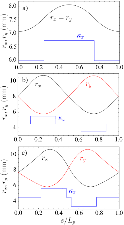
Figure 2: (Color) Example matched envelope solutions for (a) solenoidal, (b) FODO ($\alpha=1/2$) quadrupole, and (c) syncopated ($\alpha=0.1$) quadrupole focusing lattice. Parameters for all cases are: $L_{p}=0.5$ m, $\eta=0.5$, $\sigma_{0}=80^{\circ}$, $Q=4\times 10^{-4}$, and $\varepsilon=50$ mm-mrad. These parameters yield $\sigma/\sigma_{0}=0.3144$, $0.3093$, and $0.3099$ for (a), (b), and (c).

Although the system symmetries assumed simplify interpretation of the matched envelope solutions obtained in the examples, we note that the numerical methods employed in calculation of the particle principal orbits functions and any necessary constraint equations are not structured to take advantage of the symmetries of the matched solutions. Because of this, the examples provide a better guide to the performance of the IM method in situations where there are lesser degrees of system symmetry. MathematicaWolfram (2003) based programs used to in the examples have been archivedLun . These programs can be easily adapted to more complicated lattices.

V.1 Case $1$ and $2$ parameterizations

The IM method described in Sec. IV is applied with $\sigma^{i}=\sigma$ specified and the unknown parameters of the $i$th iteration $\varepsilon^{i}$ (case $1$: $Q$ and $\sigma$ specified) or $Q^{i}$ (case $2$: $\varepsilon$ and $\sigma$ specified) calculated from the constraint equations (34) and (35). The continuous focusing approximation envelope radii $\overline{r_{j}}$ used in the seed ($i=0$) iterations are calculated from Eq. (30) (case 1) and Eq. (28) (case 2). The number of iterations needed to achieve a $10^{-6}$ fractional envelope tolerance [see Eq. (38)] are presented in Fig. 3 as a function of $\sigma_{0}$ and $\sigma/\sigma_{0}$ for solenoidal, FODO quadrupole, and syncopated quadrupole focusing lattices employing both case $1$ and case $2$ parameterization methods. In Fig. 4, iterations corresponding to one data point in Fig. 3 (case $2$ solenoidal focusing) are shown. This example shows a result typical for lower to intermediate values of $\sigma_{0}$, where the seed iteration $r_{j}^{0}$ is fairly close to the matched solution and the first iteration correction $r_{j}^{1}$ closely tracks the matched solution to within a percent local fractional error. Higher values of $\sigma_{0}$ and more complicated lattices result in both seed iterations farther from the matched solution and less rapid convergence with iteration number.

Figure 3: Number of IM iterations needed to achieve a $\mbox{tol}=10^{-6}$ fractional error tolerance matched envelope solution for (a) solenoidal, (b) FODO ($\alpha=1/2$) quadrupole, and (c) syncopated ($\alpha=0.1$) quadrupole focusing lattices as a function of $\sigma_{0}$ (for $\sigma_{0}=40^{\circ}$, $60^{\circ}$, $80^{\circ}$, $\cdots$, $160^{\circ}$) and $\sigma/\sigma_{0}$ (for $\sigma/\sigma_{0}=0.1$, $0.2$, $0.3$, $\cdots$, $1.0$). The left column corresponds to the parametrization case $1$ method with $Q=10^{-4}$ (Unachievable limit points marked x) and the right column corresponds to the parameterization case $2$ method with $\varepsilon=50$ mm-mrad. Other lattice parameters are $L_{p}=0.5$ m and $\eta=0.5$ for (a), (b), and (c).

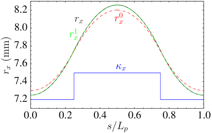
Figure 4: (Color) For solenoidal focusing: converged matched envelope solution (black) with $r_{x}=r_{y}$, the first seed iteration $r_{x}^{0}$ (red), and the second iteration $r_{x}^{1}$ (green). System parameters are $L_{p}=0.5$ m, $\eta=0.5$, $\sigma_{0}=80^{\circ}$, $\varepsilon=50$ mm-mrad, and $\sigma/\sigma_{0}=0.3$.

The data in Fig. 3 shows that the IM method converges rapidly to small tolerances over a broad range of applied focusing ($\sigma_{0}$) and space-charge ($\sigma/\sigma_{0}$) strength. Not surprisingly, stronger focusing strength (i.e., increasing $\sigma_{0}$) requires more iterations for both solenoidal and quadrupole focusing at the fixed value of lattice occupancy $\eta$ employed. Also, lesser degrees of lattice symmetry result in more iterations being necessary for convergence (e.g., lattice convergence rate order: solenoidal, FODO quadrupole, syncopated quadrupole). Iterations required appear to depend only weakly on space-charge strength ($\sigma/\sigma_{0}$) – except for solenoidal focusing lattices with very high $\sigma_{0}$ where required iterations become abruptly larger for weak space-charge with $\sigma/\sigma_{0}$ close to unity. Even parameters deep within the regime of strong envelope instabilityLund and Bukh (2004) converge rapidly. Points for $\sigma/\sigma_{0}=1$ are eliminated in the case $1$ examples because the perveance $Q$ is held to a fixed, finite value and this limit would correspond to a matched beam envelope with infinite cross-sectional area. Conversely, for the limit $\sigma/\sigma_{0}=1$ in the case $2$ examples, only one iteration is required for convergence to a finite solution because for zero space-charge strength the trial seed iteration generated by Eq. (32) for $i=0$ corresponds to the exact matched envelope to numerical error (i.e., when $Q^{0}=0$ the $C_{j}^{0}$ and $S_{j}^{0}$ are the principal undepressed particle orbits which generate the matched envelope of the undepressed beam). The IM method applies for extremely strong space charge with $\sigma/\sigma_{0}\ll 0.1$, but probing the limit $\sigma\rightarrow 0$ requires careful analysis of various terms in the formulation presented in Sec. IV.

Complementary to Fig. 3, the decrease in the log of the fractional tolerance [see Eq. (38)] achieved with iteration number is plotted in Fig. 5 for solenoidal and FODO quadrupole focusing lattices for one set of system parameters. The matched envelopes are calculated using the case $2$ methods. Case $1$ methods and other system parameters yield similar results to those presented. We find that the IM method converges rapidly, with the fractional tolerance achieved increasing by one to two orders of magnitude per iteration till saturating at a value reflecting the precision of numerical calculations employed ($\sim 10^{-15}$ fractional accuracy for the examples in Fig. 5).

Figure 5: Log of fractional error tolerance (tol) achieved for matched envelope solutions versus number of IM iterations for (a) solenoidal and (b) FODO ($\alpha=1/2$) quadrupole focusing lattices. Solutions are generated using case $2$ methods for system parameters: $L_{p}=0.5$ m, $\eta=0.5$, $\sigma_{0}=80^{\circ}$, $\varepsilon=50$ mm-mrad, and $\sigma/\sigma_{0}=0.2$ [corresponding to $Q\simeq 6.700\times 10^{-4}$ and $Q\simeq 6.561\times 10^{-4}$ for (a) and (b)].

V.2 Case $0$ parameterization

In parameterization case $0$, the matched envelope functions $r_{j}$ are specified by $\kappa_{j}$, $Q$, and $\varepsilon_{j}$. For the $i$th iteration, the depressed phase advances $\sigma_{j}^{i}$ needed to calculate the iteration envelope functions $r_{j}^{i}$ are most simply calculated using Eq. (33). Unfortunately, this simple method can fail if space-charge is strong and iterations result in envelope corrections where the radial cross-section of the beam is compressed sufficiently relative to the actual matched envelope solution over the lattice period. Compressive over-corrections can produce iteration principal orbits that are depressed below zero phase advance (i.e., $\sigma_{j}^{i}=0$). In this situation, $\sigma_{j}^{i}$ becomes complex and we find that Eq. (32) can fail to generate an iteration closer to the desired matched envelope solution.

To better understand where the problem described above can occur, a simple continuous focusing estimate (see Sec. III.2) is applied. Taking $\kappa_{j}=(\sigma_{0}/L_{p})^{2}$ and $\varepsilon_{j}=\varepsilon$, we estimate the envelope compression factor $f$ needed to fully depress particle orbits within the matched envelope. A particle moving within the continuous matched envelope $r_{j}=\overline{r_{b}}$ has depressed phase advance $(\sigma/L_{p})^{2}=(\sigma_{0}/L_{p})^{2}-Q/\overline{r_{b}}^{2}$. Replacing $\overline{r_{b}}\rightarrow f\overline{r_{b}}$ and $\sigma\rightarrow 0$ in this phase advance formula gives

$$f=\frac{\sqrt{2}}{\sqrt{1+\sqrt{1+4[\sigma_{0}\varepsilon/(QL_{p})]^{2}}}}.$$ (41)

But for continuous focusing, we haveLund and Bukh (2004)

$$\frac{\sigma_{0}\varepsilon}{QL_{p}}=\frac{(\sigma/\sigma_{0})}{1-(\sigma/\sigma_{0})^{2}}.$$ (42)

Together, Eqs. (41) and (42) show that $f=0.99$, $0.95$, and $0.90$ (corresponding to $\sim 1\%$, $5\%$ and $10\%$ compressive over-corrections) will produce fully depressed particle orbits for $\sigma/\sigma_{0}<0.14$, $0.31$, and $0.44$. Numerically analyzed examples below indicate that this problem can occur in periodic focusing lattices for more moderate space-charge and compression factors than the continuous focusing estimates suggest.

The parameter region where the IM method can be applied using the “conventional” case $0$ procedure for example periodic solenoid and FODO quadrupole lattices is illustrated in Fig. 6. The region of applicability corresponds to parameters where Eq. (33) can be employed to calculate the iteration depressed phases advances $\sigma_{j}^{i}$ without obtaining complex values. Iterations necessary to achieve tolerance are plotted as a function of $\sigma_{0}$ and $\sigma/\sigma_{0}$. Rather than plotting results in terms of the perveance $Q$, Eq. (14) was used to calculate $\sigma/\sigma_{0}$ from the matched envelope functions and system parameters to better quantify the relative space-charge strength where the method fails. Values of $Q$ were chosen to uniformly distribute points in $\sigma/\sigma_{0}$. Note that the IM method works with the simple initial seed iteration when space-charge is moderate to weak ($0.6<\sigma/\sigma_{0}\leq 1$) but abruptly fails with increasing space charge ($\sigma/\sigma_{0}<0.6$). Near the point of failure, convergence becomes slow (iteration counts for the example in Fig. 6 can become thousands if points are chosen sufficiently close to the start of the failure region).

Figure 6: Number of “conventional” IM iterations needed in case $0$ to achieve a $\mbox{tol}=10^{-6}$ fractional error tolerance matched envelope solution for (a) solenoidal and (b) FODO ($\alpha=1/2$) quadrupole lattices as a function of $\sigma_{0}$ (for $\sigma_{0}=40^{\circ}$, $60^{\circ}$, $80^{\circ}$, $\cdots$, $160^{\circ}$) and $\sigma/\sigma_{0}$ (for $\sigma/\sigma_{0}=0.1$, $0.2$, $0.3$, $\cdots$, $1.0$). System parameters are: $L_{p}=0.5$ m, $\eta=0.5$, and $\varepsilon=50$ mm-mrad. Parameters where the method fails are marked x.

Several alternative methods were attempted to render the IM method applicable to all case $0$ parameters with arbitrary space-charge strength. We describe these methods without assuming $\sigma_{0x}=\sigma_{0y}$ and $\varepsilon_{x}=\varepsilon_{y}$ to better reflect general case $0$ applications. First, rather than employing Eq. (33) to calculate the depressed phase advance $\sigma_{j}^{i}$ of the iteration, the integral formula (14) is applied with the envelope functions of the previous $i-1$ iteration with

$$\sigma_{j}^{i}=\varepsilon_{j}\int_{s_{i}}^{s_{i}+L_{p}}\!\frac{ds}{[r_{j}^{i-1}(s)]^{2}}.$$ (43)

The anticipation is that $\sigma_{j}^{i}$ calculated from Eq. (43) should be sufficiently close to the actual depressed phase advance $\sigma_{j}$ of the converged solution to correct the problem. Unfortunately, this method, when applied to example solenoid and quadrupole lattices, results in systematic convergence to unphysical solutions. Replacing Eq. (43) with an “under-relaxed” average over previous iterations might address this problem but was not analyzed. In cases where complex phase advances resulted, various other simple replacements of Eq. (33) were attempted without obtaining satisfactory results.

Several alternative procedures extend applicability to general case $0$ parameters. First, slowly increasing the perveance $Q$ from some sufficiently small (or zero) value while implementing the conventional case $0$ iteration method using Eq. (33) proves workable in our tests. In this scheme, if Eq. (33) fails (i.e., produces unphysical complex values for $\sigma_{j}^{i}$) then $Q$ is adaptively decreased while iterating until the formula becomes valid before increasing $Q$ again toward the target value. For strong space-charge this procedure can result in many iterations being necessary for convergence because small increases in $Q$ were required in various test cases examined. It is also difficult to determine optimal increments to increase the perveance – which complicates practical code development and can limit the range of method applicability.

Another, simpler to implement, alternative procedure is formulated by combining the Sec. V.1 method for solving case $1$ parameterizations with numerical root finding. In this “hybrid” procedure, the emittances $\varepsilon_{j}$ calculated from the $x$- and $y$-plane constraint equations (23) are regarded as an undetermined function of the $\sigma_{j}$ [i.e., $\varepsilon_{j}|_{\text{specified}}=\varepsilon_{j}(\sigma_{x},\sigma_{y})$] and trial matched envelope solutions $r_{j}$ are rapidly calculated to tolerance using matched envelopes obtained with case $1$ methods for specified (guessed) values of the $\sigma_{j}$. Numerical root finding can be employed to refine the guessed values for the $\sigma_{j}$ to obtain the values of $\sigma_{j}$ consistent with the target values of $\varepsilon_{j}$. Because the $\varepsilon_{j}(\sigma_{x},\sigma_{y})$ are smooth, monotonic functions of the $\sigma_{j}$ for $0<\sigma_{j}<\sigma_{0j}$, the consistent values of the $\sigma_{j}$ can be found with relatively small numbers of root finding iterations. This is particularly true for plane-symmetric systems ($\sigma_{0j}=\sigma_{0}$ and $\varepsilon_{j}=\varepsilon$) because one-dimensional root finding can be employed.

The total number of two-dimensional (i.e, the calculations do not assume plane symmetry) iterations needed to implement this hybrid method for case $0$ is shown in Fig. 7 for example periodic solenoid and FODO quadrupole lattices. Here, the total iteration number represents the sum of all iterations needed to calculate the emittances to a specified fractional tolerance while calculating all trial matched envelope solutions to a separate specified tolerance over all two-dimensional root finding steps. The same lattices and presentation methods used in Fig. 6 are employed to aid comparisons. Note that the full case $0$ parameter space is accessible in this procedure with only relatively modest total iteration counts in spite of the additional numerical work resulting from the root finding. A secant-like multi-dimensional root finding method is employedWolfram (2003). Note that only two-dimensional root finding is necessary in contrast to four-dimensional root finding associated with conventional procedures for constructing matched envelope solutions by finding appropriate initial envelope coordinates and angles. Initial root finding iterations are seeded using continuous focusing model estimates for $\sigma_{j}$ calculated from Eq. (28) using the seed values of $\overline{r_{j}}$. Subsequent root finding steps in $\sigma_{j}$ employ the previous step matched envelopes as a seed envelope in the case $1$ iterations. For small root finding steps in $\sigma_{j}$ this previous step seeding saves considerable numerical work. Only one iteration is necessary for the limit points with $\sigma/\sigma_{0}=1$ because for zero space-charge strength the trial seed iteration is exact to numerical error. Iteration counts at fixed $\sigma_{0}$ likely increase and decrease in $\sigma/\sigma_{0}$ due to approximate iteration seed guesses being (accidentally) farther and closer to the actual root than in other cases. If the plane symmetries are employed (i.e., using $\varepsilon_{x}=\varepsilon_{y}$ and $\sigma_{x}=\sigma_{y}$), then total iterations required can be further reduced. Matched envelopes for general case 0 parameters can also be calculated in similar number of total iterations by analogously combining case $2$ methods with numerical root finding. In this case values of $\sigma_{j}$ consistent with specified values of $Q$ are calculated using the two components of Eq. (23) [i.e., set $Q\rightarrow Q_{j}$ in the $j=x$ and $y$ components of Eq. (23) and then root solve for $\sigma_{j}$ consistent with $Q=Q_{j}(\sigma_{x},\sigma_{y})$].

Figure 7: Number of total “hybrid” IM iterations needed for case $0$ using $\mbox{tol}=10^{-6}$ fractional error tolerance case $1$ matched envelope solutions and root found $\varepsilon_{j}$ with $10^{-4}$ fractional accuracy from specified values for (a) solenoidal and (b) FODO ($\alpha=1/2$) quadrupole lattices. The same system parameters and presentation format is employed as is used in Fig. 6.

VI CONCLUSIONS

An iterative matching (IM) method for numerical calculation of the matched beam envelope solutions to the KV equations has been developed. The method is based on orbit consistency conditions between depressed particle orbits within a KV beam distribution and the envelope of orbits making up the distribution. Application of the IM method in simplest form requires numerical solution of linear ordinary differential equations describing principal particle orbits over one lattice period and the calculation of a few axillary integrals over the lattice period. A large basin of convergence enables seeding of the iterations with a simple trial solution that takes into account both the envelope flutter driven by the applied focusing lattice and leading-order space-charge defocusing forces. All cases of envelope parameterizations can be employed, but the method is most naturally expressed, and highly convergent, when employing the depressed particle phase advances $\sigma_{j}$ as parameters — which also corresponds to a natural choice of parameters to employ for enhanced physics understanding. Virtues of the IM method are: it is straightforward to code and applicable to periodic focusing lattices of arbitrary complexity; it is efficient for arbitrary space-charge intensity; and it works for all physically achievable system parameters – even in bands of parametric envelope instability where conventional matching procedures can fail.

Appendix A MATCHED ENVELOPE SYMMETRIES FOR QUADRUPOLE DOUBLET AND SOLENOIDAL FOCUSING

Consider a periodic quadrupole doublet latticeLund and Bukh (2004) focusing a beam with symmetric emittances (i.e., $\varepsilon_{x}=\varepsilon_{y}$). To concretely define doublet focusing, we assume that the lattice focusing functions $\kappa_{j}(s)$ satisfy

$$\kappa_{j}(s)=-\kappa_{j}(-s),$$ (44)

in addition to the general quadrupole lattice symmetry $\kappa_{x}=-\kappa_{y}$. This doublet focusing symmetry is consistent with focusing/defocusing elements with axial structure (i.e., including fringe fields) if both the focusing and defocusing elements are realized by identical hardware assemblies with equal field excitations appropriately arranged in a regular lattice via symmetry operations (i.e., translations and rotations). Without loss of generality, let $s=0$ correspond to the axial location of the drift between two successive quadrupoles in the periodic lattice (for cases where a finite fringe field extends into the drifts, this location will be where $\kappa_{j}=0$). Assume that the matched envelope functions satisfying the KV equations (1) are symmetric about the mid-drift with

$$r_{j}(s)=r_{\tilde{j}}(-s).$$ (45)

Here, if $j=x,y$, then $\tilde{j}=y,x$. Take the $j=x$ KV equation [see Eq. (1)], substitute $s\rightarrow-s$. Then employing the focusing and envelope symmetries in Eqs. (44) and (45) together with $\kappa_{y}=-\kappa_{x}$ obtains the complementary $j=y$ KV equation, thereby showing that the assumed symmetry in Eq. (45) is consistent. An immediate corollary of Eq. (45) is that at any mid-drift between quadrupoles, the envelope is round (i.e., $r_{x}=r_{y}$) with opposite convergence angles (i.e., $r_{x}^{\prime}=-r_{y}^{\prime}$).

Restrict the situation described above to a symmetric FODO system where the two focusing and defocusing quadrupoles are separated by equal length axial driftsLund and Bukh (2004) and the focusing and defocusing elements are each reflection symmetric about their axial midplane [i.e., within one element, $\kappa_{x}(s-\tilde{s})=\kappa_{x}(-s+\tilde{s})$ where $s=\tilde{s}$ is the geometric field center of the element]. These further assumptions lead to the additional FODO focusing symmetry

$$\kappa_{j}(s)=\kappa_{\tilde{j}}(L_{p}/2+s).$$ (46)

With the choice of $s=0$ made as above, the focusing and defocusing optical elements are centered at $s=L_{p}/4$ and $s=3L_{p}/4$ within the period $s\in[0,L_{p}]$. Using steps analogous to those outlined above, it can be shown that the matched envelope functions also have the FODO symmetry:

$$r_{j}(s)=r_{\tilde{j}}(L_{p}/2+s).$$ (47)

Another FODO symmetry can be obtained by replacing $s\rightarrow-s$ in Eq. (47), applying Eq. (45), and differentiating to yield

$$r_{j}^{\prime}(s)=-r_{j}^{\prime}(L_{p}/2-s).$$ (48)

Evaluating this expression at the focusing element centers at $s=L_{p}/4$ and $s=3L_{p}/4$ and invoking periodicity of the $r_{j}$ with $r_{j}^{\prime}(s+L_{p})=r_{j}^{\prime}(s)$ shows that the matched envelope functions are extremized (i.e., $r_{j}^{\prime}=0$) at the focusing element centers in a symmetric FODO lattice. The envelope equations (1) then shows that the $j$-plane extrema of $r_{j}$ with $\kappa_{j}<0$ (defocusing plane) satisfies $r_{j}^{\prime\prime}>0$ and therefore must be a minimum value. Period symmetries then require that the other focusing plane extrema ($\tilde{j}$-plane with $\kappa_{\tilde{j}}>0$) corresponds to a maximum value.

Analogous steps to those employed in the analysis of quadrupole doublet focusing can be applied to solenoidal focusing ($\kappa_{x}=\kappa_{y}$) systems with $\varepsilon_{x}=\varepsilon_{y}$ to show that $r_{x}=r_{y}$. Consider a periodic solenoidal focusing function with only a single element in the period that is also reflection symmetric about the axial midplane (with reflection symmetry defined as for the FODO quadrupole case above). Then procedures used above are readily employed to show that the matched envelope function $r_{j}$ is maximum at the axial center of the focusing element and is minimum at the axial center of the drift.

References

- Kapchinskij and Vladimirskij (1959) I. Kapchinskij and V. Vladimirskij, in Proceedings of the International Conference on High Energy Accelerators and Instrumentation (CERN Scientific Information Service, Geneva, 1959), p. 274.
- Reiser (1994) M. Reiser, Theory and Design of Charged Particle Beams (John Wiley & Sons, Inc., New York, 1994).
- Lund and Bukh (2004) S. M. Lund and B. Bukh, Phys. Rev. Special Topics - Accelerators and Beams 7, 024801 (2004).
- Ryne (1995) R. Ryne, Tech. Rep. acc-phys/9502001, http://arxiv.org, Accelerator Physics (1995).
- Wiedemann (1993) H. Wiedemann, Particle Accelerator Physics: Basic Principles and Linear Beam Dynamics (Springer-Verlag, New York, 1993).
- Lee (1996) E. P. Lee, Particle Accelerators 52, 115 (1996).
- Lee (2002) E. P. Lee, Physics of Plasmas 9, 4301 (2002).
- Anderson (2005a) O. Anderson, in Proceedings of the 2005 Particle Accelerator Conference, Knoxville, TN (IEEE #01CH37268C, Piscataway, NJ 08855, 2005a), p. TPAT061.
- Anderson (2005b) O. A. Anderson (2005b), submitted for publication.
- Davidson (1990) R. C. Davidson, Physics of Nonneutral Plasmas (Addison-Wesley, Reading, MA, 1990), re-released, World Scientific, 2001.
- Hofmann et al. (1983) I. Hofmann, L. J. Laslett, L. Smith, and I. Haber, Particle Accelerators 13, 145 (1983).
- Courant and Snyder (1958) E. D. Courant and H. S. Snyder, Annals of Physics 3, 1 (1958).
- Lee and Briggs (1997) E. Lee and R. J. Briggs, Tech. Rep. LBNL-40774, UC-419, Lawrence Berkeley National Laboratory (1997).
- Davidson and Qian (1994) R. C. Davidson and Q. Qian, Phys. Plasmas 1, 3104 (1994).
- Davidson and Qin (2001) R. C. Davidson and H. Qin, Physics of Intense Charged Particle Beams in High Energy Accelerators (World Scientific, New York, 2001).
- Wolfram (2003) S. Wolfram, The Mathematica Book, 5th ed. (Wolfram Media, 2003).
- (17) Mathematica programs employed can be obtained on the arXiv.org e-Print archive (http://arxiv.org).