Stochasticity of Road Traffic Dynamics:
Comprehensive Linear and Nonlinear Time Series Analysis on High Resolution Freeway Traffic Records

Abstract

The dynamical properties of road traffic time series from North-Rhine Westphalian motorways are investigated. The article shows that road traffic dynamics is well described as a persistent stochastic process with two fixed points representing the freeflow (non-congested) and the congested state regime. These traffic states have different statistical properties, with respect to waiting time distribution, velocity distribution and autocorrelation. Logdifferences of velocity records reveal non-normal, obviously leptocurtic distribution. Further, linear and nonlinear phase-plane based analysis methods yield no evidence for any determinism or deterministic chaos to be involved in traffic dynamics on shorter than diurnal time scales. Several Hurst-exponent estimators indicate long-range dependence for the free flow state.
Finally, our results are not in accordance to the typical heuristic fingerprints of self-organized criticality. We suggest the more simplistic assumption of a non-critical phase transition between freeflow and congested traffic.

I Introduction

Traffic flow prediction, particularly in close connection with the avoidance of jams, is a challenging, yet hitherto unreached target.
Until now, due to restricted access to records, simulation models provided the predominant approach to understand traffic dynamics. Several approaches have been developed which are based on partial differential equations (Helbing (2001a),Kerner and S.Klenov (2002)), or cellular automata models as the widespread Nagel-Schreckenberg model (Schadschneider (1999)). A comprehensive overview of results from time series analysis from real traffic records was published by Helbing (2001b). In earlier research on the database that our study relies on, diurnal, weekly and annual cycles in traffic density as well as velocity was reported in details by Chrobok (2000). Autocorrelation and time-headways of traffic records are demonstrated to vary state-dependently (Knospe et al. (2002),Neubert et al. (1999)), congested traffic revealing a more persistant autocorrelation.
Intuitively, traffic dynamics conforms rather to a stochastic than deterministic(-chaotic) process. A rigorous statistical inference however, to the best of our knowledge has not yet been achieved.

This paper is organized as follows: We first introduce the dynamical phase-plane reconstruction from traffic records by fundamental diagram and delay-plot, to point up that traffic dynamics consist of two heterogeneous states. The further analysis focuses on separated sections of either free flow or congested traffic regimes.
We then turn to phase-plane based methods such as correlation integrals, and surrogate based local linear predictions to demonstrate that traffic dynamics on below diurnal time scales has a predominantly stochastic nature.
Long-range dependence is tested from several measures. To exclude possible effects of nonstationarity, the latter measure is compared with appropriate phase randomized surrogates. Nonlinearity will be discussed by application of the surrogate based time-reversibility test.

II Data Analysis

II.1 Methods

II.1.1 Phase-randomized surrogates

In time series analysis, phase-randomized surrogate (PRS) time series (Theiler et al. (1992)) can be applied as a version of bootstrapping to clarify and quantify statements about the presence of nonlinear effects. PRS series reveal the same linear statistical properties as their original and can be produced at will. Possible nonlinearities, as nonlinear determinism beyond the autocorrelation of the original time series will not be reproduced by their surrogatization, or changed by interpretation as a spectral property.
In summary, PRS time series are produced by multiplying the Fourier-spectrum of the original records with random phases and hereafter performing a backtransformation (for details see Timmer et al. (2000) or Kantz and Schreiber (1997)).

II.1.2 Nonlinear methods

In this paper we will make use of linear and nonlinear phase-plane based measures such as correlation dimension and local linear prediction. Such methods are usually applied to time series with the intention of identifying the presence of nonlinear, possibly chaotic dynamics. Since it is hardly possible to formally prove the absence of any deterministic property, we intend to point out this absence by comparing (nonlinear) statistics for original data vs. their appropriate surrogate substitutes.

II.2 Records

Freeway traffic in North-Rhine Westphalia (Germany) is continuously monitored at approximately 1400 road locations by means of built-in loop detectors. For every appearance of a vehicle these detectors record:

1. time,

2. velocity,

3. type of vehicle,

4. length of the vehicle.

This study is based on two different types of static loop-detector recordings:

1. Single car records:
   Only a few exceptional time series have been recorded with a notebook PC attached to the loop detectors,

2. minute-aggregated data:
   These data are obtained from the same loop detectors as single- car data. However, instead of immediate recording, the samplings are exponentially smoothed and aggregated in 1-minute intervals.

Both single-car and minute aggregated records are coarse-grained, since all records are denoted in $[$ ”0” $\ldots$ ”254” $]$, while ”255” denotes faulty results. Due to their higher resolution, single-car data provide rare, but the most detailled (and unspoilt) information, particularly for short time scales.
For more details of sampling and processing read Knospe et al. (2002) and Neubert et al. (1999). Both articles provide a detailled introduction into practial aspects of road traffic data.

III Results

III.1 Time course of traffic dynamics

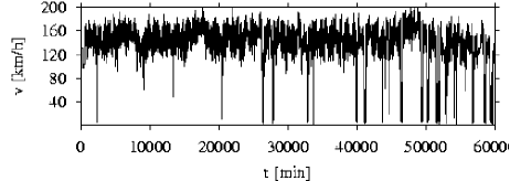
(a)

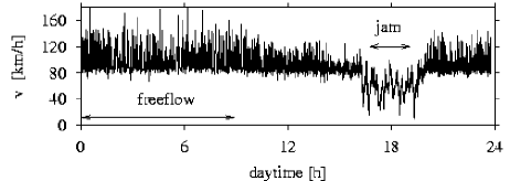
(b)

Figure 1: velocities,
a) minute aggregated records, covering 60.000 min $\approx$ 1000 h $\approx$ 40 d.
(b) 1 day of single car data comprising a jam event, arrows indicate sections of jam and freeflow traffic state that will be analyzed in the following.

Fig. 1 presents a section of typical single car freeway traffic records. In a), the velocity time series appears more or less regularly fluctuating, except for occasional abrupt drops in velocity, (b) is a one-day sequence of single-car records comprising a jam episode.

III.1.1 Fundamental diagram

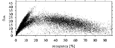
Figure 2: Fundamental diagram: plot of occupancy $[$sum of vehicle lengthes per road kilometer$]$ vs. flux $[$vehicles per minute$]$ for minute aggregated traffic records.

In the context of traffic analysis, the fundamental diagram, well known to applied scientists, denotes the plot of flux vs. occupancy, in most cases graphed from smoothed model output data (e.g. Wagner (1995)) .
Fig. 2 was graphed from minute aggregated records. Due to the discreteness of the latter, in a plot like Fig. 2, some hundreds of thousands of data would fall into a few bins. To improve the visualization, we added uniformly distributed independent random noise $[-0.5<\xi<0.5]$ (the noise level scales below the resolution of the signal) to the data. Fig. 2 gives an impression of traffic dynamics, that undergoes transitions between two attractive regions representing freeflow and jammed state. Whereas the freeflow regime (high velocity, low occupancy) is situated transversally on the left hand side, the congested state associates with a larger realm of points in the center and on the right hand side.

III.2 Delay plot

Fig. 2 can be interpreted as ”phase plane” formed from records. An alternative, more practicable method to obtain a comparable clue on phase plane is delay coordinate embedding, which denotes a $n$-dimensional plot $x_{t}$ vs. $x_{t+\tau}$ vs. $\ldots$ vs. $x_{t+n\tau},n\ll N$ of a time series $x_{t},t=1,2,\ldots N$.
The well-known general results by Takens Takens (1980) state that the dynamics of a system recovered by delay coordinate embedding are comparable to the dynamics of the original system. A low dimensional deterministic-chaotic attractor thus can be graphed from each of its observed variables as a topologically equivalent structure to what one would obtain from the graph of its variables in a sufficiently dimensioned delay plot. Since there is no straightforward way to determine which dimension is sufficiently large, several dimensions need to be examined. According to Kantz and Schreiber (1997) an optimal delay $\tau$ approximately corresponds to the empirical autocorrelation function (ACF) at $r(\tau)=1/e$. Fig. 3a) shows a delay plot of the velocity series $x_{t}$ used in Fig. 2, here plotted in time-delayed coordinates $x(t-\tau)$, $x(t)$ and $x(t+\tau)$, $\tau>0$ denoting the delay-time. In Fig. 3 (a) and (b) the data scatter around two condensed regions, which can be identified as congested and freeflow traffic.
We present Fig. 3 to visualize a clearer two fixed-point structure than in the ”traditional” plot Fig. 2. Moreover, though the single car data base is not sufficient to obtain a fundamental diagram, Fig. 3 (b) gives an indication of comparable dynamics in single car data.

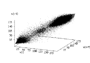
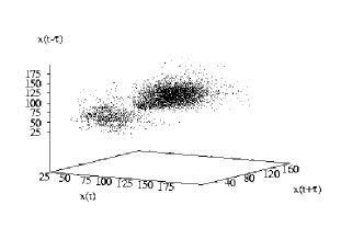
(a) (b)

Figure 3:
(a) Delay-plot minute aggregated velocity data covering one month, $\tau=1$ minute.
(b) Delay plot of single-car data - (1 day), $\tau=25$ sec.

III.2.1 Local stationarity assumption

Naturally, the double fixed point structure, visualized in figures 2 and 3, gives a strong indication against stationarity for the overall process of traffic dynamics that comprises two traffic states. In the following we will therefore constrain the analysis to selected sections of either freeflow or jammed traffic that are indicated by arrows in Fig. 1. To apply methods that require regularly sampled data we transform these sections of single-car data equidistant by aggregation and linear interpolation, expecting that this procedure does not have substantial influence on the results.

III.3 Distribution of intervals between consecutive events (time-headways)

Time-headway distributions from single car data have already been reported in Neubert et al. (1999) for different traffic states. According to our results they reveal an approximately lognormal distribution with different parameters in dependence of the traffic state (Fig.4 (a) and (b)). For freeflow traffic the Kolmogorov-Smirnov test statistics

$$\hat{D}=\frac{|x_{min}-x_{max}|}{n=500}=0.0000804$$ (1)

performs below the tabelled value

$$D_{\alpha=0.001}=\frac{1.949}{\sqrt{n=500}}=0.087.$$ (2)

Thus, this test on distributional adaptation does not state the rejection of the null-hypothesis of lognormal distribution. In Fig. 4(a) however, a deviation in the right wing (reminding to a fat tail) is observed. The finite left tail of the distributions probably reflects the necessity to keep a security distance between vehicles. Data of jammed traffic (Figure 4(b)) are comparably scarce. Little, if anything, can be inferred from them.

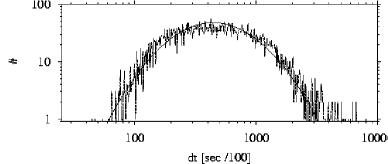
(a) (b)

Figure 4: (a) Time interval histogram of entire single car data series (dashed line), fitted lognormal distribution (solid line)). (b) Time interval histogram during jammed state, fitted lognormal distribution (dashed line).

III.4 Self Organized Criticality

Previous authors (Paczuski and Nagel (1995)) already suspected that road traffic has a selfsimilar nature in the context of the Self- Organized Criticality (SOC) models. According to such models, increasing traffic load would produce a ”critical” situation, that, at its critical point, occasionally relaxes catastrophically (e.g. as sandslides in the sandpile model Bak et al. (1988)). Close to the critical point, such a system generates power law behaviour, observable in leptocurtic distributions, slowly converging variance, lack of characteristical scales and 1/f noise.

III.4.1 Distribution of velocities and velocity differences

Figure 5: Histogram of single car velocities of 12 different single-car highway traffic data sources (solid line),
interpretation as addition of 2 Gaussian distribution curves (dashed line).

(a) (b)

Figure 6: (a) Histogram of differenced single car velocities selected for jam and freeflow epsidodes,
(b) cumulated distribution of logdifferenced single car velocities selected for left(l) and right (r) wings.

Fig. 5 shows the histogram of traffic velocities of all single-car data (12 different locations). In some locations slow congested traffic and jams appear as a smaller second peak that, e.g. for smaller data quantity, could be misinterpreted as fat tail in the low-speed end of the empirical velocity probability distribution function.
Comparable to the well-known heavy-tailed distributions of logdifferenced financial time series, in fig. 6 (a) we observe a clearly non-normal distribution in differenced velocity records, separated for either jam and free-flow records. This holds for logdifferenced data as well (not shown here). The histogram looks more leptocurtic for free-flow than for jammed traffic records.
The plot of the cumulated distribution function in double-log coordinates provides a clue if the asymptotic behaviour of the functional form of the cumulative distribution is ”visually” consistent with a power law,

$$P(G>x_{*})\approx\frac{1}{x^{\alpha}}$$ (3)

where $\alpha$ is the exponent caracterizing the power law decay,

$$G(t,\Delta t)\equiv\ln(x_{t+\Delta t})-\ln(x_{t})$$ (4)

(Plerou et al. (1999)). Together with other indications, such a power law can be regarded as a feature which is characteristic for SOC processes (Jensen (1998)).
Conversely, the cumulated distribution of differenced velocities, separated for right and left wings of either jam and freeflow records, displays no clear scaling region. Non-normal distribution as well as lack of scaling is also observable for the larger database of minute aggregated records (not shown here).

III.5 Long-range dependence

Scientists in diverse fields observed empirically that positive correlations between observations which are far apart in time decay much slower than would be expected from classical stochastic models. In time series such correlations are characterized by the Hurst exponent $H$. They are often referred to as Hurst effect or long-range dependence (LRD). $0.5<H<1$ reflects long-range positive correlations between sequential data. $H=0.5$ corresponds to sequential uncorrelatedness (known for white noise). Brownian motion, the trail of white noise, is characterized by $H=1$.
Since long-range dependence (LRD) is defined by the autocorrelation function (ACF), theoretically, the shape of the ACF provides an indication for LRD in road traffic. For LRD series, the ACF at large lags should have a hyperbolical shape:

$$r(\tau)\propto\tau^{2H-2},\tau\rightarrow\infty$$ (5)

(Taqqu et al. (1995)).
The practical ability to assure an algebraic decay of the ACF however is low, making such an approach inviable for data analysis. For comparable reasons, from the tail of the distribution, additional information is hardly obtainable; statistics here are generally poor (Carreras et al. (1999)). The discreteness of car traffic data additionally diminishes the quality of such estimations.

III.5.1 Hurst-exponent estimation

The estimation of the Hurst-exponent ($H$) from empirical data is not a simple task. Several studies (e.g. Taqqu et al. (1995),Molnar and Dang (2000),Bates and McLaughlin (1996)) estimate the Hurst exponent $H$ from different measures.
Synthetically generated fractional Brownian motion or fractional ARIMA (autoregressive integrated moving average) series are characterized by a generalized (or global) $H$. Such so called monofractional series are known to reveal fluctuations on all time scales.
They will produce unambiguous evidence for fractionality, whereas a more general class of heterogeneous signals exist that are made up of many interwoven sets with different local Hurst exponents, called multifractional (Latka et al. (2002)). It is a frequent experience, that graphical methods to test for LRD show no clear scaling for such series. Our own experience is, that weighted sums of synthetically generated random walks with different characteristical scales may as well reveal straight fractional scaling in some plots, as crossover behaviour according to other methods. Furthermore, some methods of $H$-estimation sensitively depend on the distribution of the data.
The main criticism against $H$-estimates is based on the experience that instationary data may, at least in some cases, produce estimates that erroneously indicate fractionality. Thus, we are interested in the robustness of $H$-estimators, if possible effects of instationarity are excluded. Phase-randomized surrogates (PRS) based on original traffic records are random sequences with the same first and second order properties (the mean, the variance and the auto-covariance data, but which are otherwise random.
Since fractionality is a spectral property, and PRS fully recover the latter, $H$-estimation of PRS hence provides an approach to exclude possibly misleading effecs of instationarity, albeit not to differentiate between monofractional and heterogeneous signals.

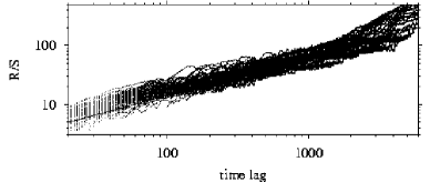
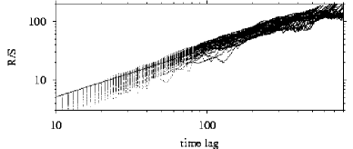
(a) (b)

Figure 7:
R/S pox plot of (a) freeflow and
(b) congested velocity records, approximation of scaling by Hurst exponents (a) $H=0.71$, (b) $H=0.81$ (solid lines).

(a) (b)

Figure 8:
(a) Spectrum from selected freeflow series (dots), exponentially weighted moving average (solid line), scale exponents $\alpha\approx 0.71,$ (dashed line).
(b) Spectrum from selected jam series (dots), exponentially weighted moving average (solid line), scale exponent $\alpha=0.88$ (dashed line)

To obtain reliable H-estimates despite possible effects of nonstationarity, we apply a variety of the most familiar methods to jam- and freeflow traffic records. For a detailled discussion about the application of methods to conclude on LRD, e.g. aggregated variance method, R/S plot, periodogram method and wavelet-based Whittle-estimator on nonstationary data read Molnar and Dang (2000). Detrended fluctuation analysis (DFA) (Peng et al. (1995)) denotes the root mean square fluctuations

$$F(n)=\sqrt{N^{-1}\sum_{k=1}^{N}[y(k)-y_{n}(k)]^{2}}$$ (6)

around least squares line trend fits $y_{n}(k)$ for equal box length $n$ of the integrated series

$$y(k)=\sum_{i=1}^{k}(x_{i}-\bar{x}),\qquad\bar{x}=N^{-1}\sum^{N}_{i=1}.$$ (7)

A straight line in the double logaritmic plot that indicates scaling has the slope $2H$. The method should provide robust estimates even for nonstationary time series. Table 1 displays the results.
We also applied the wavelet-based Whittle estimator (Abry and Veitch (1998)). Despite its postulated robustness against instationarity, and despite $H$-estimates that compare to table 1, we do not show the graphs here, since, particularly for the jam series, the wavelet-spectrum offers to many possibilities of parametrization, as. e.g. the choice of the wavelet function, octaves etc..

est.	freeflow	$\sigma$	jam	$\sigma$
R/S	$0.657$		$0.823$
” for PRS	$0.656$	$0.012$	$0.842$	$0.016$
a.v.	$0.761$		$0.89$
” for PRS	$0.779$	$0.022$	$0.896$	$0.041$
a.a.	$0.522$		$0.669$
” for PRS	$0.511$	$0.002$	$0.586$	$0.035$
spc.	$0.611$		$0.875$
DFA	$0.685$		$1.107$
” for PRS	$0.669$	$0.005$	$1.232$	$0.017$

Table 1: Hurst-exponent estimators from traffic records for different methods: R/S : rescaled range analysis,
a.v.: aggregated variance method,
a.a.: aggregated absolutes,
spc.: graphical estimation from the spectrum,
DFA: detrended fluctuation analysis. PRS denotes the application of the above methode to phase-randomized surrogates,
$\sigma$ denotes the standard deviation.

Fig. 7 presents the R/S pox plots of freeflow and jam records. Particularly for freeflow data exact straight scaling is not observable. The same, even more, holds for Fig. 8 a). In anaogy to the the modified periodogram method outlined in Taqqu et al. (1995), the logaritmically spaced spectrum was divided into 60 boxes of equal length. The least squares ft was performed to averages of the data inside these boxes, to compensate for the fact that most of the frequencies in the spectrum fall on the far right, whereas for LRD-investigation the low frequencies are of interest. Fig. 8(a) gives the strongest indication that traffic dynamics can not be characterized as monofractional as most of the common Hurst-estimators would indicate.

III.6 Time reversibility test

An important property to differentiate between linear and nonlinear stochastic processes is time-reversibility, i.e. the statistical properties are the same forward and backward in time. From this test one can not judge whether the data correspond to any ARMA-model, since theoretically, time asymmetry might be caused by non-Gaussian innovations. Apart from on-ramps, traffic dynamics on short time scales anyway is unlikely to be substantially influenced by external noise.
The following expression is outlined as a measure to conclude on time reversibility of time series (Theiler et al. (1992)):

$$Q(\tau)=\frac{E[(x_{t+\tau}-x_{t})^{3}]}{E[(x_{t+\tau}-x_{t})^{2}]},$$ (8)

wherein $\tau$ denotes the delay time and $E$ represents the time average. The basic idea behind it is to compare the time reversibility test statistics of the original data $Q(\tau)$ with confidence bounds from corresponding test statistics $Q_{sur}(\tau)$, generated from surrogate series:

$$Q_{surr}(c^{\prime}_{\alpha},\tau)<Q(\tau)<Q_{surr}(c_{\alpha},\tau);$$ (9)

for some critical $c^{\prime}_{\alpha};c_{\alpha}$.
The results for a surrogate-based test are usually reported as significances:

$$S(\tau)=\frac{\sqrt{(Q(\tau)-\langle Q(\tau)\rangle_{surr})^{2}}}{\sigma(Q(\tau))_{surr}},$$ (10)

where:
$Q(\tau)$ test statistics, $\langle Q(\tau)\rangle_{surr}$ mean, $\sigma(Q(\tau))_{surr}$ standard deviation.
The test is based on the assumption that the surrogate test statistics for a given lag are approximately Gaussian distributed.
The statistical properties of the examined surrogate time series are the same forward and backward in time. Thus they comply with the null-hypothesis of time-reversibility which will be tried to reject by the test.
The evaluation of significances for more than one lag leads to the statistical problem of multiple testing. This has severe implications on the probability to reject the null-hypothesis. The Bonferroni-correction of the significance level must be taken into account:

$$\hat{\alpha}=1-(1-\alpha)^{n}.$$ (11)

wherein $n$ denotes the number of independent tests. Practically, Bonferroni- corrected confidence bands render little diagnostic power to detect a violation of the null-hypothesis. A corrected significance level, for example, $1-\hat{\alpha}=0.95$ for $100$ independent tests requires $1-\alpha\approx 0.9995$. In most cases, however, $Q(\tau)$ is autocorrelated to an unknown extent, what diminishes the number of independent tests and, for rejection of the null-hypothesis, results in a conservative test design.
In Fig. 9, surrogate-based time-reversibility tests for jam and freeflow traffic states are graphed. Under the assumption of 100 independent tests for $\alpha=0.001$, the corrected significance level is: $\hat{\alpha}=1-(0.9999)^{n=100}\approx 0.905,$ which, though not acceptable as safe statistical inference, gives a vague information that freeflow traffic dynamics is more likely time-irreversible than time-reversible. For the jammed state the observed 20 deviations of the confidence bands gives a comfortably safe rejection of the null-hyothesis, particularly for short time scales, but also for larger $\tau$. Since, even for the naked eye, the test statistics is substantially correlated, the test provides a safe rejection. For the freeflow state, 14 deviations from $H_{0}$ are also statistically indicative, albeit less correlation among the test statistics is observable. Both traffic states thus are likely to reveal time-irreversible statistical properties.

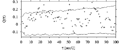
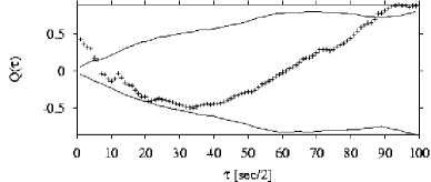
(a) (b)

Figure 9:   (a) $Q(\tau)$ from freeflow series (crosses), lines indicate confidence limits from 500 surrogate realizations. (b) $Q(\tau)$ from jam traffic series (crosses), lines indicate confidence limits from 50 surrogate realizations.

III.7 Recurrence plot

For a time series $x_{t}$ the recurrence plot is a two-dimensional graph that is formed from embedded vectors

$$\vec{y}(t)=(x_{t},x_{t+\tau},\ldots,x_{t+(E-1)\tau})$$ (12)

for embedding dimension $E$ and lag $\tau$. These vectors are compared if they are in $\epsilon$-proximity of another $\vec{y}(t+\Delta t)$.
If

$$||\vec{y}(t)-\vec{y}(t+\Delta t)||<\epsilon,$$ (13)

a black point is drawn at $(t,\Delta t)$. For each $\epsilon,\tau,m$ (with: $m$ the embedding dimension, $\tau$ the time lag, $\epsilon$ the variable error distance) an individual recurrence plot is obtainable.
Since the differences

$$\vec{y}(t_{i})-\vec{y}(t_{j})=c_{i,j}=c_{j,i}=\vec{y}(t_{j})-\vec{y}(t_{i})$$ (14)

are identical, the plot consists of two symmetric triangular graphs along a black (since $i=j$) diagonal line.
Except for horizontal and vertical stripes (that might reflect temporal (auto-) correlations), the recurrence plot of freeflow traffic Fig. 10 is very much in remedy of what one would observe for a recurrence plot of a white noise series.

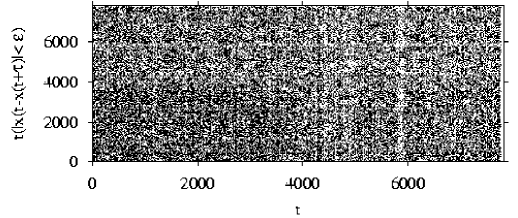
Figure 10: Recurrence plot of freeflow data, $\tau=1.7$ seconds, $\epsilon=0.01$, $m=3.$

III.8 Correlation integral

There exist

$$N_{T}=\frac{1}{2}N(N-1)$$

independent radii $c_{n,m}$ (since $c_{n,m}=c_{m,n}).$ The density of a recurrence plot as functional of $\epsilon$

$$C(\epsilon,D,\tau)=1/N_{T}\sum_{t=1}^{t=N}\sum_{\tau=1}^{n-1}\theta(\epsilon-|x_{t}-x_{t-\tau}|_{E})$$ (15)

($\theta$ denoting the Heavyside step function,
with $\theta(z)=1,$ for $z>0,\,\,\,\,\theta(z)=0$ for $z\leq 0$)
is called the correlation integral. The resulting $C_{r}(\epsilon)$ is sketched in a double logarithmical Grassberger-Procaccia plot (Grassberger and Procaccia (1983)) in dependence of $\epsilon$.
The correlation integral is plotted for varying dimension as well as varying $\epsilon$. If a noise-contaminated deterministic process is regarded, from a sufficient embedding dimension, parallel slopes for varying dimensions indicate power law scaling in a region which is situated above a certain $\epsilon$ that represents the noise range.

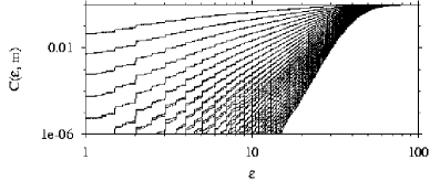
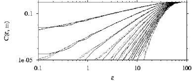
(a) (b)

Figure 11:
a) Grassberger-Procaccia plot for (a) freeflow- and (b) jammed state traffic data for varying dimensions and lag $\tau=7$ seconds (solid lines). Grassberger-Procaccia with identical parameters for appropriate surrogate series realizations are plotted in dashed lines.

Figure 11 shows Grassberger-Procaccia plots for (a) free flow traffic and (b) jammed state records for error distances $\epsilon$ of values $0.1\ldots 100$ and embedding dimension $2\ldots 25$. Both graphs fail to reveal any scaling region, moreover there is obviously no difference to Grassberger-Procaccia plots of appropriate surrogate realizations.
The dimensions of merely stochastic systems appear infinite, therefore for this case it is a typical result, that the correlation integral reveals the embedding dimension (Hegger et al. (1999)).

III.8.1 Casdagli test

The local linear prediction of a time series in delay representation $\underline{x_{t}}$ is achieved by determination of a matrix $A$ that minimizes the prediction error:

$$\sigma^{2}=\sum_{\underline{x}_{t}\in{\cal U}_{t}}(\underline{x}_{t+1}-A\underline{x}_{t}-b_{t})^{2}.$$ (16)

where ${\cal U}_{t}$ denotes the $\epsilon-$ neighbourhood of $\underline{x_{t}}$ excluding $\underline{x_{t}}$ itself. In some analogy to linear regression the prediction is:

$$\underline{x}_{t+1}^{*}=A\underline{x}_{t}+b_{t}.$$ (17)

Local linear models are suggested a test for nonlinearity (Casdagli and S. Eubank (1989)). The average forecast error is computed as function of the neighbourhood size on which the fit is performed. If the optimum occurs at large neighbourhood sizes, the data are (in this embedding) best described by a linear stochastic process, whereas an optimum at rather small neighbourhood sizes supports the idea of existence of a nonlinear, almost deterministic, equation of motion (Hegger et al. (1999)).

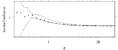
(a) (b)

Figure 12: Casdagli plot of (a) free-flow and (b) jammed state traffic data (crosses), compared to confidence bands, generated from to PRS series (dotted lines).

In Fig. 12 the Casdagli-test was performed for original as well as for surrogate data. In the context of the Casdagli-test it is meaningless some of jam records fall not within the surrogate-based confidence intervals. The qualitative comparability gives an indication for predominant stochasticity particularly in freeflow traffic records.

IV Discussion

According to our analysis of traffic records, traffic dynamics is a two fixed point stochastic process, while the fixed points reflect the jam and freeflow regime.
The abrupt transitions between the traffic states imply nonlinearity in the overall traffic dynamics. A variety of methods, more or less sensitive towards nonstationarity, yields Hurst-exponents that indicate long-range dependent dynamics in particular for freeflow traffic. Differenced as well as logdifferenced velocity records reveal heavy tailed distribution, however for both there is no clear scaling region observabele to estimate scaling exponents.
From our results it must be concluded that below diurnal time scales traffic data in jammed as in freeflow state exhibit neither deterministic nor low dimensional chaotic properties.
The main intention of this article is to outline an overview of the stochastical properties achieved by data analysis of single-car road traffic records.
Attending the problem of criticality in road traffic records, we find that as well the two fixed-point dynamics as the distribution of (differenced) velocities are contrary to the typical features of processes governed by self-organized criticality. This lets us rather suspect the rise of jams in the context of a (eventually, but not necessarily, critical) phenomenon linked to a phase-transition. For such a model hypothesis, known e.g. in equilibrium thermodynamics, the point of transition can be reached by fine tuning of a parameter. This must be distinguished from self-organized criticality, which represents the classification for systems attracted permanently by variable critical states.
Contrary to the well-known conceptual analogy between traffic and granular flow, we rather propose an intuitive analogy of traffic dynamics with the condensation of steam to water. In contrast to the condensation of water driven by withdrawal of heat, free flow traffic condenses to higher particle density by an increase of trafficants in this picture. This increase can be interpreted as rised pressure. In accordance to such considerations and the empirical results of Helbing (2001b) increasing traffic load (or input to the motorway) produces a (in the more popular sense) ”critical” tension that relaxes in an abrupt transition to a jam. In this instructive example, traffic accidents, construction sites or slow vehicles could act comparable to condensation cores by exerting strong nonlinear negative feedback on the upstream traffic. The fine tuning parameter thus is the capacitiy of the motorway, limited by traffic load, accidents or construction sites.

References

- Helbing (2001a) D. Helbing, Mathematical and Computer Modelling 35, 517 (2001a).
- Kerner and S.Klenov (2002) B. Kerner and S.Klenov, J. Phys. A: Math. Gen. (2002).
- Schadschneider (1999) A. Schadschneider, European Physical Journal B 10, 573 (1999).
- Helbing (2001b) D. Helbing, Reviews of Modern Physics 72, 1067 (2001b).
- Chrobok (2000) R. Chrobok, Master’s thesis, University of Duisburg (2000), URL traffic.uni-duisburg.de/chrobok.ps.
- Knospe et al. (2002) W. Knospe, L. Santen, A. Schadschneider, and M. Schreckenberg, Phys. Rev. E 65 (2002).
- Neubert et al. (1999) L. Neubert, L. Santen, A. Schadschneider, and M. Schreckenberg, Phys. Review E 60 (1999).
- Theiler et al. (1992) J. Theiler, S. Eubank, A. Longtin, B. Galdrikian, and J. D. Farmer, Physica D 58, 77 (1992).
- Timmer et al. (2000) J. Timmer, U.Schwarz, H. Vos, I. Wardinski, T. Belloni, G. Hasinger, M. van der Klis, and J. Kurths, Physical Review E 61, 1342 (2000).
- Kantz and Schreiber (1997) H. Kantz and T. Schreiber, Nonlinear Time Series Analysis (Cambridge Univ. Press, Cambridge, England, 1997).
- Wagner (1995) P. Wagner, in Workshop on Traffic and Granular Flow, HLRZ, Jülich, Germany (World Scientific, Singapore / New Jersey / London / HongKong, 1995), iSBN 981-02-2635-7.
- Takens (1980) F. Takens, Lecture Notes in Mathematics 898, pp 366 (1980).
- Paczuski and Nagel (1995) M. Paczuski and K. Nagel, in Workshop on Traffic and Granular Flow, HLRZ, Jülich, Germany (World Scientific, Singapore / New Jersey / London / HongKong, 1995), iSBN 981-02-2635-7.
- Bak et al. (1988) P. Bak, C. Tang, and K. Wiesenfeld, Phys. Rev. A 38, 364 (1988).
- Plerou et al. (1999) V. Plerou, P. Gopikrishnan, L. Amaral, M. Meyer, and H. E. Stanley, Physical Review E 60, 6519 (1999).
- Jensen (1998) H. J. Jensen, Self Organized Criticality, Emergent Complex Behaviour in Physical and Biological Systems (Cambridge Lecture Notes in Physics, Cambrigde, England, 1998).
- Taqqu et al. (1995) M. Taqqu, V. Teverovsky, and W. Willinger, Fractals 3, 785 (1995), http://citeseer.nj.nec.com/34130.html.
- Carreras et al. (1999) B. Carreras, B. P. van Milligen, M. Pedrosa, R. Balbin, C. Hidalgo, D. Newman, E. Sanchez, I. Garc a-Cortes, J. Bleuel, M. Endler, et al., Physics of Plasmas 6 (1999), URL www-fusion.ciemat.es/fusion/personal/boudewijn/PDFs/conferenc%es/EPS98.pdf.
- Molnar and Dang (2000) S. Molnar and T. D. Dang, Pitfalls in long range dependence testing and estimation (2000), URL citeseer.ist.psu.edu/molnar00pitfalls.html.
- Bates and McLaughlin (1996) S. Bates and S. McLaughlin, An investigation of the impulsive nature of ethernet data using stable distributions (1996), URL citeseer.ist.psu.edu/bates96investigation.html.
- Latka et al. (2002) M. Latka, M. Glaubic-Latka, D. Latka, and B. West, arXiv:physics (2002).
- Peng et al. (1995) C.-K. Peng, H. S, H. Stanley, and A. Goldberger, Chaos 5, 82 (1995).
- Abry and Veitch (1998) P. Abry and D. Veitch, IEEE Transactions on Information Theory 44, 2 (1998).
- Grassberger and Procaccia (1983) P. Grassberger and I. Procaccia, Phys. Rev. Lett. 50, 346 (1983).
- Hegger et al. (1999) R. Hegger, H. Kantz, and T. Schreiber, CHAOS 9, 413 (1999).
- Casdagli and S. Eubank (1989) M. Casdagli and e. S. Eubank, Physica D 35, 357 (1989).