Controlling Strong Electromagnetic Fields at a Sub-Wavelength Scale .

Abstract

We investigate the optical response of two sub-wavelength grooves on a metallic screen, separated by a sub-wavelength distance. We show that the Fabry-Perot-like mode, already observed in one-dimensional periodic gratings and known for a single slit, splits into two resonances in our system : a symmetrical mode with a small Q-factor, and an antisymmetric one which leads to a much stronger light enhancement. This behavior results from the near-field coupling of the grooves. Moreover, the use of a second incident wave allows to control the localization of the photons in the groove of our choice, depending on the phase difference between the two incident waves. The system exactly acts as a sub-wavelength optical switch operated from far-field.

Surface Enhancement Raman Scattering (SERS) still remains a mystery in a large part, even though it is now accepted that the excitation of localized electromagnetic modes of irregular metallic surfaces is involved in its basic mechanismotto; moskovits . Optical excitation of such modes can indeed lead to important concentration of electromagnetic energy in volumes (cavities) much smaller than $\lambda^{3}$ where $\lambda$ is the excitation wavelength, as it is the case for SERS active surfaces. These specific places of very strong electromagnetic fields localization are called ”active sites” or ”hot spots”. However, the debate on the origin of these hot spots remains open, as well as the hope to control one day this phenomenon. The large interest raised by this fundamental physics is also increased by its wide potential applications in biochips, sensors, nano-antennae, optoelectronics or energy transport on nanostructured surfaces.

In this letter, we consider a simple system which allows to produce and control the localization in space of such hot spot phenomenon. It only consists of two deep grooves on a plane metallic gold surface (fig.1). The excited modes appear, for the chosen geometry, in the infrared region where we can consider the metal as being a good reflector. Under this condition, a reliable theoretical method, i.e the modal method using surface impedance boundary conditions, can be used wirgin . This method has already demonstrated its ability to give a good qualitative and quantitative agreement with the measured reflectivity of metallic gratings barbara1 ; barbara2 ; barbara3 . The case of one groove only was considered a long time ago deleuil , while the transmission for one takakura and two slits schouten were only recently considered. In contrast with schouten , the distance between our two grooves is small with respect to the incident wavelength. Very recently it also was shown skigin that sharp and deep resonances appear in the transmission response of gratings with more than one slit per period or in gold dipole antennasmartin . We here analyze the physical origin of this new kind of resonances for a two slit system. As we will see, this allows us to point out some very fundamental aspects of electromagnetic resonances on metallic surfaces, and to control the light localization by using a simple device.

We consider a p-polarized incident plane wave (electric field in the plane of incidence) with a wavevector $k=2\pi/\lambda$ impinging on the surface at an angle $\theta$ (fig.1). The knowledge of the magnetic field in the $z$-direction completely solves the problem as $H_{x}=H_{y}=E_{z}=0$, $E_{x}=(i/ck\varepsilon_{0})\partial H_{z}/\partial y$ and $E_{y}=(-i/ck\varepsilon_{0})\partial H_{z}/\partial x$. In region (I), the field is expressed as the sum of the incident wave and the reflected ones by:

$${H_{z}^{(I)}(x,y)}={e^{ik(\sin\theta x-\cos\theta y)}+\int^{+\infty}_{-\infty}{R(Q)e^{i(Qx+qy)}dQ}}$$

where the distribution $R(Q)$ represents the amplitude of the reflected field at the wavevector $(Q,q)$ with $q=\sqrt{k^{2}-Q^{2}}$. In region (II) one has:

$${{H_{z}^{(II)}}(x,y)} = {A_{1}[e^{iky}+\alpha e^{-iky}]I_{1}(x)}$$

$$+ {A_{2}[e^{iky}+\alpha e^{-iky}]I_{2}(x),}$$

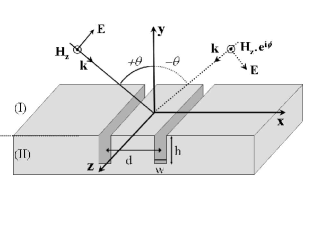
Figure 1: Geometrical configuration and parameters. Region (I) and (II) respectively corresponds to the region above and below the metallic surface. $\phi$ is the phase difference between the two incident waves described at the end of the paper.

where $I_{1}(x)$ (respectively $I_{2}(x)$) equal 1 in the interval $[(-w-d)/2,(w-d)/2]$ (resp. $[(d-w)/2,(d+w)/2]$) and zero elsewhere. $\alpha=[(1+Z)/(1-Z)]\Phi^{2}$, with $\Phi=e^{-ikh}$, $Z=1/\sqrt{\epsilon}$ is the surface impedance of the metal and $\epsilon$ its dielectric constant. The expression for $H_{z}^{(II)}$ assumes that the field is constant along $x$ within each groove, which is a good approximation in the limit where $w<<\lambda$ barbara1 ; barbara2 . To illustrate our results numerically, we have fixed $w=0.2$ $\mu m$, $h=1.5$ $\mu m$, and $d=0.5$ $\mu m$ all along the paper. The values of the complex dielectric constant $\epsilon(\lambda)$ are taken from handbook .
The unknown variables are the distribution $R(Q)$ and the field amplitudes $A_{1}$ and $A_{2}$ in the first and second groove respectively. A set of equations is obtained by applying the boundary conditions at the interface $y=0$ : $H_{z}^{(I)}=H_{z}^{(II)}$ at the mouth of each groove, and $\partial H_{z}^{(I)}/\partial y+ikZH_{z}^{(I)}=\partial H_{z}^{(II)}/\partial y+ikZH_{z}^{(II)}$ along the whole interface. After some elementary algebra (see barbara2 for detailed procedure), the vector ${\bf{A}}=(A_{1},A_{2})$ is related to the excitation vector ${\bf V}=(V_{1},V_{2})$ (null without the incoming wave), by the matricial relation ${\bf A}={\bf M}^{-1}{\bf V}$, where ${\bf M}$ is the $2\times 2$ symmetrical matrix which verifies $m_{11}=m_{22}$ with:

$${m_{11}} = {\left(1+\alpha\right)-\Gamma(1+Z)(1-\Phi^{2})\int_{-\infty}^{+\infty}{\frac{\sec^{2}\left(Qw/2\right)}{q+kZ}}dQ}$$

$${m_{12}} = {-\Gamma(1+Z)(1-\Phi^{2})\int_{-\infty}^{+\infty}{\frac{\sec^{2}\left(Qw/2\right)}{q+kZ}e^{iQd}dQ},}$$

where $\Gamma=w/\lambda$. The coordinates of the vector ${\bf V}$ are:

$${V_{1}} = {e^{-i\varphi}V_{0}}\quad\text{and}\quad{V_{2}}={e^{i\varphi}V_{0}}\quad\text{with:}$$

$${V_{0}} = {\frac{2\cos\theta}{\cos\theta+Z}\sec\left(k\sin(\theta)w/2\right)}$$

where we have introduced the angle $\varphi=kd\sin(\theta)/2$.
The matrix $\bf M$ has two eigenvalues $m_{\pm}=-i(1-\Phi^{2})e_{\pm}$ with respective eigenvectors ${\bf U}_{\pm}=(1,\pm 1)$ and:

$${e_{\pm}} = {\frac{1}{1-Z}\left(\cot(kh)-iZ\right)-2i\Gamma(1+Z)\times}$$

$$\times {\int_{0}^{+\infty}{(1\pm\cos\left(kdu\right))\frac{\sec^{2}(kwu/2)}{\sqrt{1-u^{2}}+Z}du}.}$$

We have made the variable change $Q=ku$ in the integrals. The solution of the problem is then:

$${A_{n=1,2}} = {\left[\frac{1}{e_{+}}+(-1)^{n}i\tan\varphi\frac{1}{e_{-}}\right]{\frac{i\cos(\varphi)}{1-\Phi^{2}}V_{0}}}$$

$${R(Q)} = {\frac{\cos\theta-Z}{\cos\theta+Z}\delta(Q-k\sin\theta)+\Gamma(1+Z)(1-\Phi^{2})\times}$$ (1)

$$\times {(e^{iQd/2}A_{1}+e^{-iQd/2}A_{2})\frac{\sec(Qw/2)}{q+kZ}}.$$

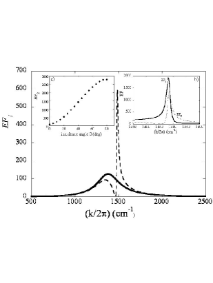
Figure 2: $EF_{1}$ of the cavity centered at $x=-d/2$ calculated for $\theta=0^{\circ}$ (full line) and $\theta=30^{\circ}$ (dotted line) as a function of the wavenumber. Inset a) represents the behavior of $EF_{2}$ (cavity centered at $x=+d/2$), as a function of the incidence angle $\theta$ and at 1484 $cm^{-1}$. Inset b) gives $EF_{1}$ and $EF_{2}$ of both cavities calculated for $50^{\circ}$.

At the sight of eq.(1), one can see that the system presents two electromagnetic resonances at $k=k_{\pm}$, which appear when $\Re(e_{+})=0$ and $\Re(e_{-})=0$, with lineshapes respectively governed by $\Im(e_{+})$ and $\Im(e_{-})$ ($\Re(x)$ and $\Im(x)$ being the real and imaginary parts of $x$). The fields in the cavities are always a linear combination of the two eigenvectors ${\bf A}\sim a_{-}{\bf U}_{-}+a_{+}{\bf U}_{+}$. However, when $k=k_{+}$ (respectively $k=k_{-}$), the vector ${\bf A}$ is almost collinear with ${\bf U_{+}}$ (resp. ${\bf U_{-}}$) as the amplitudes in the two cavities are dominated by the same (resp. the opposite) term. We will thus call the resonance occurring at $k=k_{-}$ the ($-$) antisymmetric mode and that occurring at $k=k_{+}$ the ($+$) symmetrical one. Contrary to the $(+)$ mode which always exists, the $(-)$ one only develops for $\theta\neq 0$ (see fig.2) as it vanishes at normal incidence with tan$\varphi=0$. Its bandwidth is much thinner than that of the symmetrical mode and its enhancement factor is much larger. The enhancement factor ($EF$), defined as $|E_{x}/E_{0}|^{2}$ where $E_{0}$ is the incident electric field, reflects the amount of stocked electromagnetic energy at the resonances. For convenience, we note $EF_{1}$ and $EF_{2}$ the enhancement factors calculated at the mouth of each cavity, i.e at $x=\pm d/2$ and $y=0$ where they are expressed as $EF_{n=1,2}=|A_{n=1,2}(1-\alpha)|^{2}$. The $EF$ of the $(-)$ mode, shown in the inset (a) of fig.2, increases with $\theta$ and its value can reach more than $10^{3}$ whereas that of the symmetrical mode stays at around $100$.
Another important point to highlight is that around the $(-)$ resonance, the fields in the two cavities are not strictly identical. Inset (b) of fig.2 displays the $EF$ at the mouth of each cavity close to $k=k_{-}$. At $1483$ $cm^{-1}$ the maximum of $EF_{1}$ is reached whereas the value of $EF_{2}$ is still low; at $1490$ $cm^{-1}$ $EF_{1}$ and $EF_{2}$ both take the same value. Around this mode, the system thus develops a very high sensitivity: with a very little variation of wavenumber (here less than one percent), the field ”jumps” from one cavity to the other. This behavior is qualitatively comparable to the ”unstable” behavior of hot spots observed on SERS active surfaces.

In the following, we consider the metal as being a perfect reflector, i.e $Z=0$. This approximation induces only small quantitative modifications and allows an analytical study which highly helps to clarify the physics of the problem. however, the presented numerical results are obtained without this approximation, i.e using the finite value of $\epsilon(\lambda)$. We first compare the two grooves system to the one where there is only one groove centered at $x=0$. In this case, the amplitude of the field $A_{0}$ in the unique cavity is given by $A_{0}=i\left[1-\Phi^{2}\right]^{-1}V_{0}/e$, with :

$$e=\cot(kh)-2i\Gamma\int_{0}^{+\infty}{\frac{\sec^{2}(kwu/2)}{\sqrt{1-u^{2}}}du}.$$

The resonance of this cavity occurs at $k=k_{0}=\omega_{0}/c$ for which $\Re(e)=0$. Close to $k_{0}$, the field $A_{0}$ can be expanded around $\omega_{0}$ as:

$$A_{0}\approx\frac{C_{0}}{\omega_{0}-\omega-i\gamma_{0}/2},$$

with $C_{0}\approx icV_{0}/2h$, and where we have taken advantage of the fact that at the resonance $k_{0}h\approx\pi/2$ barbara2 . This equation is typical of a forced oscillator and, as the electric field inside the cavity is proportional to $A_{0}$, indicates that the cavity behaves as a forced oscillating dipole with a radiation damping $\gamma_{0}=2w\omega_{0}^{2}/\pi c$ and an effective electromagnetic radius $r_{0}=2w/\pi$. The effective dipolar momentum, parallel to the interface, takes its maximum at the mouth of the groove and decreases along the vertical walls. The maximum of intensity at $\omega=\omega_{0}$ is $|A_{0}|^{2}\approx 4/(k_{0}w)^{2}$, typically of order 100 for our geometrical parameters. We now expand, in the same manner, the values of $e_{\pm}$ around the same $k_{0}$ for the two groove system. We easily get:

$${e_{+}} \approx {\left(\omega_{+}-\omega-i\gamma_{+}/2\right)h/c}$$ (2)

$${e_{-}} \approx {\left(\omega_{-}-\omega-i\gamma_{-}/2\right)h/c,}$$

with ${\omega_{\pm}}={\omega_{0}\mp\Delta}$, ${\gamma_{+}}={2\gamma_{0}}$ and ${\gamma_{-}}={\gamma_{0}\left(k_{0}d/2\right)^{2}}$. The shift $\Delta$, of the order of $\gamma_{0}\ll\omega_{0}$, is:

$$\Delta=\frac{\gamma_{0}}{\pi}\int_{1}^{+\infty}{\frac{\cos\left(k_{0}du\right)\sec^{2}\left(k_{0}wu/2\right)}{\sqrt{u^{2}-1}}du}$$ (3)

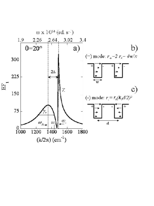
Figure 3: $EF_{1}$ calculated for $\theta=20^{\circ}$ showing the resonances $(+)$ and $(-)$ characterized by their eigenfrequencies $\omega_{\pm}$, located on both sides of the frequency resonance $\omega_{0}$ of a unique cavity, and their bandwidth $\gamma_{\pm}$ (a). Right part schematically represents the in-phase coupling of the $(+)$ mode (b) and the anti-phase coupling of the $(-)$ mode (c) and their corresponding equivalent dipole.

Eq. (2, 3) confirm our numerical observation as they show that the width of the $(-)$ mode, driven by $\gamma_{-}$, is much lower than that of the $(+)$ mode, driven by $\gamma_{+}$, owing to the small factor $(k_{0}d)^{2}$ (and recalling our sub-wavelength coupling hypothesis : $\lambda_{0}>>d$). A physical image of these resonances can be given noticing that our results are completely similar to those obtained by Lyuboshitzlyuboshitz for two near-field coupled oscillating dipoles. Our resonances thus arise from the near-field coupling of two identical grooves, individually resonating at $\omega_{0}$. The symmetrical $(+)$ mode corresponds to the in-phase oscillation of each cavity whereas the second one corresponds to an anti-phase oscillation. The distribution of electric field in the cavities for each mode is sketched in fig.3. As a consequence of this coupling, the $(+)$ mode has a strong dipolar character with an effective dipolar moment close to twice that of a unique cavity and a large electromagnetic radius $r_{+}=2r_{0}$. On the opposite, the $(-)$ mode has an effective dipolar moment almost null, with a much smaller electromagnetic radius $r_{-}=r_{0}(k_{0}d/2)^{2}$, and its radiation pattern is essentially that of a quadripole. This explains why this mode is weakly radiative and with an extremely narrow lineshape, very different from the width of the in-phase mode.
Searching for the location of the maximum of the field in each cavity around the $(-)$ mode, ones gets for non zero $\theta$:

$$\omega_{max.}^{n=1,2} \approx \omega_{-}-\frac{(-1)^{n}\left(\frac{k_{0}d}{2}\right)^{3}\gamma_{0}}{4\sin\theta\left(1+\left(\frac{2\Delta}{\gamma_{0}}\right)^{2}\right)}+O((k_{0}d)^{4})$$

$$|A_{max}|^{2} \approx \frac{16\sin^{2}\theta}{(k_{0}w)^{2}(k_{0}d)^{2}},$$

where $|A_{max}|^{2}$ is proportional to the intensity of the field in both cavities at $\omega_{max}$. The two maxima $\omega_{max}^{1}$ and $\omega_{max}^{2}$ are separated by a very small frequency difference of the order of $(k_{0}d)^{3}\gamma_{0}$, which, together with the narrow lineshape of the resonance, explains why the profile of the field strongly varies in this region. The magnitude of $|A_{max}|^{2}$ requires some comment. Indeed, for an usual oscillator with damping $\gamma$, the maximum of intensity of the oscillation scales as $\gamma^{-2}$, so that $|A_{max}|^{2}$ should scale as $\gamma_{-}^{-2}\sim(k_{0}d)^{-4}$ instead of $(k_{0}d)^{-2}$. The field intensity of the $(+)$ mode scales, as expected, as $\gamma_{+}^{-2}$ (eq. 1). The reason for that is that the ($+$) and $(-)$ modes are not sensitive to the same parts of the incident electric field. Since $d/\lambda\ll 1$, the latter can express at interface as $E_{0}(1+ikx)$ at the scale of our two-grooves system. The even term corresponding to the mean value of the field excites the $(+)$ mode and the odd one, corresponding to the local variations of the field, excites the $(-)$ mode. This mode is thus sensitive to an ”effective” field of intensity $\sim E_{0}^{2}(k_{0}d)^{2}$ at the mouth of the grooves, whereas the $(+)$ mode is excited by an effective field of intensity $E_{0}^{2}$. This is the origin of the lost of a factor $(k_{0}d)^{-2}$ in the intensities of the mode $(-)$. The latter results from a strong resonator, but excited by a very weak effective field.

We now take advantage of our understanding to control - from far field - the light localization in the cavity of our choice, or in both. To do so, we introduce a new free parameter by sending a second incident plane wave, at the same frequency, with an incidence angle $-\theta$, and with a phase difference $\phi$ with respect to the first incident wave (fig.1). Changing $\phi$, we can control the incident effective fields respectively exciting one mode or the other. Different states, that we code as : $(1,1)$, $(1,-1)$, $(1,0)$ and $(0,-1)$ can be achieved. The first two, $(1,1)$ and $(1,-1)$ respectively correspond to the case where only the pure $(+)$ or only the pure $(-)$ resonances are excited. The cavities are then completely in-phase or in anti-phase. The two other ones correspond to cases where one of the cavities is lit (cavity 1 for $(1,0)$, and cavity 2 for $(0,-1)$). As $\phi$ is a parameter easy to modify, for instance changing the optical path, we can control in straightforward manner the field localization.
With two incoming waves, the field becomes:

$$H_{inc.}=\left[e^{ik\sin\theta x}+e^{i\left(\phi-k\sin\theta x\right)}\right]e^{-ik\cos\theta y},$$

and the solution for each cavity can be written as:

$$A_{n=1,2}\sim\frac{\cos(\phi/2)}{e_{+}}+(-1)^{n}\tan\varphi\frac{\sin(\phi/2)}{e_{-}}\\$$ (4)

where we did not write explicitly some unimportant prefactor common to both cavities. From these equations, it is easy to see that for $\phi=\phi_{(1,1)}=0$, one gets $A_{1}=A_{2}\sim 1/e_{+}$, so that at $k=k_{+}$ we have the pure $(+)$ resonance. In the same manner, the pure $(-)$ resonance can be excited at $k=k_{-}$ when $\phi=\phi_{(1,-1)}=\pi$ where $A_{1}=-A_{2}\sim-\tan\varphi/e_{-}$. This last state presents an extremely high $EF\sim 10^{4}$ at $\theta=80^{\circ}$.
More subtle is the possibility to control the extinction of the field in only one of the cavities (of our choice) while the other one is resonating.

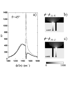
Figure 4: $EF_{1}$ and $EF_{2}$ spectra at $\theta=45^{\circ}$ for two incoming waves (a) and related mappings of the electric field amplitude $E_{x}$ (b, c) at 1490 $cm^{-1}$. For $\phi=\phi_{(1,0)}$ the first cavity is lit, $EF_{1}$ is the dotted line, and the second cavity is extinguished, $EF_{2}$ is the full line. For $\phi=\phi_{(0,-1)}$ it is the opposite.

Eq.(4) shows that this can be achieved provided that $\cot\phi/2=\pm(e_{+}/e_{-})\tan\varphi$, the sign $"+"$ corresponding to the $(0,-1)$ state and the $"-"$ sign to the $(1,0)$ state. This condition can be satisfied (since the function $\cot(x)$ can vary from $-\infty$ to $+\infty$), provided that $e_{+}/e_{-}$ is real. This is obtained for $\omega\approx\omega_{-}+2\Delta(\gamma_{-}/\gamma_{+})$, which is very close to $\omega_{-}$. Figure 4 represents the $EF$ of both cavities either choosing $\phi=\phi_{(1,0)}$ or $\phi=\phi_{(0,-1)}$, together with the related mappings of the electric field amplitude $E_{x}$. These show how the field can be strongly localized in only one of the cavity, while the second one is completely extinguished and this, even though the cavities are identical and separated by a sub-wavelength distance.
In conclusion, we have demonstrated that the near-field coupling of two metallic resonating cavities leads to a resonance with an extremely thin spectral width, which can localize very intense fields. This could be a key point in the understanding of the SERS, as the described physics should remain valid in the visible region, except for a scaling factor. Finally, we proposed a simple way to control the near-field of each cavity, enabling this system to act as a sub-wavelength optical switch simply operated from the far-field.