Comparison of free energy methods for molecular systems

Abstract

We present a detailed comparison of computational efficiency and precision for several free energy difference ($\Delta F$) methods. The analysis includes both equilibrium and non-equilibrium approaches, and distinguishes between uni-directional and bi-directional methodologies. We are primarily interested in comparing two recently proposed approaches, adaptive integration and single-ensemble path sampling, to more established methodologies. As test cases, we study relative solvation free energies, of large changes to the size or charge of a Lennard-Jones particle in explicit water. The results show that, for the systems used in this study, both adaptive integration and path sampling offer unique advantages over the more traditional approaches. Specifically, adaptive integration is found to provide very precise long-simulation $\Delta F$ estimates as compared to other methods used in this report, while also offering rapid estimation of $\Delta F$. The results demonstrate that the adaptive integration approach is the best overall method for the systems studied here. The single-ensemble path sampling approach is found to be superior to ordinary Jarzynski averaging for the uni-directional, “fast-growth” non-equilibrium case. Closer examination of the path sampling approach on a two-dimensional system suggests it may be the overall method of choice when conformational sampling barriers are high. However, it appears that the free energy landscapes for the systems used in this study have rather modest configurational sampling barriers.

I Introduction

Free energy difference ($\Delta F$) calculations are useful for a wide variety of applications, including drug design Jorgensen (2004); Sotriffer et al. (2003), solubility of small molecules Pitera and van Gunsteren (2001); Grossfield et al. (2003), and protein/ligand binding affinities Singh et al. (1994); Oostenbrink et al. (2000); Fujitani et al. (2005). Due to the high computational cost of $\Delta F$ calculations, it is of interest to carefully compare the efficiencies of the various approaches.

We are particularly interested in assessing recently proposed methods Fasnacht et al. (2004); Ytreberg and Zuckerman (2004a) in comparison to established techniques. Thus, the purpose of this study is to provide a careful comparison of the efficiency and precision of several $\Delta F$ methods. We seek to answer two important questions: (i) Given a fixed amount of computational time ($10^{6}$ dynamics steps, in this study), which method estimates the correct value of $\Delta F$ with the greatest precision? (ii) Which $\Delta F$ approach can obtain a “reasonable” estimate of $\Delta F$ in the least amount of computational time?

Free energy difference methods can be classified as either equilibrium or non-equilibrium. Equilibrium approaches include multi-stage free energy perturbation Zwanzig (1954), thermodynamic integration Kirkwood (1935); Straatsma and McCammon (1991), Bennett analysis Bennett (1976); Shirts and Pande (2005) and weighted histogram analysis Kumar et al. (1992). The common theme in these approaches is that sufficiently long equilibrium simulations are performed at each intermediate stage of the free energy calculation. Equilibrium methods are in wide use and are known to provide accurate results; however, the computational cost can be large due the simulation time needed to attain equilibrium at each intermediate stage. A host of non-equilibrium methods have recently been applied to various molecular systems, largely due to Jarzynski’s remarkable equality Jarzynski (1997a); Crooks (2000). Non-equilibrium methods have the potential to provide very rapid estimates of $\Delta F$, but can suffer from significant bias Ytreberg and Zuckerman (2004b); Zuckerman and Woolf (2002); Hummer (2001).

In this report we present results using both equilibrium and non-equilibrium approaches—as well as uni-directional and bi-directional methodology. Specifically, we compare: (i) adaptive integration Fasnacht et al. (2004); (ii) thermodynamic integration Kirkwood (1935); (iii) single-ensemble path sampling of non-equilibrium work values using Jarzynski’s uni-directional averaging Ytreberg and Zuckerman (2004a); (iv) single-ensemble path sampling using Bennett’s bi-directional formalism; (v) Jarzynski averaging of non-equilibrium work values Jarzynski (1997a, b); (vi) Bennett analysis of non-equilibrium work values Crooks (2000); Shirts et al. (2003a); (vii) equilibrium Bennett analysis Bennett (1976); Shirts and Pande (2005); and (viii) multi-stage free energy perturbation Zwanzig (1954). We also compare the free energy profiles, which determines the potential of mean force, for adaptive integration and thermodynamic integration.

Generally, one is interested in the free energy difference ($\Delta F=F_{1}-F_{0}$) between two states or systems of interest denoted by potential energy functions $U_{0}(\vec{x})$ and $U_{1}(\vec{x})$, where $\vec{x}$ is the full set of configurational coordinates. $\Delta F$ can be written in terms of the partition functions for each state

$$\Delta F=-k_{B}T\ln\Bigg{(}\frac{Z\big{[}U_{1}(\vec{x})\big{]}}{Z\big{[}U_{0}(\vec{x})\big{]}}\Bigg{)},$$ (1)

where $k_{B}$ is the Boltzmann constant, $T$ is the system temperature, and $Z[U(\vec{x})]=\int d\vec{x}\exp[-U(\vec{x})/k_{B}T]$. Because the overlap between the configurations in $U_{0}$ and $U_{1}$ may be poor, a “path” connecting $U_{0}$ and $U_{1}$ is typically created. In our notation, the path will be parameterized using the variable $\lambda$, with $0\leq\lambda\leq 1$.

II Equilibrium free energy calculation

Equilibrium free energy methodologies share the common strategy of generating equilibrium ensembles of configurations at multiple values of the scaling parameter $\lambda$. In the current study we investigate thermodynamic integration Kirkwood (1935), adaptive integration Fasnacht et al. (2004), multi-stage free energy perturbation Zwanzig (1954), and multi-stage equilibrium Bennett analysis Bennett (1976). We performed separate equilibrium simulations at successive values of $\lambda$, and then estimated $\Delta F$ using free energy perturbation, Bennett averaging, and thermodynamic integration on the resulting ensemble of configurations (detailed in Sec. IV).

II.1 Thermodynamic integration

Thermodynamic integration (TI) is probably the most common fully equilibrium $\Delta F$ approach. In TI, equilibrium simulations are performed at multiple values of $\lambda$. Then, $\Delta F$ is found by approximating the integral Kirkwood (1935),

$$\Delta F=\int_{\lambda=0}^{1}d\lambda\left<\frac{\partial U_{\lambda}({\vec{x}})}{\partial\lambda}\right>_{\lambda},$$ (2)

where the functional form for $U_{\lambda}(\vec{x})$ depends upon the scaling methodology and will be discussed in detail in Sec. IV. The notation $\langle...\rangle_{\lambda}$ indicates an ensemble average at a particular value of $\lambda$. In addition to the possibility of inadequate equilibrium sampling at each $\lambda$ value, error arises in TI from the fact that only a finite number of $\lambda$ values can be simulated, and thus the integral must be approximated by a sum Shirts and Pande (2005). Thermodynamic integration can provide very accurate $\Delta F$ calculations, but can also be computationally expensive due to the equilibrium sampling required at each $\lambda$ value Boresch et al. (2003); Mordasini and McCammon (2000); Shirts et al. (2003b); Lybrand et al. (1985).

II.2 Adaptive integration

The adaptive integration method (AIM), detailed in Ref. Fasnacht et al., 2004, seeks to estimate the same integral as that of TI; namely Eq. (2) (see also discussions in Refs. Marinari and Parisi, 1992; Tidor, 1993; Kong and Brooks, 1996; Wang and Landau, 2001; Earl and Deem, 2005). However, in addition to fixed-$\lambda$ equilibrium sampling, the AIM approach uses a Metropolis Monte Carlo procedure to generate equilibrium ensembles for the set of $\lambda$ values. The $\lambda$-sampling is done by attempting Monte Carlo moves that change the value of $\lambda$ during the simulation. The probability of accepting a change from the old value $\lambda_{o}$ to a new value $\lambda_{n}$ is

$$P_{\rm acc}(\lambda_{o}\rightarrow\lambda_{n})=$$

$$\min\left[1.0,e^{-\beta\bigl{(}U_{\lambda_{n}}(\vec{x})-U_{\lambda_{o}}(\vec{x})\bigr{)}}e^{+\beta\bigl{(}\delta\hat{F}(\lambda_{n})-\delta\hat{F}(\lambda_{o})\bigr{)}}\right],$$ (3)

where $\beta=1/k_{B}T$ and $\delta\hat{F}(\lambda_{i})$ is the current running free energy estimate obtained by numerically approximating the integral

$$\delta\hat{F}(\lambda_{i})=\int_{\lambda=0}^{i}d\lambda\left<\frac{\partial U_{\lambda}({\vec{x}})}{\partial\lambda}\right>_{\lambda}.$$ (4)

Between attempted Monte Carlo moves in $\lambda$, any canonical sampling scheme (e.g., molecular dynamics, Langevin dynamics, Monte Carlo) can be used to propagate the system at fixed $\lambda$. In this report, Langevin dynamics is used to sample configurations, and Monte Carlo moves in $\lambda$ are attempted after every time step.

It is important to note that, due to the use of the running estimate $\delta\hat{F}$ in Eq. (3), the AIM method satisfies detailed balance only asymptotically. In other words, once the $\Delta F$ estimate fully converges, the value of $\delta\hat{F}$ is correct, and detailed balance is satisfied Fasnacht et al. (2004); Earl and Deem (2005).

AIM is related to parallel tempering simulation Marinari and Parisi (1992), and has the associated advantage: equilibrium sampling of conformational space at one $\lambda$ value can assist sampling at other $\lambda$ values due to the frequent $\lambda$ moves. This is reminiscent of “$\lambda$ dynamics” simulation Tidor (1993); Kong and Brooks (1996), but contrasts with TI where only a single starting configuration is passed between $\lambda$ values.

An additional advantage of AIM over the other methods detailed in this report is that there is a simple, built-in, reliable, convergence criterion. Specifically, one can keep track of the population (number of simulation snapshots) at each value of $\lambda$. When the estimate for $\Delta F$ has converged, the population will be approximately uniform across all values of $\lambda$. If the population is not approximately uniform, then the simulation must be continued.

II.3 Free energy perturbation

In the free energy perturbation approach, one performs independent equilibrium simulations at each $\lambda$ value (like TI), then uses exponential averaging to determine the free energy difference between neighboring $\lambda$ values Zwanzig (1954)—these differences are then summed to obtain the total free energy difference. $\Delta F$ can be approximated for a path containing $n$ $\lambda$-values (including $\lambda=0$ and $\lambda=1$) using the “forward” estimate (FEPF)

$$\Delta F=-k_{B}T\sum_{i=0}^{n-1}\ln\Bigl{<}e^{-\beta(U_{\lambda_{i+1}}(\vec{x}_{i})-U_{\lambda_{i}}(\vec{x}_{i})}\Bigr{>}_{\lambda_{i}},$$ (5)

or the “reverse” estimate (FEPR)

$$\Delta F=+k_{B}T\sum_{i=0}^{n-1}\ln\Bigl{<}e^{-\beta(U_{\lambda_{i}}(\vec{x}_{i+1})-U_{\lambda_{i+1}}(\vec{x}_{i+1})}\Bigr{>}_{\lambda_{i+1}}.$$ (6)

A primary limitation of free energy perturbation is that the spacing between $\lambda$ values must be small enough that there is sufficient overlap between all pairs ($\lambda_{i},\;\lambda_{i+1}$) of configuration spaces.

II.4 Equilibrium Bennett estimation

It is also possible to use Bennett’s method to combine the information normally used for forward and reverse free energy perturbation. In this approach, one computes the free energy difference between successive $\lambda$ values $\delta F_{i}$ according to

$$\Bigg{<}\bigg{[}1+e^{\beta\big{(}U_{\lambda_{i+1}}(\vec{x}_{i})-U_{\lambda_{i}}(\vec{x}_{i})-\delta F_{i}\big{)}}\bigg{]}^{-1}\Bigg{>}_{\lambda_{i}}=$$

$$\Bigg{<}\bigg{[}1+e^{\beta\big{(}U_{\lambda_{i+1}}(\vec{x}_{i+1})-U_{\lambda_{i}}(\vec{x}_{i+1})+\delta F_{i}\big{)}}\bigg{]}^{-1}\Bigg{>}_{\lambda{i+1}}.$$ (7)

Then the sum of these $\delta F_{i}$ is the total free energy difference Bennett (1976);

$$\Delta F=\sum_{i=0}^{n-1}\delta F_{i}.$$ (8)

Studies have shown that using the Bennett method to evaluate free energy data is the most efficient manner to utilize two equilibrium ensembles Shirts and Pande (2005); Lu et al. (2003).

III Non-equilibrium free energy estimation

In non-equilibrium free energy approaches, the system is forced to switch to subsequent $\lambda$ values, whether or not equilibrium has been reached at the current $\lambda$ value. In this way, non-equilibrium paths are generated that connect $U_{0}$ and $U_{1}$. In the current study we use uni-directional Jarzynski averaging Jarzynski (1997a) and bi-directional Bennett averaging of Jarzynski-style work values Crooks (2000), as well as uni-directional Ytreberg and Zuckerman (2004a) and bi-directional averaging of path sampled work values.

III.1 Jarzynski averaging

For the Jarzynski method Jarzynski (1997a), one considers non-equilibrium paths that alternate between increments in $\lambda$ and “traditional” dynamics (e.g., Monte Carlo or molecular dynamics) in $\vec{x}$ at fixed $\lambda$ values. Thus, a path with $n$ $\lambda$-steps is given by

$${\bf Z}_{n}=\Bigl{\{}(\lambda_{0}=0,\vec{x}_{0}),(\lambda_{1},\vec{x}_{0}),(\lambda_{1},\vec{x}_{1}),(\lambda_{2},\vec{x}_{1}),$$

$$(\lambda_{2},\vec{x}_{2}),...,(\lambda_{n-1},\vec{x}_{n-1}),(\lambda_{n}=1,\vec{x}_{n-1})\Bigr{\}},$$ (9)

where it should be noted that increments (steps) from $\lambda_{i}$ to $\lambda_{i+1}$ are performed at a fixed conformation $\vec{x}_{i}$, and the initial $\vec{x}_{0}$ is drawn from the canonical $U_{0}$ distribution. For simplicity, Eq. (9) shows only a single dynamics step performed at each fixed $\lambda_{i}$, from $\vec{x}_{i-1}$ to $\vec{x}_{i}$; However, multiple steps may be implemented, as below (Sec. V). A “forward” work value is thus given by

$$W_{\rm f}({\bf Z}_{n})=\sum_{i=0}^{n-1}\Bigl{[}U_{\lambda_{i+1}}(\vec{x}_{i})-U_{\lambda_{i}}(\vec{x}_{i})\Bigr{]}.$$ (10)

By generating multiple paths (and thus work values) it is possible to estimate $\Delta F$ via Jarzynski’s equality Jarzynski (1997a)

$$\Delta F=-k_{B}T\ln\left<e^{-\beta W_{\rm f}}\right>_{0},$$ (11)

where the $\left<...\right>_{0}$ represents an average over forward work values $W_{\rm f}$ generated by starting the system at $U_{0}$ and ending at $U_{1}$. A similar expression can be written for the situation when work values are generated by switching from $U_{1}$ to $U_{0}$. This approach is “uni-directional” since only work values from either forward or reverse data are used.

Perhaps the most remarkable aspect of Eq. (11) is that it is valid for arbitrary switching speed. However, in practice, the $\Delta F$ estimates are very sensitive to the distribution of work values, which in turn is largely dependent on the switching speed. If the distribution of work values is non-Gaussian and the width is large ($\sigma_{W}\gg k_{B}T$), then the $\Delta F$ estimate can be heavily biased Hummer (2001); Gore et al. (2003); Zuckerman and Woolf (2002); Ytreberg and Zuckerman (2004b). Consistent with results in this report (Sec. V), other efficiency studies Hummer (2001); Crooks (2000) have suggested that the optimal efficiency for uni-directional Jarzynski averaging is when the switching speed is slow enough that $\sigma_{W}\approx 1\;k_{B}T$.

III.2 Bennett averaging of Jarzynski work values

Due to the bias introduced in using uni-directional Jarzynski averaging, it is useful to consider a method where both forward and reverse work values are utilized. It has been shown that the most efficient use of bi-directional data is via Bennett’s method Crooks (2000); Shirts et al. (2003a),

$$\sum_{N_{\rm f}}\bigg{[}1+e^{\beta\big{(}\eta+W_{\rm f}-\Delta F\big{)}}\bigg{]}^{-1}=\sum_{N_{\rm r}}\bigg{[}1+e^{\beta\big{(}-\eta+W_{\rm r}+\Delta F\big{)}}\bigg{]}^{-1},$$ (12)

where $\eta=k_{B}T\ln\left(N_{\rm f}/N_{\rm r}\right)$ allows for differing number of forward ($N_{\rm f}$) and reverse ($N_{\rm r}$) work values. Equation (12) must be solved iteratively since $\Delta F$ appears in the sum on both sides of the equation.

III.3 Single-ensemble path sampling

Single-ensemble path sampling (SEPS) is a non-equilibrium approach that seeks to generate “important” paths more frequently Sun (2003); Atilgan and Sun (2004); Athènes (2002, 2004); Adjanor and Athènes (2005); Ytreberg and Zuckerman (2004a). The method uses importance sampling to generate paths (and thus work values) according to an arbitrary distribution $D$, here chosen as Ytreberg and Zuckerman (2004a)

$$D({\bf Z}_{n})=Q({\bf Z}_{n})\;e^{-\frac{1}{2}\beta W({\bf Z}_{n})},$$ (13)

where $Q({\bf Z}_{n})$ is proportional to the probability of occurrence of an ordinary Jarzynski path, and is given below. With this choice of $D$ the free energy is estimated via (compare to Refs. Sun, 2003; Atilgan and Sun, 2004; Athènes, 2002, 2004; Adjanor and Athènes, 2005)

$$\Delta F=-k_{B}T\ln\bigg{[}{\sum}^{D}e^{-\frac{1}{2}\beta W_{\rm f}}\bigg{/}{\sum}^{D}e^{+\frac{1}{2}\beta W_{\rm f}}\bigg{]},$$ (14)

where the ${\sum}^{D}$ is a reminder that the work values used in the sum must be generated according to the distribution in Eq. (13). Since forward work values, $W_{f}$ are utilized in Eq. (14), the paths must start in $U_{0}$ and end in $U_{1}$. A similar expression can be written for reverse work values $W_{\rm r}$.

To generate work values according to the distribution $D$, path sampling must be used Pratt (1986); Bolhuis et al. (2002); Hummer (2004); Sun (2003); Atilgan and Sun (2004); Athènes (2002, 2004); Adjanor and Athènes (2005); Ytreberg and Zuckerman (2004a). In path sampling, entire paths are generated and then accepted or rejected according to a suitable Monte Carlo criteria. In general, the probability of accepting a trial path with $n$ $\lambda$-steps (${\bf Z}_{n}^{\prime}$ with work value $W^{\prime}$) that was generated from an existing path (${\bf Z}_{n}$ with work value $W$) is given by

$$P_{\rm acc}^{{\bf Z}_{n}\rightarrow{\bf Z}_{n}^{\prime}}=\min\Bigg{[}1,\frac{Q({\bf Z}_{n}^{\prime})\;P_{\rm gen}^{{\bf Z}_{n}^{\prime}\rightarrow{\bf Z}_{n}}\;e^{-\frac{1}{2}\beta W^{\prime}}}{Q({\bf Z}_{n})\;P_{\rm gen}^{{\bf Z}_{n}\rightarrow{\bf Z}_{n}^{\prime}}\;e^{-\frac{1}{2}\beta W}}\Bigg{]},$$ (15)

where $P_{\rm gen}^{X\rightarrow Y}$ is the conditional probability of generating a trial path $Y$ from existing path $X$.

For this study, we generate trial paths by randomly choosing a “shoot” point $\lambda_{s}$ along an existing path (compare to Refs. Bolhuis et al., 2002; Dellago et al., 1999; Dellago et al., 1998a). Then, Langevin dynamics is used to propagate the system from $\lambda_{s}\rightarrow 0$ (backward segment), followed by $\lambda_{s}\rightarrow 1$ (forward segment). Before running the backward segment, the velocities at the shoot point must be reversed and then ordinary Langevin dynamics are used to propagate the system Bolhuis et al. (2002). Once the trial path is complete, all the velocities for the backward segment are reversed. Since the stochastic Langevin algorithm is employed in the simulation, it is not necessary to perturb the configurational coordinates at the shoot point to obtain a trial path that differs from the existing path.

The above recipe for generating trial paths leads to the following statistical weights for the existing $Q({\bf Z}_{n})$ and trial $Q({\bf Z}_{n}^{\prime})$ paths

$$Q({\bf Z}_{n})=e^{-\beta U_{0}(\vec{x}_{0})}\;\prod_{i=0}^{n-1}p(\vec{x}_{i}\rightarrow\vec{x}_{i+1}),$$

$$Q({\bf Z}_{n}^{\prime})=e^{-\beta U_{0}(\vec{x}_{0}^{\prime})}\;\prod_{i=0}^{n-1}p(\vec{x}_{i}^{\prime}\rightarrow\vec{x}_{i+1}^{\prime}),$$ (16)

where $p(\vec{x}_{i}\rightarrow\vec{x}_{i+1})$ is the the transition probability for taking a dynamics step from configuration $\vec{x}_{i}$ to $\vec{x}_{i+1}$ Dellago et al. (1998a). We have assumed for simplicity that only one dynamics step is taken at each value of $\lambda$; however, the approach allows for multiple steps. The corresponding generating probabilities for the existing and trial paths are given by

$$P_{\rm gen}^{{\bf Z}_{n}\rightarrow{\bf Z}_{n}^{\prime}}=$$

$$p_{\rm choose}\;p_{\rm perturb}\;\prod_{i=s}^{n-1}p(\vec{x}_{i}^{\prime}\rightarrow\vec{x}_{i+1}^{\prime})\;\prod_{i=0}^{s-1}\bar{p}(\vec{x}_{i+1}^{\prime}\rightarrow\vec{x}_{i}^{\prime}),$$

$$P_{\rm gen}^{{\bf Z}_{n}^{\prime}\rightarrow{\bf Z}_{n}}=$$

$$p_{\rm choose}^{\prime}\;p_{\rm perturb}^{\prime}\;\prod_{i=s}^{n-1}p(\vec{x}_{i}\rightarrow\vec{x}_{i+1})\;\prod_{i=0}^{s-1}\bar{p}(\vec{x}_{i+1}\rightarrow\vec{x}_{i}),$$ (17)

where $\bar{p}(\vec{x}_{i+1}\rightarrow\vec{x}_{i})$ is the transition probability of taking a backward step from $\vec{x}_{i+1}$ to $\vec{x}_{i}$. The “bar” notation is a reminder that the velocities are reversed for these segments. The probability of choosing a particular shoot point $\lambda_{s}$ is denoted by $p_{\rm choose}$, and the probability of a particular perturbation to the configurational coordinates at the shoot point is given by $p_{\rm perturb}$.

Since we have chosen not to perturb the configurational coordinates at the shoot point, and any value of $\lambda$ along the path is equally likely to be chosen as the shoot point, then $p_{\rm perturb}=p_{\rm perturb}^{\prime}$ and $p_{\rm choose}=p_{\rm choose}^{\prime}$. In addition, since the transition probabilities obey detailed balance and preserve the canonical distribution then Dellago et al. (1998b)

$$\bar{p}(\vec{x}_{i+1}\rightarrow\vec{x}_{i})=p(\vec{x}_{i}\rightarrow\vec{x}_{i+1})\;e^{-\beta\big{(}U_{\lambda_{i+1}}(\vec{x}_{i})-U_{\lambda_{i+1}}(\vec{x}_{i+1})\big{)}}.$$ (18)

Inserting Eqs. (16), (17) and (18) into Eq. (15) gives the acceptance criterion for trial paths (compare to Eq. (45) in Ref. Adjanor and Athènes, 2005)

$$P_{\rm acc}^{{\bf Z}_{n}\rightarrow{\bf Z}_{n}^{\prime}}=\min\Bigg{[}1,{e^{-\beta\big{(}\delta W-\delta W^{\prime}+\frac{1}{2}(W^{\prime}-W)\big{)}}}\Bigg{]},$$ (19)

where $\delta W$ is defined as the work accumulated up to the shoot point for the existing path

$$\delta W=\sum_{i=0}^{s-1}\Bigl{[}U_{\lambda_{i+1}}(\vec{x}_{i})-U_{\lambda_{i}}(\vec{x}_{i})\Bigr{]}.$$ (20)

and $\delta W^{\prime}$ is the equivalent quantity for the trial path. Note that Eq. (19) is independent of the details of the fixed-$\lambda$ dynamics.

To clarify ambiguities in our original presentation of the SEPS approach Ytreberg and Zuckerman (2004a), we also give details for applying it using overdamped Langevin dynamics (i.e., Brownian dynamics). In Ref. Ytreberg and Zuckerman, 2004a, backward segments were generated using ordinary dynamics with negative forces, i.e., to be very clear, the force was taken to be identical to the physical force, but opposite in sign. Thus, the transition probabilities for forward and backward steps are approximately equal

$$\bar{p}(\vec{x}_{i+1}\rightarrow\vec{x}_{i})\approx p(\vec{x}_{i}\rightarrow\vec{x}_{i+1}).$$

(Brownian dynamics) (21)

Equality occurs when the forces at $\vec{x}_{i}$ and $\vec{x}_{i+1}$ are identical. The acceptance criterion becomes

$$P_{\rm acc}^{{\bf Z}_{n}\rightarrow{\bf Z}_{n}^{\prime}}=\min\Bigg{[}1,{e^{-\beta\big{(}\frac{1}{2}(W^{\prime}-W)+U_{0}(\vec{x}_{0}^{\prime})-U_{0}(\vec{x}_{0})\big{)}}}\Bigg{]}.$$

(Brownian dynamics) (22)

Therefore, the criticism raised in a recent paper Adjanor and Athènes (2005) is incorrect.

III.4 Bennett averaging of path sampled work values

The use of bi-directional data is worth considering for the SEPS method, just as it was for ordinary non-equilibrium Jarzynski work values. Generalizing Bennett’s method to include the work values sampled from $D$ gives

$${\sum_{N_{\rm f}}}^{D}\frac{e^{+\frac{1}{2}\beta W_{\rm f}}}{1+e^{\beta\big{(}\eta+W_{\rm f}-\Delta F\big{)}}}\bigg{[}{\sum_{N_{\rm f}}}^{D}e^{+\frac{1}{2}\beta W_{\rm f}}\bigg{]}^{-1}=$$

$${\sum_{N_{\rm r}}}^{D}\frac{e^{+\frac{1}{2}\beta W_{\rm r}}}{1+e^{\beta\big{(}-\eta+W_{\rm r}+\Delta F\big{)}}}\bigg{[}{\sum_{N_{\rm r}}}^{D}e^{+\frac{1}{2}\beta W_{\rm r}}\bigg{]}^{-1}.$$ (23)

Thus, to obtain a Bennett-averaged estimate for $\Delta F$, the path sampling algorithm is applied to generate an ensemble of paths going from $U_{0}$ to $U_{1}$ ($W_{\rm f}$, forward) and also for $U_{1}$ to $U_{0}$ ($W_{\rm r}$, reverse). Then, Eq. (23) is applied to the data.

IV Simulation details

To test the efficiency and precision of each method detailed above we use two relative solvation free energy calculations. One involves a large change in the van der Waals radius of a neutral particle in explicit solvent (“growing”), and the other is a large change in the charge of the particle while keeping the size fixed (“charging”).

The system used in both cases consists of a single Lennard-Jones particle in a 24.93 Å box of 500 TIP3P water molecules. For all simulations, the molecular simulation package TINKER 4.2 was used Ponder and Richard (1987). The temperature of the system was maintained at 300.0 K using Langevin dynamics with a friction coefficient of 5.0 $\rm ps^{-1}$. RATTLE was used to constrain all hydrogens to their ideal lengths Andersen (1983), allowing a 2.0 fs time step. A cutoff of 12.465 Å was chosen for electrostatic and van-der-Waals interactions with a smoothing function implemented from 10.465 to 12.465 Å. It is expected that the use of cutoffs will introduce systematic errors into the $\Delta F$ calculation, however, in this report we are only interested in comparing $\Delta F$ methodologies—we do not compare our results to experimental data.

For the first test case, a neutral Lennard-Jones particle was “grown” from 2.126452 Å to 6.715999 Å. The sizes were chosen to be that of lithium and cesium from the OPLS-AA forcefield Jorgensen et al. (1996). In the second test case, the Lennard-Jones particle remains at a fixed size of 2.126452 Å, but the charge is changed from -e/2 to +e/2. For each test case, and each $\Delta F$ method, the system was initially equilibrated for 100 ps ($5\times 10^{4}$ dynamics steps). The initial equilibration is not included in the total computational time listed in the results, however, since every method was given identical initial equilibration times, the efficiency analysis is fair.

The $\lambda$-scaling (i.e., the form of the hybrid potential $U_{\lambda}$) used for all $\Delta F$ methods in this study was chosen to be the default implementation within the TINKER package Ponder and Richard (1987). If a particle’s charge is varied from $q_{0}$ to $q_{1}$, the hybrid potential is simply the regular potential energy calculated using a hybrid charge of

$$q_{\lambda}=\lambda q_{1}+(1-\lambda)q_{0}.$$ (24)

Similarly, if a particle has a change in the van der Waals parameters $r,\;\epsilon$ the hybrid parameters are given by

$$r_{\lambda}=\lambda r_{1}+(1-\lambda)r_{0},$$

$$\epsilon_{\lambda}=\lambda\epsilon_{1}+(1-\lambda)\epsilon_{0}.$$ (25)

The free energy slope as a function of $\lambda$ for both the growing and charging test cases are shown in Figs. 1 and 3. The smoothness of both plots suggests that a more sophisticated $\lambda$-scaling is not necessary for this study. If, for example, we had chosen to grow a particle from nothing, then it is likely that a different scaling would be needed (such as in Refs. Kong and Brooks, 1996; Yang et al., 2004; Shirts et al., 2003b; Shirts and Pande, 2005).

IV.1 Thermodynamic integration calculations

For thermodynamic integration (TI), equilibrium simulations were performed at each value of $\lambda$. An equal amount of simulation time was devoted to each of 21 equally spaced values of $\lambda=0.0,0.05,0.1,...,0.9,0.95,1.0$. Averages of the slope ${\rm d}F/{\rm d}\lambda=\langle{\rm d}U/{\rm d}\lambda\rangle_{\lambda}$, shown in Figs. 1 and 3, were collected for each value of $\lambda$. The first 50% of the slope data were discarded for equilibration. Finally, the data were used to estimate the integral in Eq. (2) using the trapezoidal rule. Note that higher order integration schemes were also attempted, but did not change the results, suggesting that the curves in Figs. 1 and 3 are smooth enough that high order integration schemes are not needed for this report. Also, the percentage of data that was discarded for equilibration was varied from 25-75% with no significant changes to the results.

IV.2 Adaptive integration calculations

Adaptive integration (AIM) results were obtained by collecting the slope of the free energy ${\rm d}F/{\rm d}\lambda=\langle{\rm d}U/{\rm d}\lambda\rangle_{\lambda}$, by starting the simulation from an equilibrated configuration at $\lambda=0$ and performing one dynamics step. Immediately following the single step, a Monte Carlo move in $\lambda$ was attempted, which was accepted with probability given by Eq. (3). The pattern of one dynamics step followed by one Monte Carlo trial move was repeated until a total of $10^{6}$ dynamics steps (and thus $10^{6}$ Monte Carlo attempts) had been performed. The same $\lambda$ values used in TI are also used for AIM, thus $\lambda=0.0,0.05,0.1,...,0.9,0.95,1.0$ are the only allowed values. For this report Monte Carlo moves were attempted between neighboring values of $\lambda$ only, i.e., a move from $\lambda$=0.35 to 0.4 or 0.3 may be attempted but not to 0.45. Also, all $\delta\hat{F}(\lambda_{i})$ values of Eq. (4) were initially set to zero. The estimate of the free energy was obtained by numerically approximating the integral in Eq. (2) using the trapezoidal rule. As with TI, higher order integration schemes did not change the results.

IV.3 Free energy perturbation and equilibrium Bennett calculations

All free energy perturbation calculations (forward Eq. (5) and reverse Eq. (6)), and equilibrium Bennett computations (Eq. (8)) were performed on the same set of configurations as for TI. Specifically, equilibrium simulations were performed at each of 21 equally spaced values of $\lambda=0.0,0.05,0.1,...,0.9,0.95,1.0$, and the first 50% of the data were discarded for equilibration.

IV.4 Jarzynski estimate calculations

Estimates of the free energy using the non-equilibrium work values were computed using Eq. (11) for Jarzynski averaging, and Eq. (12) for Bennett averaging. “Forward” non-equilibrium paths were generated by starting the simulation from an equilibrated configuration at $\lambda=0$, then incrementing the value of $\lambda$, followed by another dynamics step, and so on until $\lambda=1$. Thus, only one dynamics step was performed at each value of $\lambda$. The work value associated with the path was then computed using Eq. (10). Between each path, the system was simulated for 100 dynamics steps at $\lambda=0$, starting with the last $\lambda=0$ configuration—thus the $\lambda=0$ equilibrium ensemble was generated “on the fly.”

Similarly, “reverse” non-equilibrium paths were generated by starting each simulation from configurations in the $U_{1}$ equilibrium ensemble and switching from $\lambda=1$ to $\lambda=0$.

IV.5 Single-ensemble path sampling calculations

For the single-ensemble path sampling (SEPS) method, we first generated an initial path using standard Jarzynski formalism. The only difference between the paths described above and the initial path for SEPS was that, due to the computer memory needed to store a path, the number of $\lambda$-steps was limited to 500 for this study. In other words, if the desired path should contain around 2000 dynamics steps, the simulation would perform four dynamics steps at each $\lambda$ value giving a total simulation time of 1996 dynamics steps for each path (note that simulation at $\lambda=1$ was not necessary).

Steps	AIM	TI	SEPS	BSEPS	Jarz	BJarz	Benn	FEPF	FEPR
2E3	16.3(4.6)	16.5(6.1)	—	—	—	—	16.7(6.2)	18.7(6.7)	14.5(5.7)
4E3	14.4(3.9)	13.2(4.4)	—	—	—	—	13.4(4.4)	14.7(4.7)	11.9(4.2)
9E3	10.4(3.3)	11.2(3.6)	—	—	7.9(1.3)	—	11.3(3.6)	12.3(3.9)	10.1(3.3)
1.7E4	8.94(2.35)	9.7(2.46)	—	—	7.56(0.93)	7.53(1.13)	9.75(2.46)	10.48(2.70)	8.92(2.26)
3.5E4	7.51(0.52)	8.32(1.35)	—	—	7.62(0.84)	7.47(0.71)	8.36(1.38)	8.91(1.63)	7.74(1.11)
7E4	7.38(0.48)	7.89(1.17)	—	—	7.55(0.67)	7.38(0.59)	7.92(1.19)	8.35(1.40)	7.46(0.97)
1.3E5	7.35(0.36)	7.18(0.65)	7.15(0.79)	—	7.34(0.49)	7.36(0.38)	7.22(0.64)	7.56(0.68)	6.83(0.68)
2.7E5	7.34(0.23)	7.19(0.22)	7.19(0.62)	6.95(0.56)	7.35(0.44)	7.28(0.24)	7.21(0.22)	7.29(0.25)	7.08(0.20)
5.5E5	7.22(0.12)	7.18(0.11)	7.19(0.29)	7.12(0.46)	7.32(0.28)	7.23(0.20)	7.18(0.12)	7.22(0.11)	7.16(0.13)
1E6	7.19(0.07)	7.26(0.18)	7.17(0.18)	7.23(0.20)	7.25(0.23)	7.22(0.14)	7.26(0.18)	7.28(0.18)	7.24(0.20)

Table 1: Free energy difference estimates obtained for changing the Lennard-Jones size of a neutral particle in a box of explicit water. Results are shown for various methods described in the text as a function of the number of dynamics steps used in the simulation. Table entries are the mean estimates from 16 independent simulations with the standard deviation shown in parentheses. For single-ensemble path sampling (SEPS and BSEPS) and Jarzynski methods (Jarz and BJarz), only the most efficient results are shown. The table shows that in the limit of long simulation times ($10^{6}$ dynamics steps) all methods produce average $\Delta F$ estimates that roughly agree. The table also shows that AIM provides the most precise long-simulation estimate.

Once an initial path was generated as described above, a trial path was created by perturbing the old path as described in Sec. III.3. Then, the new path was accepted with probability given by Eq. (19). Importantly, if the new path was rejected, then the old path was counted again in the path ensemble. Also, as with any Monte Carlo approach, an initial equilibration phase was needed. For this report, the necessary amount of equilibration was determined by studying the dependence of the average free energy estimate, after $10^{6}$ dynamics steps, from 16 independent trials, as a function of the number of paths that were discarded for equilibration. The optimal number of discarded paths was then chosen to be where the average free energy estimate no longer depends on the number of discarded paths.

V Results and Discussion

Using the simulation details described above, two relative solvation free energy calculations were carried out in a box of 500 TIP3P water molecules. Each of the free energy methods described above were used to estimate $\Delta F$. Specifically, we compare:

• adaptive integration (AIM) using Eqs. (2) and (3);

• thermodynamic integration (TI) using Eq. (2);

• uni-directional single-ensemble path sampling (SEPS) using Eq. (14);

• bi-directional single-ensemble path sampling with Bennett averaging (BSEPS) using Eq. (23);

• uni-directional Jarzynski averaging of work values (Jarz) using Eq. (11);

• bi-directional Bennett averaging of Jarzynski work values (BJarz) using Eq. (12);

• Equilibrium Bennett approach (Benn) using Eq. (8); and

• multi-stage free energy perturbation in the forward (FEPF) and reverse (FEPR) directions, using, respectively Eqs. (5) and (6).

V.1 Growing a Lennard-Jones particle

We first compute the free energy required to grow a neutral particle from 2.126452 Å to 6.715999 Å in 500 TIP3P waters.

Figure 1 shows the slope of the free energy (${\rm d}F/{\rm d}\lambda=\langle{\rm d}U/{\rm d}\lambda\rangle_{\lambda}$) as a function of $\lambda$ for both TI and AIM after $10^{6}$ Langevin dynamics steps. The figure suggests that AIM can more efficiently sample the profile. In AIM, configurations are not forced to remain at a particular $\lambda$, but may switch to another value of $\lambda$ if it is favorable to do so. Such “cross-talk” is apparently the source of the smoother $\lambda$-profile compared to TI. Table 1 shows $\Delta F$ estimates for the different approaches used in this report. Note that for all non-equilibrium approaches, only the most efficient data are shown. For SEPS and BSEPS all paths were composed of 500 $\lambda$-steps (restricted to 500 due to computer memory) with 40 dynamics steps at each value of $\lambda$. For Jarz and BJarz the paths were composed of 10 000 $\lambda$-steps with one dynamics step at each value of $\lambda$. For all of these non-equilibrium data, the standard deviation of the work values were $\sigma_{W}\approx 0.8\;{\rm kcal/mol}\approx 1.3\;k_{B}T$, in agreement with previous studies Hummer (2001); Crooks (2000). At least five different path lengths were attempted for each non-equilibrium method to determine the most efficient.

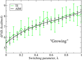
Figure 1: The slope of the free energy d$F$/d$\lambda$ as a function of $\lambda$ for changing the Lennard-Jones size of a neutral particle in a box of explicit water. Results for both TI and AIM methods are shown for $10^{6}$ dynamics steps. The data show the averages (data points) and standard deviations (error bars) from 16 independent simulations for each method. The figure demonstrates that AIM has the ability to sample the $\lambda$-path more efficiently, thus producing a much smoother and more precise profile compared to TI. Thus, AIM is preferred over TI for computing the potential of mean force for this system. In addition, the smoothness of the profile suggests that the switching function $U_{\lambda}$ of Eq. (25) used in this report is adequate.

Table 1 demonstrates that, for long simulation times, all methods produce roughly the same average $\Delta F$ estimate. Also, the table clearly shows that, given $10^{6}$ dynamics steps, AIM provides the most precise free energy estimates.

Method	Within 1.0 kcal/mol	Within 0.5 kcal/mol
AIM	23 000	30 000
TI	89 000	181 000
SEPS	140 000	377 000
BSEPS	279 000	444 000
Jarz	18 000	127 000
BJarz	26 000	96 000
Benn	90 000	180 000
FEPF	104 000	191 000
FEPR	60 000	184 000

Table 2: Number of dynamics steps necessary to be within a specified tolerance of the correct result $\Delta F_{\rm long\;sim}$ = 7.23 kcal/mol, average $\Delta F$ estimate at $10^{6}$ dynamics steps for all methods, for growing a Lennard-Jones particle in explicit solvent. The first column is the method used to obtain the estimate. The second column is the number of dynamics steps needed to estimate $\Delta F$ within 1.0 kcal/mol of $\Delta F_{\rm long\;sim}$ with an uncertainty less than 1.0 kcal/mol. The third column is the number of dynamics steps needed to obtain an estimate within 0.5 kcal/mol with an uncertainty less than 0.5 kcal/mol.

Table 2 shows the approximate number of dynamics steps needed by each method to obtain a free energy estimate within a specific tolerance of $\Delta F_{\rm long\;sim}$ (average of all estimates at $10^{6}$ dynamics steps). Note that the number of dynamics steps needed for the SEPS and BSEPS methods are large due to the fact that whole paths must be discarded for equilibration of the path ensemble. For all methods except AIM, the table entries for Table 2 were estimated using linear interpolation of the data in Table 1. From the data in Table 2, if the desired precision is less than 1.0 kcal/mol, then AIM, Jarz and BJarz appear to be the best methods. However, if the desired precision is less than 0.5 kcal/mol, then AIM is the best choice.

Tables 1 and 2, taken together, demonstrate the difference between using equilibrium data in the “forward” (FEPF) and “reverse” (FEPR) directions. While, the results are similar for $10^{6}$ dynamics steps, it is clear that FEPR produces the desired results more rapidly than FEPF indicating that the configurational overlap is greater in the reverse direction. However, the FEPR data also tends to “overshoot” the correct value by a small margin which makes convergence of the FEPR estimate difficult to judge.

Thus, we conclude that, for growing a Lennard-Jones particle in explicit solvent, the preferred method depends upon the type of estimate one wishes to generate. If a very precise high-quality estimate is desired, then AIM is the best choice by a considerable margin. If a very rapid estimate of $\Delta F$, with an uncertainty of less than 1.0 kcal/mol, is desired, then then comparable results are seen using AIM, Jarz and BJarz methodologies. If the $\Delta F$ estimate is to be within 0.5 kcal/mol, then AIM is the best choice.

Finally, if the desired result is the potential of mean force, then AIM will generate a much smoother curve than TI.

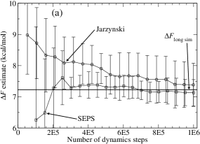
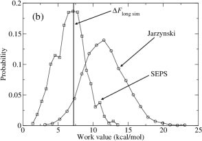
Figure 2: (a) “Fast-growth” uni-directional free energy difference estimates obtained for changing the Lennard-Jones size of a neutral particle in a box of explicit water. Results are shown for both SEPS and Jarz methods as a function of the number of dynamics steps used in the simulation. For both methods, fast-growth work values were generated by simulating roughly 2000 dynamics steps per path, which is ten times shorter than optimal. The solid horizontal line represents the best estimate of the free energy difference $\Delta F_{\rm long\;sim}$ based on averaging all results shown in Table 1 at $10^{6}$ dynamics steps. The averages (data points) and standard deviations (errorbars) are from 16 independent simulations. (b) Histograms of the work values used to generate the free energy estimates for both the SEPS and Jarz methods. The plots demonstrate the potential usefulness of using path sampling over regular Jarzynski averaging. Specifically, if the work values are fast-growth and uni-directional, then SEPS is able to bias the work values in such a way to improve the free energy estimate. Note that for all the SEPS data shown, the first 50 work values are thrown away for equilibration as, described in Sec. IV.5.

V.1.1 Fast-growth uni-directional data

We now consider non-equilibrium uni-directional fast-growth data, i.e., generated by switching the system rapidly from $U_{0}$ (small particle) to $U_{1}$ (large particle). Importantly, there will be an advantage to generating uni-directional data in some cases, since only the $U_{0}$ equilibrium ensemble is needed to estimate $\Delta F$.

In contrast to the data shown in Tables 1 and 2, where the lengths of the non-equilibrium switching trajectories were pre-optimized, here we focus on the efficacy of the methods using non-optimal, rather fast switching. After all, when attempting a free energy computation on a new system, there is no way to know in advance the optimal path length (number of $\lambda$-steps). Substantial optimization may be needed for both SEPS and Jarz methods to work efficiently.

Here, we test the SEPS and Jarz methods using short paths with an equal number of dynamics steps. For SEPS, 500 $\lambda$-steps with four dynamics steps at each value of $\lambda$ was used, producing a distribution of work values with $\sigma_{W}=2.1$ kcal/mol. For Jarz, 2000 $\lambda$-steps with one dynamics step at each value of $\lambda$ was used, producing a distribution of work values with $\sigma_{W}=2.9$ kcal/mol. Note that these paths are roughly ten times shorter than optimal and thus $\sigma_{W}$ is 3-4 times larger than the optimal value of $\sim k_{B}T$.

Figure 2 gives a comparison between SEPS and Jarz methods for the fast-growth uni-directional paths just described. The upper figure (a) shows the average free energy estimates and standard deviations for both the SEPS and Jarz methods. The lower figure (b) gives the histogram of the work values for each method. Both figures also show the “correct” value $\Delta F_{\rm long\;sim}$, generated from a very long simulation. The figures clearly demonstrate that, for fast-growth data, SEPS has the ability to “shift” the work values such that the $\Delta F$ value is near the center of the work value distribution—rather than in the tail of the distribution as with the Jarz method. Thus, the SEPS results converge more rapidly than Jarz to the correct value of $\Delta F$.

We suggest that the the SEPS method may find the greatest use for the ability to bias fast-growth work values to obtain the correct value of $\Delta F$, as shown here.

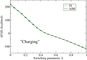
Figure 3: The slope of the free energy d$F$/d$\lambda$ as a function of $\lambda$ for a changing the charge of a Lennard-Jones particle in a box of explicit water from -e/2 to +e/2. Results for both TI and AIM methods are shown for $10^{6}$ dynamics steps. The data show the averages (data points) and standard deviations (error bars) from 16 independent simulations for each method. The errorbars are too small to resolve on the plot shown, however, it should be noted that the average uncertainty in the the slope for AIM is 0.38 kcal/mol and for TI is 1.05 kcal/mol, suggesting that AIM has the ability to produce a more precise profile compared to TI. Thus, AIM is preferred over TI for computing the potential of mean force for this system. The smoothness of the profile also suggests that the switching function $U_{\lambda}$ of Eq. (24) used in this report is adequate.

V.2 Charging a Lennard-Jones particle

We next compute the free energy required to charge a particle from -e/2 to +e/2 in 500 TIP3P waters.

Steps	AIM	TI	SEPS	BSEPS	Jarz	BJarz	Benn	FEPF	FEPR
2E3	8.5(5.5)	24.5(2.3)	—	—	—	—	24.4(2.3)	28.7(2.8)	20.0(2.1)
4E3	9.7(6.6)	21.5(3.0)	—	—	—	—	21.4(3.1)	25.4(3.0)	17.7(3.1)
9E3	14.6(11.4)	20.1(1.7)	—	—	—	—	20.1(1.8)	22.6(1.8)	17.6(2.1)
1.7E4	18.6(10.8)	18.5(1.2)	—	—	—	—	18.5(1.2)	20.3(1.1)	16.8(1.4)
3.5E4	19.7(4.6)	18.44(0.87)	—	—	19.15(0.70)	18.42(0.74)	18.39(0.90)	19.56(1.05)	17.34(0.70)
7E4	18.42(0.43)	18.38(0.69)	—	—	18.82(0.61)	18.29(0.40)	18.33(0.69)	19.18(0.87)	17.64(0.69)
1.3E5	18.41(0.26)	18.34(0.71)	—	—	18.72(0.55)	18.20(0.46)	18.28(0.72)	18.76(0.83)	17.78(0.80)
2.7E5	18.27(0.21)	18.35(0.45)	18.47(1.03)	18.23(0.59)	18.55(0.42)	18.16(0.29)	18.29(0.45)	18.62(0.54)	18.09(0.46)
5.5E5	18.26(0.13)	18.28(0.28)	18.25(0.49)	18.43(0.43)	18.44(0.32)	18.13(0.19)	18.20(0.29)	18.28(0.39)	18.25(0.26)
1E6	18.23(0.13)	18.28(0.30)	18.23(0.30)	18.30(0.42)	18.32(0.26)	18.18(0.16)	18.21(0.31)	18.20(0.33)	18.25(0.31)

Table 3: Free energy difference estimates obtained for changing the charge of a Lennard-Jones particle from -e/2 to +e/2 in a box of explicit water. Results are the averages from 16 independent simulations for various methods described in the text as a function of the number of dynamics steps used in the simulation. The standard deviation is shown in parentheses. For single-ensemble path sampling (SEPS and BSEPS) and Jarzynski methods (Jarz and BJarz), only the most efficient results are shown. The table shows that in the limit of long simulation times ($10^{6}$ dynamics steps) all methods produce average $\Delta F$ estimates that roughly agree. The table also shows that AIM and BJarz approaches provide the most precise long-simulation estimate.

Figure 3 shows the slope of the free energy (${\rm d}F/{\rm d}\lambda=\langle{\rm d}U/{\rm d}\lambda\rangle_{\lambda}$) as a function of $\lambda$ for both TI (green) and AIM (black) after $10^{6}$ Langevin dynamics steps. The data shown in the plot are the mean (data points) and standard deviation (errorbars) for 16 independent trials. While the errorbars are too small to resolve on the plot shown, the average uncertainty in the the slope for AIM is 0.38 kcal/mol and for TI is 1.05 kcal/mol, suggesting that AIM has the ability to produce more precise slope data compared to TI.

Table 3 shows $\Delta F$ estimates for the different approaches. For all non-equilibrium approaches, only the most efficient data are shown. For SEPS and BSEPS the paths were composed of 500 $\lambda$-steps (restricted to 500 due to computer memory) with 80 dynamics steps at each value of $\lambda$. For Jarz the paths were composed of 40 000 $\lambda$-steps with one dynamics step at each value of $\lambda$, and for BJarz, 20 000 $\lambda$-steps with one dynamics step at each value of $\lambda$ were used. For all of these non-equilibrium data, the standard deviation of the work values were $\sigma_{W}\approx 0.8\;{\rm kcal/mol}\approx 1.3\;k_{B}T$, in agreement with previous studies Hummer (2001); Crooks (2000), and with the growing data in this study. At least four different path lengths were attempted for each non-equilibrium method to determine the most efficient.

Table 3 demonstrates that, for long simulation times, all methods produce roughly the same average $\Delta F$ estimate. Also, the table shows that, given $10^{6}$ dynamics steps, AIM and BJarz methodologies provide the most precise free energy estimates.

Tables 3 and 4 show the difference between using equilibrium data in the “forward” (FEPF) and “reverse” (FEPR) directions. While, the results are similar for $10^{6}$ dynamics steps, it is clear that FEPF produces the desired results more rapidly than FEPR indicating that the configurational overlap is greater in the forward direction. However, the FEPF data also tends to “overshoot” the correct value by a small margin which makes convergence of the FEPF estimate difficult to judge.

Method	Within 1.0 kcal/mol	Within 0.5 kcal/mol
AIM	52 000	64 000
TI	27 500	243 000
SEPS	291 000	515 000
BSEPS	399 000	487 000
Jarz	40 000	180 000
BJarz	40 000	69 000
Benn	29 000	245 000
FEPF	43 000	335 000
FEPR	26 000	252 000

Table 4: Number of dynamics steps necessary to be within a specified tolerance of the correct result $\Delta F_{\rm long\;sim}$ = 18.24 kcal/mol, average $\Delta F$ estimate at $10^{6}$ dynamics steps for all methods, for charging a Lennard-Jones particle in explicit solvent. The first column is the method used to obtain the estimate. The second column is the number of dynamics steps needed to estimate $\Delta F$ within 1.0 kcal/mol of $\Delta F_{\rm long\;sim}$ with an uncertainty less than 1.0 kcal/mol. The third column is the number of dynamics steps needed to obtain an estimate within 0.5 kcal/mol with an uncertainty less than 0.5 kcal/mol.

For fast estimation of free energy differences, Table 4 shows the number of dynamics steps needed by each method to obtain a free energy estimate within a specific tolerance of $\Delta F_{\rm long\;sim}$ (average of all estimates at $10^{6}$ dynamics steps). Note that the number of dynamics steps needed for the SEPS and BSEPS methods are large due to the fact that many paths must be discarded for equilibration of the path ensemble. For all methods except AIM, the entries in Table 4 were estimated using linear interpolation of the data in Table 3. From the data in the table, if the desired precision is less than 1.0 kcal/mol, then all methods other than SEPS and BSEPS produce comparable results. However, if the desired precision is less than 0.5 kcal/mol, then AIM and BJarz approaches are best.

We conclude that, when charging a Lennard-Jones particle in explicit solvent, the preferred methodology depends upon the type of estimate one wishes to generate. If a very high quality estimate is desired, then AIM is the best choice, closely followed by BJarz. If a very rapid estimate of $\Delta F$, with an uncertainty of less than 1.0 kcal/mol, is desired, then then comparable results are seen using all methodologies except for SEPS and BSEPS. If the $\Delta F$ estimate is to be within 0.5 kcal/mol, then AIM and BJarz are the best choices.

Finally, if the desired result is the potential of mean force, then AIM will generate a much smoother curve than TI.

V.3 A second look at a two-dimensional model

Because SEPS proved orders of magnitude more efficient than TI and Jarz in the study of a two-dimensional model Ytreberg and Zuckerman (2004a), we return to that model in an effort to understand the decreased effectiveness of SEPS in the present study. Specifically, we use the model from Ref. Ytreberg and Zuckerman, 2004a, but now for a wide range of conformational sampling barrier heights (fixed $\lambda$), and then compare SEPS to TI, as in our original study. Note, that we use the term “conformational sampling barrier” to distinguish it from the barrier in $\lambda$-space.

Some alterations to our approach in Ref. Ytreberg and Zuckerman, 2004a were necessary to provide a fair comparison in the context of the present report. The results in Ref. Ytreberg and Zuckerman, 2004a were obtained for very short paths, large perturbations of the shoot point, and a conformational sampling barrier height of 14.0 $k_{B}T$. For consistency with the present studies, SEPS results were generated with no perturbation of the shoot point, much longer paths, and for a range of conformational sampling barrier heights. Both TI and SEPS simulations utilized Brownian dynamics to propagate the system. For SEPS, paths were generated as described in the present report (but with no velocity), and accepted with the probability given in Eq. (19).

Barrier ($k_{B}T$)	SEPS long	SEPS short	TI
1.0	60 000	200 000	15 300
2.0	120 000	500 000	35 700
4.0	400 000	1 000 000	204 000
6.0	1 400 000	1 400 000	1 020 000
8.0	8 000 000	1 600 000	5 100 000
10.0	40 000 000	2 400 000	20 400 000
12.0	80 000 000	4 000 000	76 500 000
14.0	200 000 000	10 000 000	204 000 000

Table 5: Number of dynamics steps necessary to be within 0.5 $k_{B}T$ of the analytical result for $\Delta F$ with a 0.5 $k_{B}T$ or less standard deviation for the two-dimensional model in Ytreberg and Zuckerman (2004a). The first column is the barrier height of the potential energy surface in $k_{B}T$ units. The second and third columns are the number of dynamics steps using SEPS with, respectively, 200 work values and 20 000 work values. The fourth column is the number of dynamics steps using TI with using 51 equally spaced values of $\lambda$. For both TI and SEPS, half of the generated data were thrown away for equilibration.

Results for the two-dimensional model using SEPS and TI are shown in Table 5. The free energy change is for switching between a single-well potential and a double-well potential with a conformational barrier height in $k_{B}T$ units given in the first column. The next three columns give the number of dynamics steps needed for the $\Delta F$ estimate to be within 0.5 $k_{B}T$ of the correct value with 0.5 $k_{B}T$ or smaller standard deviation (estimated over at least 100 trials): the second and third columns are for SEPS where either 200 (long trajectories) or 20 000 (short trajectories) work values were generated with 50% of the work values discarded for equilibration, and the fourth column is TI using 51 evenly spaced values of $\lambda$ with 50% of the data at each value of $\lambda$ discarded for equilibration.

Table 5 clearly shows that, for very low conformational barrier height, TI is much more efficient than SEPS, and that the most efficient SEPS is obtained using longer paths and thus fewer work values. For increasing conformational barrier heights, SEPS using long paths and TI become comparable, while SEPS using short paths becomes the most efficient. For the largest conformational barrier height tested in this study (14.0 $k_{B}T$), SEPS using short paths is at least 20 times more efficient than either TI or SEPS using long paths.

Since the results for growing and charging an ion in solvent showed that TI was more efficient than SEPS, we suggest that the free energy landscapes for the molecular systems used in this study have rather modest conformational sampling barriers Elber and Czerminski (1990); Zuckerman and Lyman (2006).

VI Conclusions

We have carefully studied several computational free energy difference ($\Delta F$) methods, comparing efficiency and precision. The test cases used for the comparison were relative solvation energy calculations involving either a large change in the Lennard-Jones size or in the charge of a particle in explicit solvent. Specifically, we compared: adaptive integration (AIM) Fasnacht et al. (2004); thermodynamic integration (TI) Kirkwood (1935); path sampling of non-equilibrium work values using both a Jarzynski uni-directional formalism (SEPS) Ytreberg and Zuckerman (2004a), and a Bennett-like bi-directional formalism (BSEPS); Jarzynski (Jarz) Jarzynski (1997a) and Bennett (BJarz) Crooks (2000); Shirts et al. (2003a) averaging of non-equilibrium work values; equilibrium Bennett (Benn) Bennett (1976); and free energy perturbation (forward, FEPF and reverse FEPR) Zwanzig (1954).

AIM Fasnacht et al. (2004) was found to provide very high quality, precise estimates, given long simulation times ($10^{6}$ total dynamics steps in this study), and also allowed very rapid estimation of $\Delta F$. In addition, AIM provided smooth free energy profiles (and thus smooth potential of mean force curves) as compared to TI; see Figs. 1 and 3. Clearly, AIM was the best all-around choice for the systems studied here.

BJarz Crooks (2000) was also found to perform very well, with long-simulation results that were second only to AIM. However, it should be noted that the data shown in this study are for the most efficient path lengths only. To determine the optimal path length, many simulations were performed, adding to the overall cost of the method. Also, our results showed that using bi-directional data (BJarz) produced considerably more precise results than using uni-directional data (Jarz).

The SEPS method is shown to provide accurate free energy estimates from “fast-growth” uni-directional non-equilibrium work values. Specifically, in cases where the standard deviation of the work values is much greater than $k_{B}T$ ($\sigma_{W}\gg k_{B}T$), the SEPS method can effectively shift the work values to allow for more accurate $\Delta F$ estimation than is possible using ordinary Jarzynski averaging. Interestingly, using bi-directional data (BSEPS) did not increase the precision of the $\Delta F$ estimate, and perhaps made it somewhat worse.

We also find, in agreement with previous studies Hummer (2001); Crooks (2000), that the greatest efficiency for the Jarz approach is when $\sigma_{W}\approx 1\;k_{B}T$. For the first time, we also show that SEPS is also most efficient when $\sigma_{W}\approx 1\;k_{B}T$, for the systems studies in this report.

We have also suggested an explanation—with potentially quite interesting consequences—for the decreased effectiveness of SEPS in molecular systems. By re-examining the two-dimensional model used in our first SEPS paper Ytreberg and Zuckerman (2004a), we find that SEPS can indeed be much more more efficient than TI, but only when the conformational sampling barrier is very high ($\gg k_{B}T$). This suggests that the configurational sampling barriers encountered in the molecular systems studied here are fairly modest, counter to our own expectations. A key question is thus raised: How high are conformational sampling barriers encountered in free energy calculations of “practical interest?” See also Refs. Elber and Czerminski, 1990; Zuckerman and Lyman, 2006.

We remind the reader that the results of this study are valid only for the types of $\Delta F$ calculations we considered—namely, growing and charging a Lennard-Jones particle in explicit solvent. When large conformational changes are important, such as for binding affinities, the results could be significantly different—particularly if large conformational sampling barriers are present.

References

- Jorgensen (2004) W. L. Jorgensen, Science 303, 1813 (2004).
- Sotriffer et al. (2003) C. Sotriffer, G. Klebe, M. Stahl, and H.-J. Bohm, Burger’s Medicinal Chemistry and Drug Discovery, vol. 1 (Wiley, New York, 2003), Sixth ed.
- Pitera and van Gunsteren (2001) J. W. Pitera and W. F. van Gunsteren, J. Phys. Chem. B 105, 11264 (2001).
- Grossfield et al. (2003) A. Grossfield, P. Ren, and J. W. Ponder, J. Am. Chem. Soc. 125, 15671 (2003).
- Singh et al. (1994) S. B. Singh, Ajay, D. E. Wemmer, and P. A. Kollman, Proc. Nat. Acad. Sci. (USA) 91, 7673 (1994).
- Oostenbrink et al. (2000) B. C. Oostenbrink, J. W. Pitera, M. M. van Lipzip, J. H. N. Meerman, and W. F. van Gunsteren, J. Med. Chem. 43, 4594 (2000).
- Fujitani et al. (2005) H. Fujitani, Y. Tanida, I. M., G. Jayachandran, C. D. Snow, M. R. Shirts, E. J. Sorin, and V. S. Pande, J. Chem. Phys. 123, 084108 (2005).
- Fasnacht et al. (2004) M. Fasnacht, R. H. Swendsen, and J. M. Rosenberg, Phys. Rev. E 69, 056704 (2004).
- Ytreberg and Zuckerman (2004a) F. M. Ytreberg and D. M. Zuckerman, J. Chem. Phys. 120, 10876 (2004a), J. Chem. Phys. 121, 5022 (2004).
- Zwanzig (1954) R. W. Zwanzig, J. Chem. Phys. 22, 1420 (1954).
- Kirkwood (1935) J. G. Kirkwood, J. Chem. Phys. 3, 300 (1935).
- Straatsma and McCammon (1991) T. P. Straatsma and J. A. McCammon, J. Chem. Phys. 95, 1175 (1991).
- Bennett (1976) C. H. Bennett, J. Comput. Phys. 22, 245 (1976).
- Shirts and Pande (2005) M. R. Shirts and V. S. Pande, J. Chem. Phys. 122, 144107 (2005).
- Kumar et al. (1992) S. Kumar, J. M. Rosenberg, D. Bouzida, R. H. Swendsen, and P. A. Kollman, J. Comput. Chem. 13, 1011 (1992).
- Jarzynski (1997a) C. Jarzynski, Phys. Rev. Lett. 78, 2690 (1997a).
- Crooks (2000) G. E. Crooks, Phys. Rev. E 61, 2361 (2000).
- Ytreberg and Zuckerman (2004b) F. M. Ytreberg and D. M. Zuckerman, J. Comput. Chem. 25, 1749 (2004b).
- Zuckerman and Woolf (2002) D. M. Zuckerman and T. B. Woolf, Phys. Rev. Lett. 89, 180602 (2002).
- Hummer (2001) G. Hummer, J. Chem. Phys. 114, 7330 (2001).
- Jarzynski (1997b) C. Jarzynski, Phys. Rev. E 56, 5018 (1997b).
- Shirts et al. (2003a) M. R. Shirts, E. Bair, G. Hooker, and V. S. Pande, Phys. Rev. Lett. 91, 140601 (2003a).
- Boresch et al. (2003) S. Boresch, F. Tettinger, M. Leitgeb, and M. Karplus, J. Phys. Chem. B 107, 9535 (2003).
- Mordasini and McCammon (2000) T. Z. Mordasini and J. A. McCammon, J. Phys. Chem. B 104, 360 (2000).
- Shirts et al. (2003b) M. R. Shirts, J. W. Pitera, W. C. Swope, and V. S. Pande, J. Chem. Phys. 119, 5740 (2003b).
- Lybrand et al. (1985) T. P. Lybrand, I. Ghosh, and J. A. McCammon, J. Am. Chem. Soc. 107, 7793 (1985).
- Marinari and Parisi (1992) E. Marinari and G. Parisi, Europhys. Lett. 19, 451 (1992).
- Tidor (1993) B. Tidor, J. Phys. Chem. pp. 1069–1073 (1993).
- Kong and Brooks (1996) X. Kong and C. L. Brooks, J. Chem. Phys. 105, 2414 (1996).
- Wang and Landau (2001) F. Wang and D. P. Landau, Phys. Rev. Lett. 86, 2050 (2001).
- Earl and Deem (2005) D. J. Earl and M. W. Deem, J. Phys. Chem. B 109, 6701 (2005).
- Lu et al. (2003) N. Lu, J. K. Singh, and D. A. Kofke, J. Chem. Phys. 118, 2977 (2003).
- Gore et al. (2003) J. Gore, J. Ritort, and C. Bustamante, Proc. Natl. Acad. Sci. (USA) 100, 12564 (2003).
- Sun (2003) S. X. Sun, J. Chem. Phys. 118, 5769 (2003).
- Atilgan and Sun (2004) E. Atilgan and S. X. Sun, J. Chem. Phys. 121, 10392 (2004).
- Athènes (2002) M. Athènes, Phys. Rev. E 66, 046705 (2002).
- Athènes (2004) M. Athènes, Eur. Phys. J. B 38, 651 (2004).
- Adjanor and Athènes (2005) G. Adjanor and M. Athènes, J. Chem. Phys. 123, 234104 (2005).
- Pratt (1986) L. R. Pratt, J. Phys. Chem. 85, 5045 (1986).
- Bolhuis et al. (2002) P. G. Bolhuis, D. Chandler, C. Dellago, and P. L. Geissler, Annu. Rev. Phys. Chem. 53, 291 (2002).
- Hummer (2004) G. Hummer, J. Chem. Phys. 120, 516 (2004).
- Dellago et al. (1999) C. Dellago, P. G. Bolhuis, and D. Chandler, J. Chem. Phys. 110, 6617 (1999).
- Dellago et al. (1998a) C. Dellago, P. G. Bolhuis, F. S. Csajka, and D. Chandler, J. Chem. Phys. 108, 1964 (1998a).
- Dellago et al. (1998b) C. Dellago, P. G. Bolhuis, and D. Chandler, J. Chem. Phys. 108, 9236 (1998b).
- Ponder and Richard (1987) J. W. Ponder and F. M. Richard, J. Comput. Chem. 8, 1016 (1987), http://dasher.wustl.edu/tinker.
- Andersen (1983) H. C. Andersen, J. Comput. Phys. 52, 24 (1983).
- Jorgensen et al. (1996) W. L. Jorgensen, D. S. Maxwell, and J. Tirado-Rives, J. Am. Chem. Soc. 117, 11225 (1996).
- Yang et al. (2004) W. Yang, R. Bitetti-Putzer, and M. Karplus, J. Chem. Phys. 120, 2618 (2004).
- Elber and Czerminski (1990) R. Elber and R. Czerminski, J. Chem. Phys. 92, 5580 (1990).
- Zuckerman and Lyman (2006) D. M. Zuckerman and E. Lyman, J. Chem. Theory and Comput. 2, 1200 (2006).