Growing Scale-free Small-world Networks with Tunable Assortative Coefficient

Abstract

In this paper, we propose a simple rule that generates scale-free small-world networks with tunable assortative coefficient. These networks are constructed by two-stage adding process for each new node. The model can reproduce scale-free degree distributions and small-world effect. The simulation results are consistent with the theoretical predictions approximately. Interestingly, we obtain the nontrivial clustering coefficient $C$ and tunable degree assortativity $r$ by adjusting the parameter: the preferential exponent $\beta$. The model can unify the characterization of both assortative and disassortative networks.

1 Introduction

In the past few years, no issues in the area of network researching attract more scientists than the ones related to the real networks, such as the Internet, the World-Wide Web, the social networks, the scientific collaboration and so on [1, 2, 3, 4, 5, 6]. Recent works on the complex networks have been driven by the empirical properties of real-world networks and the studies on network dynamics [7, 8, 9, 10, 11, 12, 13, 14, 15, 16, 17, 18, 19, 20, 21, 22, 23, 24, 25, 26, 27, 28, 29]. Many empirical evidences indicate that the networks in various fields have some common topology characteristics. They have a small average distance like random graphs, a large clustering coefficient and power-law degree distribution [1, 2], which are called the small-world and scale-free characteristics. The other characteristic is that the social networks are assortative while almost all biological and technological networks are opposite. The networks with high clustering and small average distance are the small-world model of Watts and Strogatz (WS)[1], while the networks with power-law degree distribution are the scale-free network model of Barab$\acute{a}$si and Albert (BA) [2]. The BA model is a pioneering work in the studies on networks, which suggests that the growth and preferential attachment are two main self-organization mechanisms. Although BA model can generate the power-law degree distributions, its assortative coefficient $r$ equals to zero in the limit of large size thus fail to reproduce the disassortative property that extensively exists in the real-world networks. Recently, some models that can generate either assortative or disassortative networks have been reported [30, 31, 32, 33, 34, 35]. Wang et al. presented a mutual attraction model for both assortative and disassortative weighted networks. The model found that the initial attraction $A$ of the newly added nodes may contribute to the difference of the assortative and disassortative networks [34]. Liu et al. [36] proposed a self-learning mutual selection model for weighted networks, which demonstrated that the self-learning probability $p$ may be the reason why the social networks are assortative and the technological networks are disassortative. However, one should not expect the existence of a omnipotent model that can completely illuminate the underlying mechanisms for the emergence of disassortative property in various network systems. In this paper, beside the previous studies, we exhibit an alternative model that can generate scale-free small-world networks with tunable assortative coefficient, which may shed some light in finding the possible explanations to the different evolution mechanisms between assortative and disassortative networks.

Dorogovtsev et. al [37] proposed a simple model of scale-free growing networks . In this model, a new node is added to the network at each time step, which connects to both ends of a randomly chosen link undirected. The model can be equally described by the process that the newly added node connect to node $i$ preferentially, then select a neighbor node of the node $i$ randomly. Holme and Kim [38] proposed a model to generate growing scale-free networks with tunable clustering. The model introduced an additional step to get the trial information and demonstrated that the average number of trial information controls the clustering coefficient of the network. It should be noticed that the newly added node connect to the first node $i$ preferentially, while connect to the neighbor node of the first node $i$ randomly. In this paper, we will propose a growing scale-free network model with tunable assortative coefficient. Inspired by the above two models, the new node is added into the network by two steps. In the first step, the newly added node connects to the existing nodes $i$ preferentially. In the second step, this node selects a neighbor node $s$ of the node $i$ with probability $k_{s}^{\beta}/\sum_{j\in{\Gamma_{i}}}k_{j}^{\beta}$, where $\beta$ is the parameter named preferential exponent and $\Gamma_{i}$ is the neighbor node set of node $i$. This model will be equal to the Holme-Kim model[37] when $\beta=0$, and the MRGN model[35] when $\beta=1$ Specifically, the model can generate a nontrivial clustering property and tunable assortativity coefficient. Therefore, one may find explanations to various real-world networks by our microscopic mechanisms.

2 Construction of the Model

Our model is defined as following.

(1)

Initial condition: The model starts with $m_{0}$ connected nodes.

(2)

Growth: At each time step, one new node $v$ with $m$ edges is added at every time step. Time $t$ is identified as the number of time steps.

(3)

The first step: Each edge of $v$ is then attached to an existing node with the probability proportional to its degree, i.e., the probability for a node $i$ to be attached to $v$ is

$$\Pi_{i}=\frac{k_{i}}{\sum_{j}k_{j}}.$$ (1)

(4)

The second step: If an edge between $v$ and $w$ was added in the first step, then add one more edge from $v$ to a randomly chosen neighbor $s$ of $w$ with probability $P_{t}$ according to the following probability

$$p_{s}=\frac{k_{s}^{\beta}}{\sum_{v\in\Gamma_{i}}{k_{v}^{\beta}}},$$ (2)

If there remains no pair to connect, i.e., if all neighbors of $w$ were always connected to $v$, do the first step instead.

3 Characteristics of the Model

3.1 Degree distribution

The degree distribution is one of the most important statistical characteristics of networks. Since some real-world networks are scale-free, whether the network is of the power-law degree distribution is a criterion to judge the validity of the model. By adopting the mean-field theory, the degree evolution of individual node can be described as

$$\frac{\partial k_{i}}{\partial t}=P(i)+\sum_{j\in\Gamma_{i}}P(i|j)P(j),$$ (3)

where $P(i)$ denotes the probability that the node $i$ with degree $k_{i}$ is selected at the first step, $P(i|j)$ denotes the conditional probability that node $i$ is a neighbor of node $j$ with degree $k_{j}$ which has been selected at the first step.

According to the preferential attachment mechanism of the first step, one has

$$P(i)=\frac{k_{i}}{\sum_{j}k_{j}}.$$ (4)

The conditional probability $P(i|j)$ can be calculated by

$$P(i|j)=\frac{k_{i}}{\sum_{l\in\Gamma_{j}}k_{l}}.$$ (5)

According to the second step, one has that

$$\frac{\partial k_{i}}{\partial t}=\frac{k_{i}}{\sum_{l}k_{l}}+\sum_{j\in\Gamma_{i}}\Big{(}\frac{k_{i}^{\beta}}{\sum_{s\in\Gamma_{j}}k_{s}^{\beta}}\frac{k_{j}}{\sum_{l}k_{l}}\Big{)}.$$ (6)

If $\beta=0$, we get that

$$\frac{\partial k_{i}}{\partial t}=\frac{k_{i}}{\sum_{l}k_{l}}+\sum_{j\in\Gamma_{i}}\Big{(}\frac{1}{k_{j}}\frac{k_{j}}{\sum_{l}k_{l}}\Big{)}=\frac{2k_{i}}{\sum_{l}k_{l}}.$$ (7)

Then we can get that $P(k)\sim k^{-3}$, which has been proved by Holme and Kim [38]. If $\beta=1$, the following formula can be obtained under the assumption that the present network is non-assortative.

$$\frac{\partial k_{i}}{\partial t}=\frac{k_{i}}{\sum_{j}k_{j}}+\sum_{j\in\Gamma_{i}}\frac{k_{i}}{\langle k\rangle k_{l}}\frac{k_{l}}{\sum_{j}k_{j}}=\frac{2k_{i}}{\sum_{j}k_{j}}.$$ (8)

We can obtain that the degree distribution $p(k)\sim k^{-r}$ obeys the power-law and the exponent $\gamma=3$. The numerical results are demonstrated in Fig. 1. From Fig. 1, we can get that the exponents $\gamma$ of the degree distribution are around -3 when $\beta=-2,-1,0,1,2$. When $\beta>0$, the exponent $\gamma$ would increase slightly as the $\beta$ increases.

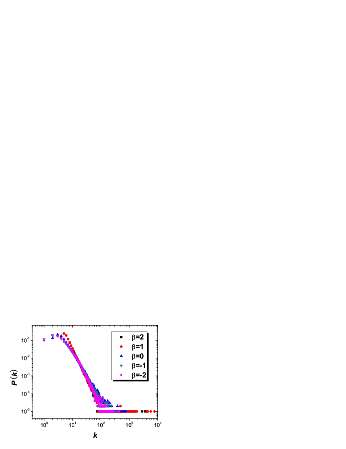
Figure 1: (Color Online) Degree distribution of the present network with $N=100000$ nodes when $m=3$ and $P_{t}=0.3$. In this figure, $p(k)$ denotes the probability of nodes with degree $k$ in the network. The power-law degree distribution exponents $\gamma$ of the four probability density function are $\gamma_{\beta=2}=3.11\pm 0.05$, $\gamma_{\beta=1}=3.11\pm 0.05$, $\gamma_{\beta=0}=2.93\pm 0.04$, $\gamma_{\beta=-1}=2.96\pm 0.05$ and $\gamma_{\beta=-2}=2.95\pm 0.04$.

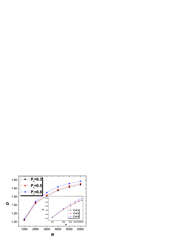
Figure 2: (Color Online) The dependence between the average distance $D$ and the order $N$ of the present network, when $\beta=1$ and $m=4$. One can see that $L$ increases very slowly as ${\rm ln}N$ increases. The inset exhibits the curve where $L$ is considered as a function of $N$. All the data are obtained by 10 independent simulations.

3.2 Average distance

The average distance is also one of the most important parameters to measure the efficiency of communication networks, which is defined as the mean distance over all pairs of nodes. The average distance plays a significant role in measuring the transmission delay. Firstly, we give the following lemma [39].

Lemma 1 For any two nodes $i$ and $j$, each shortest path from $i$ to $j$ does not pass through any nodes $k$ satisfying that $k>{\rm max}\{i,j\}$.

Proof. Denote the shortest path from the node $i$ to $j$ of length $n+1$ by $i\rightarrow x^{1}\rightarrow x^{2}\cdots\rightarrow x^{n}\rightarrow j$($SP_{ij}$), where $n>0$. Suppose that $x^{k}={\rm max}\{x^{1},x^{2},\cdots,x^{n}\}$, if $x^{k}\leq{\rm max}\{i,j\}$, then the conclusion is true. If $x^{k}>{\rm max}\{i,j\}$, denote the youngest node of $SP_{ij}$ by $k$. Denote the subpath passing through node $k$ by $l\rightarrow k\rightarrow r$, where the node $l$ and $r$ are the neighbors of node $k$, then we can prove that node $l$ and $r$ are connected. The shortest path $SP_{ij}$ passes from the node $l$ to $r$ directly, which is conflicted with the hypothesis.

Let $d(i,j)$ represent the distance between node $i$ and $j$ and $\sigma(N)$ as the total distance, i.e., $\sigma(N)=\sum_{1\leq i<j\leq N}d(i,j)$. The average distance of the present model with order $N$, denoted by $L(N)$, is defined as following

$$L(N)=\frac{2\sigma(N)}{N(N-1)}.$$ (9)

According to Lemma 1, the newly added node will not affect the distance between the existing ones. Hence we have

$$\sigma(N+1)=\sigma(N)+\sum^{N}_{i=1}d(i,N+1).$$ (10)

Assume that the $(N+1)$th node is added to the edge $E_{y_{1}y_{2}}$, then Equ. (10) can be rewritten as

$$\sigma(N+1)=\sigma(N)+N+\sum^{N}_{i=1}D(i,y),$$ (11)

where $D(i,y)={\rm min}\{d(i,y_{1}),d(i,y_{2})\}$. Denote $y$ as the edge connected the node $y_{1}$ and $y_{2}$ continuously, then we have the following equation

$$\sigma(N+1)=\sigma(N)+N+\sum_{i=\Lambda}d(i,y),$$ (12)

where the node set $\Lambda=\{1,2,\cdots,N\}-\{y_{1},y_{2}\}$ has $(N-2)$ members. The sum $\sum_{i=\Lambda}d(i,y)$ can be considered as the distance from each node of the network to node $y$ in the present model with order $N-2$. Approximately, the sum $\sum_{i=\Lambda}d(i,y)$ is equal to $L(N-2)$. Hence we have

$$\sum_{i=\Lambda}d(i,y)\approx(N-2)L(N-2).$$ (13)

Because the average distance $L(N)$ increases monotonously with $N$, this yields

$$(N-2)L(N-2)=(N-2)\frac{2\sigma(N-2)}{(N-2)(N-3)}<\frac{2\sigma(N)}{N-1}.$$ (14)

Then we can obtain the inequality

$$\sigma(N+1)<\sigma(N)+N+\frac{2\sigma(N)}{N-1}.$$ (15)

Enlarge $\sigma(N)$, then the upper bound of the increasing tendency of $\sigma(N)$ reads

$$\frac{d\sigma(N)}{dN}=N+\frac{2\sigma(N)}{N-1}.$$ (16)

This leads to the following solution

$$\sigma(N)=(N-1)^{2}{\rm log}(N-1)+C_{1}(N-1)^{2}-(N-1).$$ (17)

The numerical results are demonstrated in Fig. 2.

3.3 Clustering property

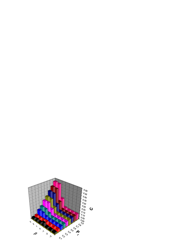
Figure 3: (Color Online) The scale of $C$ with various $\beta$ and $P_{t}$ when $m=3$. The data are averaged over 10 independent runs of network size of $N=6000$.

The small-world characteristic consists of two properties: large clustering coefficient and small average distance. The clustering coefficient, denoted by $C$, is defined as $C=\sum_{i=1}^{N}\frac{C_{i}}{N}$, where $C_{i}$ is the local clustering coefficient for node $i$. $C_{i}$ is

$$C_{i}=\frac{2E(i)}{k_{i}(k_{i}-1)},$$ (18)

where $E(i)$ is the number of edges in the neighbor set of the node $i$, and $k_{i}$ is the degree of node $i$. When the node $i$ is added to the network, it is of degree $m+mP_{t}$ and $E(i)=mP_{t}$. If a new node is added to be a neighbor of $i$ at some time step, $E(i)$ will increase by $mP_{t}$ since the newly added node will connect with one of the neighbors of the node $i$ with probability $P_{t}$. Therefore, in terms of $k_{i}$, the expression of $E(i)$ can be written as

$$E(i)=mP_{t}+P_{t}[k_{i}-(m+mP_{t})].$$ (19)

Hence, we have that

$$C_{i}=\frac{2[mP_{t}+P_{t}(k_{i}-m-mP_{t})]}{k_{i}(k_{i}-1)}=2\Big{(}\frac{mP_{t}^{2}}{k_{i}}+\frac{P_{t}-mP_{t}^{2}}{k_{i}-1}\Big{)}.$$ (20)

This expression indicates that the local clustering scales as $C(k)\sim k^{-1}$, where $C(k)$ denotes the average clustering coefficient value of nodes with degree $k$. It is interesting that a similar scaling has been observed in many artificial models [38, 39, 40, 41] and several real-world networks [42]. The degree-dependent average clustering coefficient $C(k)$ has been demonstrated in Fig. 4. Consequently, we have

$$C=\frac{2}{N}\sum^{N}_{i=1}\Big{(}\frac{mP_{t}^{2}}{k_{i}}+\frac{P_{t}-mP_{t}^{2}}{k_{i}-1}\Big{)}.$$ (21)

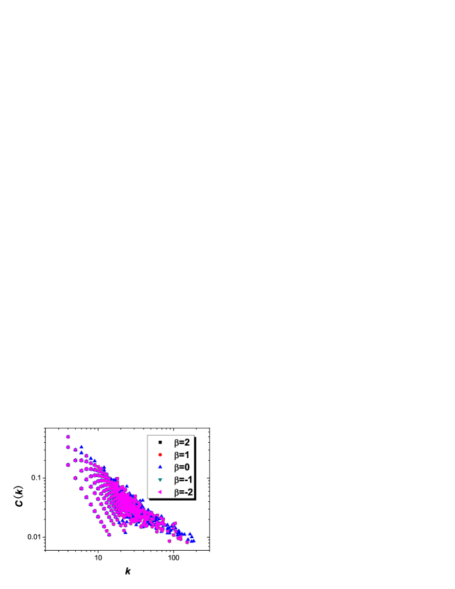
Figure 4: (Color Online) $C(k)$ vs $k$ to various $\beta$ and when $m=3$ and $P_{t}=0.3$. The data are averaged over 10 independent runs of network size of $N=6000$.

Since the degree distribution is $P(k)=ak^{-3}$, where $k=k_{\rm min},\cdots,k_{\rm max}$. The constant $a$ satisfies the normalization equation

$$\sum_{k_{\rm min}}^{k_{\rm max}}ak^{-3}=1,$$ (22)

one can get that $a=2k_{\rm min}^{2}$. The average clustering coefficient $C$ can be rewritten as

$$\begin{array}[]{rcl}C&=&\frac{2}{N}\sum_{k_{\rm min}}^{k_{\rm max}}\Big{(}\frac{NP(k)mP_{t}^{2}}{k}+\frac{NP(k)(P_{t}-mP_{t}^{2})}{k-1}\Big{)}\\[2.0pt] &\approx&2\sum_{k_{\rm min}}^{k_{\rm max}}\Big{(}ak^{-4}mP_{t}^{2}+ak^{-3}(P_{t}-mP_{t}^{2})/(k-1)\Big{)}\\[2.0pt] \end{array}$$ (23)

The numerical results are demonstrated in Fig.3. From figure 3, we can get that if $\beta\leq 0$, the numerical results are consistent with the theoretical predictions approximately, while if $\beta>0$, the fluctuations emerges. The departure from analysis results is observed, which may attribute to the fluctuations of the power-law exponent of degree distribution. It is also helpful to compare the present method with previous analysis approaches on clustering coefficient for Holme-Kim model [43, 44].

3.4 Assortative coefficient

The assortative coefficient $r$ can be calculated from

$$r=\frac{M^{-1}\sum_{i}j_{i}k_{i}-[M^{-1}\sum_{i}\frac{1}{2}(j_{i}+k_{i})]^{2}}{M^{-1}\sum_{i}\frac{1}{2}(j_{i}^{2}+k_{i}^{2})-[M^{-1}\sum_{i}\frac{1}{2}(j_{i}+k_{i})]^{2}},$$ (24)

where $j_{i}$, $k_{i}$ are the degrees of the vertices of the $i$th edge, for $i=1,2,\cdots,M$ [45, 46].

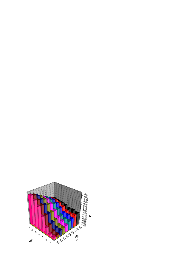
Figure 5: (Color Online) The scale of $r$ with various $\beta$ and $P_{t}$ when $m=1$. The data are averaged over 10 independent runs of network size of $N=6000$.

From Fig. 5, we can find that when $\beta>0$ the assortative coefficient $r$ increases with the probability $P_{t}$, while $r$ decreases with the probability $P_{t}$ when $\beta<0$. As $\beta=0$, $r$ equals to zero approximately.

4 Conclusion and Discussion

In this paper, we propose a simple rule that generates scale-free small-world networks with tunable assortative coefficient. The inspiration of this model is to introduce the parameter $\beta$ to Holme-Kim model. The simulation results are consistent with the theoretical predictions approximately. Interestingly, we obtain the nontrivial clustering coefficient $C$ and tunable degree assortativity $r$, depending on the parameters $\beta$. The model can unify the characterization of both assortative and disassortative networks. Specially, studying the degree-dependent average clustering coefficient $C(k)$ also provides us with a better description of the hierarchies and organizational architecture of weighted networks. Our model may be conducive to future understanding or characterizing real-world networks.

This work has been supported by the Chinese Natural Science Foundation of China under Grant Nos. 70431001, 70271046 and 70471033.

References

- [1] D. J. Watts and S. H. Strogatz, Nature 393 (1998) 440.
- [2] A. -L. Barabsi and R. Albert, Science 286 (1999) 509.
- [3] R. Albert and A. -L. Barabási, Rev. Mod. Phys. 74 (2002) 47.
- [4] S. N. Dorogovtsev and J. F. F. Mendes, Adv. Phys. 51 (2002) 1079.
- [5] M. E. J. Newman, SIAM Rev. 45 (2003) 167.
- [6] X. F. Wang, Int. J. Bifurcat. Chaos 12 (2002) 885.
- [7] W. Li and X. Cai, Phys. Rev. E 69(2004) 046106.
- [8] R. Wang and X. Cai, Chin. Phys. Lett. 22 (2005) 2715.
- [9] P. -P. Zhang, K. Chen, Y. He, T. Zhou, B. -B. Su, Y. -D. Jin, H. Chang, Y. -P. Zhou, L. -C. Sun, B. -H. Wang and D. -R. He, Physica A 360 (2005) 599.
- [10] P. -P. Zhang, Y. He, T. Zhou, B. -B. Su, H. Chang, Y. -P. Zhou, B. -H. Wang and D. -R. He, Acta Physica Sinica 55 (2006) 60.
- [11] M. H. Li, Y. Fan, J. -W. Chen, L. Gao, Z. -R. Di and J. -S. Wu, Physica A 350 (2005) 643.
- [12] J. Q. Fang and Y. Liang, Chin. Phys. Lett. 22 (2005) 2719.
- [13] F. C. Zhao, Y. J. Yang and B. -H. Wang, Phys. Rev. E 72 (2005) 046119.
- [14] H. J. Yang, F. C. Zhao, L. Y Qi and B. L. Hu, Phys. Rev. E 69 (2004) 066104
- [15] J. -G. Liu, Y. -Z. Dang and Z. -T. Wang, arXiv: physics/0509183.
- [16] A. E. Motter and Y. -C. Lai, Phys. Rev. E 66 (2002) 065102.
- [17] K. -I. Goh, D. -S. Lee, B. Kahng and D. Kim, Phys. Rev. Lett. 91 (2003) 148701.
- [18] T. Zhou and B. -H. Wang, Chin. Phys. Lett. 22 (2005) 1072.
- [19] T. Zhou, B. -H. Wang, P. -L. Zhou, C. -X. Yang and J. Liu, Phys. Rev. E 72 (2005) 046139.
- [20] M. Zhao, T. Zhou, B. -H. Wang and W. -X. Wang, Phys. Rev. E 72 (2005) 057102.
- [21] W. Q. Duan, Z. Chen, Z. R. Liu and W. Jin Phys. Rev. E 72 (2005) 026133.
- [22] F. Jin, L. Xiang and F. W. Xiao, Physica A 355 (2005) 657.
- [23] B. Wang, H. W. Tang, C. H. Guo, Z. L. Xiu and T. Zhou, Preprint arXiv:cond-mat/0509711.
- [24] B. Wang, H. W. Tang, C. H. Guo and Z. L. Xiu, Preprint arXiv:cond-mat/0506725.
- [25] J. -G. Liu, Z. -T. Wang and Y. -Z. Dang, Mod. Phys. Lett. B 19 (2005) 785.
- [26] J. -G. Liu, Z. -T. Wang and Y. -Z. Dang, Preprint arXiv:cond-mat/0509290.
- [27] C. P. Zhu, S. J. Xiong, Y. J. Tian, N. Li and K. S. Jiang, Phys. Rev. Lett. 92 (2004) 218702
- [28] F. Comellas, G. Fertin and A. Raspaud, Phys. Rev. E 69 (2004) 037104.
- [29] F. Comellas and M. Sampels, Physica A 309 (2002) 231.
- [30] A. Vázquez, Phys. Rev. E 67, 056104 (2003).
- [31] R. Xulvi-Brunet and I. M. Sokolov, Phys. Rev. E 70 (2004) 066102.
- [32] M. Catanzaro, G. Caldarelli and L. Pietronero, Phys. Rev. E 70 (2004) 037101.
- [33] A. Barrat, M. Barthélemy, R. Pastor-Satorras and A. Vespignani, Proc. Natl. Acad. Sci. U.S.A. 101 (2004) 3747.
- [34] W. -X. Wang, B. Hu, T. Zhou, B. -H. Wang and Y. -B. Xie, Phys. Rev. E 72 (2005) 046140.
- [35] W. -X. Wang, B. -H. Wang, B. Hu, G. Yan and Q. Ou, Phys. Rev. Lett. 94 (2005) 188702 .
- [36] J. -G. Liu, Y. -Z. Dang and Z. -T. Wang, Chin. Phys. Lett. 23(3) (2006) 746.
- [37] S. N. Dorogovtsev, J. F. F. Mendes1 and A. N. Samukhin, Phys. Rev. E 63 (2001) 062101.
- [38] P. Holme and B. J. Kim, Phys. Rev. E 65 (2002) 026107.
- [39] T. Zhou, G. Yan and B. -H. Wang, Phys. Rev. E 71 (2005) 046141.
- [40] J. S. Andrade, H. J. Herrmann, R. F. S. Andrade and L. R. da Silva, Phys. Rev. Lett. 94 (2005) 018702.
- [41] S. N. Dorogovtsev, A. D. Goltsev and J. F. F. Mendes, Phys. Rev. E 65 (2002) 066122.
- [42] E. Ravasz and A. -L. Barabsi, Phys. Rev. E 67 (2003) 026112.
- [43] G. Szabó, M. Alava and J. Kertész, Phys. Rev. E 67 (2003) 056102.
- [44] X. Wu, B. -H. Wang, T. Zhou, W. -X. Wang, M. Zhao and H. -J. Yang, Preprint arXiv: cond-mat/0511655 (Chin. Phys. Lett. In Press).
- [45] M. E. J. Newman, Phys. Rev. Lett. 89 (2002) 208701.
- [46] M. E. J. Newman, Phys. Rev. E 67 (2003) 026126 .