Chromatic dispersion of liquid crystal infiltrated capillary tubes and photonic crystal fibers

Abstract

We consider chromatic dispersion of capillary tubes and photonic crystal fibers infiltrated with liquid crystals. A perturbative scheme for inclusion of material dispersion of both liquid crystal and the surrounding waveguide material is derived. The method is used to calculate the chromatic dispersion at different temperatures.

I Introduction

Together with the development of photonic crystal fibers (PCFs), a large amount of research has been devoted to investigate the possibilities of infiltrating the air holes of a PCF with different liquidskerbage2002optcom , and thereby changing the optical properties of the fiber. Depending on the refractive index of the liquid, the guiding effect of the fiber can possibly be changed from guiding based on modified total internal reflection (mTIR), to guiding based on the photonic band gap effect, where the core has a lower refractive index than the effective index of the cladding. Also selective filling of PCFs, where only some of the holes are infiltrated, has experienced a considerable interestnielsen2005joa ; xiao2005opex ; zografopoulos2006opex , because this can be used to tailor the optical characteristics of the PCF. Among the various liquids that can be infiltrated in a PCF, liquid crystals (LC) distinguishes themselves, because of their anisotropic nature, which allows the possibility of controlling the optical parameters of the waveguide by changing the orientation of the moleculeslarsen2003opex . This orientation can be controlled in different ways, for example by applying an electric field externally. The optical characteristics of the fiber can also be changed by varying the temperature, since the ordinary and extraordinary refractive indices of LCs are highly dependent on temperature. Recently these tunable properties of LCs have been used in various experimental research projectsdu2004apl ; maune2004apl .
The LC can be infiltrated in the PCF using various techniques, one possibility is to use a pressure chamber, but this technique has shown to introduce orientational irregularities in the alignment of LC moleculesphdthesisTanggaard . Another possibility is to infiltrate the holes of the PCF using capillary forces, this technique has shown to give a regular alignment of the LC molecules. A disadvantage using capillary forces for the infiltration is that the length of the infiltrated region will only be of the order of a few centimeters, while longer infiltration lengths can be achieved using pressure infiltration.
In the present work we address the problem of calculating chromatic dispersion curves for different waveguide designs, where the material dispersion of both the LC and waveguide material is taken into account. The LC infiltrated PCF structures we consider have previously been studied theoreticallyzografopoulos2006opex , without inclusion of material dispersion in the PCF material and LC, and only considering the special case where the extraordinary index of the LC and the index of the PCF material were identical. The material dispersion of LC is important to take into account, since LCs are highly dispersive, especially in the visible spectrum, where the dispersion can be much stronger than in for example silica. It has previously been shown that approximating the total dispersion simply by adding the waveguide and material dispersion gives the correct qualitative behavior of the dispersion curveferrando2000ol , but is not sufficient if quantitative data for the dispersion is needed, for example to determine the position of zero dispersion wavelengths (ZDWs).
To calculate precise dispersion profiles, we must therefore include the material dispersion in the field equations. This destroys the well known scalability of Maxwells equations, hence if all the physical dimensions of the fiber are multiplied by a constant factor, we are not able to calculate the new dispersion curve without having to solve the field equations again. In addition, if the computational method used to find the eigenmodes numerically takes the propagation constant as an input variable, and returns the corresponding frequency, we must ensure that this is done in a self-consistent manner, i.e. the values of the dielectric constants in the numerical calculation must correspond to the values of the dielectric constants at the frequency returned by the computational method.
In this work we find the self-consistent frequencies based on a generalization of a perturbative method developed for isotropic waveguideslaegsgaard2003josab . We consider dispersion profiles of both simple waveguides consisting of capillary silica tubes infiltrated with LCs, and more advanced selectively filled PCF structures. Finally we investigate how a change in temperature affects the dispersion characteristics of the fiber.

II Theory

II.1 Alignments of LC-molecules

In all the fiber designs considered in this work the LC is contained inside a hollow circular cylinder. It is well known that an intense optical field will interact with the LC and change the orientation of the moleculestabiryan1986mclc , here we assume that the intensity of the optical field is so weak that we can neglect this interaction. The LC is assumed to be in the nematic phase, where the orientation of the molecules is correlated, resulting in a preferred local orientation of the molecules. This local orientation is described by the director axis $\mathbf{n}(\mathbf{r})$ which is a unit vector pointing in the same direction as the axis of the LC-molecules. In the general case $\mathbf{n}(\mathbf{r})$ is found by minimization of elastic energy. For the cylindrical geometry considered here the director axis has the following form $\mathbf{n}=(\sin(\theta),0,\cos(\theta))$ in cylindrical coordinates $(r,\phi,z)$. $\theta$ is the angle between the director axis $\mathbf{n}$ and the $z$-axis. The alignment of the LC molecules in this situation has previously been studied theoreticallylin1991molcrystliqcryst . $\theta(r)$ can be found by solving a 2nd. order nonlinear ordinary differential equation, where the only parameters are the elastic constants of the LC. We assume that the molecules along $r=0$ are aligned parallel to the $z$-axis ($\theta(0)=0$). The boundary condition at the cylinder wall depends on the LC and the coating of the capillary. Here we consider the two different possibilities $\theta(R)=0$ and $\theta(R)=\pi/2$, where $R$ is the radius of the cylinder. The dielectric tensor of a nematic LC is described in terms of the perpendicular and parallel part of the optical permittivity $\epsilon_{\bot}$ and $\epsilon_{||}$. If the orientation of the molecules is described by the angle $\theta(r)$, then the dielectric tensor has the following form in cylindrical coordinateslin1991molcrystliqcryst

$$\bar{\bar{\epsilon}}=\left(\begin{array}[]{ccc}\epsilon_{rr}&0&\epsilon_{rz}\\ 0&\epsilon_{\phi\phi}&0\\ \epsilon_{zr}&0&\epsilon_{zz}\end{array}\right),$$ (4)

where $\epsilon_{rr}=\epsilon_{\bot}+\Delta\epsilon\sin^{2}\theta$, $\epsilon_{rz}=\epsilon_{zr}=\Delta\epsilon\sin\theta\cos\theta$, $\epsilon_{\phi\phi}=\epsilon_{\bot}$ and $\epsilon_{zz}=\epsilon_{\bot}+\Delta\epsilon\cos^{2}\theta$. $\Delta\epsilon$ is the optical anisotropy defined as $\Delta\epsilon=\epsilon_{||}-\epsilon_{\bot}$. If the 3 elastic constants of the LC describing twist, splay and bend deformations are assumed to be equal, and we further assume that the molecules are aligned parallel with the $z$-axis in the center of the cylinder, the orientation is given by $\theta(r)=2\tan^{-1}(ar/R)$, where $a$ is a constant depending on the boundary condition at the wall. For the boundary conditions considered here we have the two simple analytical solutions $\theta(r)=0$ and $\theta(r)=2\tan^{-1}(r/R)$, depending on whether the molecules are anchored parallel or perpendicular to the boundary of the cylinder. The two orientations are shown schematically in Fig. 1. In the following we will consider these two orientations of the LC molecules, and refer to them as planar ($\theta(r)=0$) and axial ($\theta(r)=2\tan^{-1}(r/R)$) alignment. The planar alignment is easily achieved experimentally, while axial alignment requires that the capillary is coated with a surfactant before the LC is infiltratedphdthesisTanggaard .

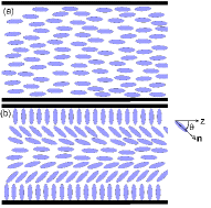
Figure 1: Parallel (a) and axial (b) alignment of LC molecules in a cylindrical geometry. Figures reproduced with permissionphdthesisTanggaard .

II.2 Calculation of chromatic dispersion curves

In this section we derive a perturbative method for calculation of chromatic dispersion of a waveguide infiltrated with LC. The method is general and can be applied to arbitrary waveguide designs. Our method is a generalization of an earlier presented method for isotropic waveguideslaegsgaard2003josab , but this method allows the possibility that the waveguide consists of anisotropic materials. We consider a waveguide which is uniform along the $z$-direction, and therefore assume that the magnetic field can be described in the form of a monochromatic wave travelling along the $z$-direction, i.e. $\mathbf{H}(x,y,z,t)=\exp[i(\beta z-\omega t)]\mathbf{h}(x,y;\beta)$. From Maxwells equations the following equation for the vector field $\mathbf{h}(x,y;\beta)$ is derived

$$\mathbf{\Phi}\mathbf{h} = \frac{\omega^{2}}{c^{2}}\mathbf{h},$$ (5)

$$\mathbf{\Phi} = \nabla_{\beta}\times\bar{\bar{\epsilon}}^{-1}\nabla_{\beta}\times$$ (6)

where the operator $\nabla_{\beta}$ is given by $\nabla_{\beta}=(\partial/\partial x,\partial/\partial y,i\beta)$. $\bar{\bar{\epsilon}}$ is the dielectric tensor, which in the LC region is given by the expression in Eq. (4). In the silica region the dielectric tensor is simply a diagonal matrix, with the dielectric constant of silica in the diagonal. Therefore $\bar{\bar{\epsilon}}=\bar{\bar{\epsilon}}(\mathbf{r},\epsilon_{S}(\omega),\epsilon_{\bot}(\omega),\epsilon_{||}(\omega))$, i.e. the dielectric function depends on position, the dielectric constant of the material surrounding the LC ($\epsilon_{S}$), and the dielectric constants $\epsilon_{\bot}$ and $\epsilon_{||}$ of the LC. Since material dispersion is taken into account, all 3 dielectric constants are assumed to be frequency dependent. The dispersion coefficient is defined by

$$D=\frac{\omega^{2}}{2\pi cv_{g}^{2}}\frac{dv_{g}}{d\omega},$$ (7)

where $v_{g}$ is the group velocity, defined as $v_{g}=\frac{d\omega}{d\beta}$. To find an exact expression for the group velocity we start out by rewriting Eq. (5) as

$$\frac{\langle\mathbf{h},\mathbf{\Phi}\mathbf{h}\rangle}{\langle\mathbf{h},\mathbf{h}\rangle}=\frac{\omega^{2}}{c^{2}}.$$ (8)

Here and in the following we use the following notation for the inner product $\langle\mathbf{A},\mathbf{B}\rangle=\int\mathbf{A}^{*}\cdot\mathbf{B}d\mathbf{r}_{\bot}$, i.e. the integration is over the whole transverse plane. Now the group velocity is found by differentiating both sides of Eq. (8) with respect to the propagation constant $\beta$. The left hand side of Eq. (8) is differentiated with respect to $\beta$ using the Hellman-Feynman theorem. To differentiate the operator $\mathbf{\Phi}$ with respect to $\beta$, we note that the operator depends on $\beta$ explicitly through $\nabla_{\beta}$, and implicitly through the dielectric constants $\epsilon_{j}=\epsilon_{j}(\omega(\beta))$ ($j=S,\bot,||$). In the following $\partial/\partial\beta$ denotes a differentiation for fixed dielectric constants. Using this notation we have the following expression for $\mathbf{\Phi}$ differentiated with respect to $\beta$

$$\frac{d\mathbf{\Phi}}{d\beta}=\frac{\partial\mathbf{\Phi}}{\partial\beta}+v_{g}\sum_{j}\frac{\partial\mathbf{\Phi}}{\partial\epsilon_{j}}\frac{\partial\epsilon_{j}}{\partial\omega}.$$ (9)

Where we have the following expressions for $\partial\mathbf{\Phi}/\partial\beta$ and $\partial\mathbf{\Phi}/\partial\epsilon_{j}$

$$\frac{\partial\mathbf{\Phi}}{\partial\beta} = \nabla_{\beta}\times\bar{\bar{\epsilon}}^{-1}\left(\begin{array}[]{c}0\\ 0\\ i\end{array}\right)\times+\left(\begin{array}[]{c}0\\ 0\\ i\end{array}\right)\times\bar{\bar{\epsilon}}^{-1}\nabla_{\beta}\times$$ (16)

$$\frac{\partial\mathbf{\Phi}}{\partial\epsilon_{j}} = -\nabla_{\beta}\times\bar{\bar{\mathbf{\epsilon}}}^{-1}\frac{\partial\bar{\bar{\mathbf{\epsilon}}}}{\partial\epsilon_{j}}\bar{\bar{\mathbf{\epsilon}}}^{-1}\nabla_{\beta}\times$$ (17)

Using the Hermiticity of the operator $\nabla_{\beta}$, and the Maxwell equation $\nabla_{\beta}\times\mathbf{h}=-i(\omega/c)\bar{\bar{\epsilon}}\mathbf{e}$, now gives us the general expression for the group velocity in the case where the material dispersion $\epsilon_{j}=\epsilon_{j}(\omega)$ is known

$$v_{g} = v_{g}^{0}\left[1+\frac{\omega}{2}\left(\frac{\langle\mathbf{e},\frac{d\epsilon_{S}}{d\omega}\mathbf{e}\rangle_{S}}{\langle\mathbf{h},\mathbf{h}\rangle}\right.\right.$$ (19)

$$+\left.\left.\frac{\langle\mathbf{e},\left(\frac{\partial\bar{\bar{\mathbf{\epsilon}}}}{\partial\epsilon_{\bot}}\frac{d\epsilon_{\bot}}{d\omega}+\frac{\partial\bar{\bar{\mathbf{\epsilon}}}}{\partial\epsilon_{||}}\frac{d\epsilon_{||}}{d\omega}\right)\mathbf{e}\rangle_{LC}}{\langle\mathbf{h},\mathbf{h}\rangle}\right)\right]^{-1},$$

here $\langle\cdot,\cdot\rangle_{S}$ and $\langle\cdot,\cdot\rangle_{LC}$ denote that the integration is only over the silica or the LC respectively. The electric field $\mathbf{e}$ is defined similarly to $\mathbf{h}$, i.e. it is the part of the electric field where the $z$ and $t$ dependence has been factored out. In Eq. (19) $v_{g}^{0}$ denotes the group velocity when the material dispersion is zero. An exact expression for $v_{g}^{0}$ is found by differentiation of Eq. (8) with respect to $\beta$, and again using the Hermiticity of $\nabla_{\beta}$ and the Maxwell equation $\nabla_{\beta}\times\mathbf{h}=-i(\omega/c)\bar{\bar{\epsilon}}\mathbf{e}$ i.e.

$$v_{g}^{0}=\frac{c^{2}}{2\omega}\frac{\langle\mathbf{h},\frac{\partial\mathbf{\Phi}}{\partial\beta}\mathbf{h}\rangle}{\langle\mathbf{h},\mathbf{h}\rangle}=c\frac{Re\langle[\mathbf{e^{*}}\times\mathbf{h}]_{z}\rangle}{\langle\mathbf{h},\mathbf{h}\rangle}.$$ (20)

where $\langle f\rangle=\int fd\mathbf{r}_{\bot}$. Our perturbative method for calculating $D$ consists of several steps, first we make a guess for self-consistent values of the dielectric constants $\epsilon_{i,0}$ and solve Eq. (5). From this solution we find the nonselfconsistent frequency $\omega_{0}$, and the group velocity due to waveguide dispersion $v_{g}^{0}$ by using the definition in Eq. (20). Now generalizing the procedure for isotropic waveguides, we see that a first order approximation to the self-consistent frequency is

$$\omega_{sc}\approx\omega_{0}+\sum_{j}\frac{\partial\omega}{\partial\epsilon_{j}}\Delta\epsilon_{j}=\omega_{0}\left(1-\sum_{j}E_{j}\Delta\epsilon_{j}\right),$$ (21)

where $E_{j}$ ($j=S,\bot,||$) is given by

$$E_{S} = \frac{1}{2}\frac{\langle\mathbf{e},\mathbf{e}\rangle_{S}}{\langle\mathbf{h},\mathbf{h}\rangle},$$ (22)

$$E_{\bot} = \frac{1}{2}\frac{\langle\mathbf{e},\frac{\partial\bar{\bar{\mathbf{\epsilon}}}}{\partial\epsilon_{\bot}}\mathbf{e}\rangle_{LC}}{\langle\mathbf{h},\mathbf{h}\rangle},$$ (23)

$$E_{||} = \frac{1}{2}\frac{\langle\mathbf{e},\frac{\partial\bar{\bar{\mathbf{\epsilon}}}}{\partial\epsilon_{||}}\mathbf{e}\rangle_{LC}}{\langle\mathbf{h},\mathbf{h}\rangle}.$$ (24)

In Eq. (21) $\partial\omega/\partial\epsilon_{j}=-\omega E_{j}$ has been found by differentiating Eq. (8) with respect to $\epsilon_{j}$. $\Delta\epsilon_{j}$ in Eq. (21) is found by noting that

$$\epsilon_{i}(\omega_{sc}) \approx \epsilon_{i}(\omega_{0})+\frac{d\epsilon_{i}}{d\omega}|_{\omega_{0}}(\omega_{sc}-\omega_{0})$$ (25)

$$= \epsilon_{i}(\omega_{0})-\frac{d\epsilon_{i}}{d\omega}|_{\omega_{0}}\sum_{j}E_{j}\Delta\epsilon_{j}\omega_{0}$$ (26)

$$= \epsilon_{i,0}+\Delta\epsilon_{i}.$$ (27)

Eqs. (25) define a system of 3 coupled linear algebraic equations. Once Eqs. (25) have been solved for $\Delta\epsilon_{i}$, our approximation to the selfconsistent frequency is readily found using Eq. (21). Since our goal is to use Eq. (19) for finding the group velocity, we must also find an approximation to $v_{g}^{0}$. This is done by using that

$$\frac{\partial v_{g}^{0}}{\partial\epsilon_{j}}=\frac{\partial^{2}\omega}{\partial\epsilon_{j}\partial\beta}=-\frac{\partial}{\partial\beta}\omega E_{j}=-(v_{g}^{0}E_{j}+\omega\frac{\partial E_{j}}{\partial\beta}).$$ (28)

A first order approximation to the self-consistent group velocity is then found using Eq. (19)

$$v_{g}^{sc}=\frac{v_{g}^{0}-\sum_{j}(v_{g}^{0}E_{j}+\omega_{0}\frac{\partial E_{j}}{\partial\beta})\Delta\epsilon_{j}}{1+\omega_{sc}\sum_{j}E_{j}\frac{d\epsilon_{j}}{d\omega}|_{\omega_{sc}}},$$ (29)

In Eq. (29) and (25) we find the derivatives of the dielectric constants by differentiating the Sellmeier or Cauchy polynomial presented in the following with respect to frequency. $E_{j}$ is found from the fields returned by the computational method, when using the dielectric constants $\epsilon_{i,0}$. Strictly speaking the values of $E_{j}$ used in Eq. (29) should be the values calculated at the selfconsistent frequency. This would require solving Eq. (5) more than one time, and therefore significantly increase the calculation time for each propagation constant, but we have found that the variations in $E_{j}$ with $\epsilon_{i}$ can safely be neglected. The derivatives of $E_{j}$ with respect to $\beta$ are found using a standard three point approximation. After having found the selfconsistent frequencies and the corresponding group velocities for a number of propagation constants $\beta$, we find the dispersion $D$ by using the definition given in Eq. (7), in this calculation the derivative of the group velocity $v_{g}$ with respect to frequency $\omega$ is also approximated using a three point formula.

III Results

Both the planar and axial alignment discussed in the previous section are considered. For the material dispersion of silica we use the Sellmeier curve

$$\epsilon_{SiO_{2}}=1+\sum_{j=1}^{3}\frac{a_{j}\lambda^{2}}{\lambda^{2}-b_{j}},$$ (30)

where $a_{i}$ and $b_{i}$ are constants. Here we use the values in Table 1 as reported by Okamotookamoto .

$i$	$A_{i}^{\bot}(25^{o}$C$)$	$A_{i}^{||}(25^{o}$C$)$	$A_{i}^{\bot}(50^{o}$C$)$	$A_{i}^{||}(50^{o}$C$)$	$a_{i}$	$b_{i}$
$1$	$1.4994$	$1.6933$	1.5062	1.6395	$0.6965325$	$4.368309\cdot 10^{-3}$
$2$	$0.0070$	$0.0078$	0.0063	0.0095	$0.4083099$	$1.394999\cdot 10^{-2}$
$3$	$0.0004$	$0.0028$	0.0006	0.0020	$0.8968766$	$97.93399$

Table 1: Parameters for Cauchy and Sellmeier polynomials given in Eq. (30-31). The non-dimensionless parameters are all given in units of $\mu m^{2}$ or $\mu m^{4}$.

For the LC a Cauchy polynomial is used for both $\epsilon_{\bot}$ and $\epsilon_{||}$

$$\epsilon_{\bot,||}=\left(A_{1}^{\bot,||}+\frac{A_{2}^{\bot,||}}{\lambda^{2}}+\frac{A_{3}^{\bot,||}}{\lambda^{4}}\right)^{2}$$ (31)

where $A_{i}^{\bot,||}$ are constants. Here we use the values for the liquid crystal E7 given in Table 1 as reported by Li et alli2005jap at $25^{o}$C and $50^{o}$C. The values obtained for the dielectric constants using these parameters in the Cauchy polynomials have been shown to be consistent with measured values throughout the visible spectrum and far into the infrared spectrum. In Fig. 2 we have plotted the three dielectric constants $\epsilon_{S}$, $\epsilon_{\bot}$ and $\epsilon_{||}$ as a function of vacuum wavelength.

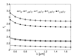
Figure 2: Dielectric constants of silica and E7. The curves for silica and E7 are based on the Sellmeier expression given in Eq. (30) and the Cauchy polynomial given in Eq. (31) respectively. The parameters given in Table 1 are used.

We see that the dielectric constant of silica ($\epsilon_{S}$) is below the two dielectric constants of E7 ($\epsilon_{\bot}$ and $\epsilon_{||}$) throughout the visible spectrum and into the near infrared spectrum, hence a waveguide based on TIR can be realized in this spectrum. In the following we examine the chromatic dispersion for different waveguides based on TIR for the capillary tubes, and modified TIR for the PCFs. Whenever the perturbative method is used to obtain self-consistent frequencies, the guesses for the self-consistent values of the dielectric constants $\epsilon_{j,0}$ are taken to be the values corresponding to a vacuum wavelength of $1\mu$m. We solve Eq. (5) using a freely available software packagejohnson2001:mpb where the electric field is expanded in plane waves. In this software package periodic boundary conditions are assumed on all boundaries, therefore all calculations for both the single capillary and the PCF structure are done using a supercell which is considerably larger than the LC infiltrated cylinder in order to minimize interactions between the images. In this work the distance between repeated images was 14 relative to the radius of the LC infiltrated cylinder for the capillary tubes, and 14 relative to the pitch for the PCF structures. Each elementary cell of the supercell consisted of a uniform $32\times 32$ grid. The relative error using these parameters was estimated to be below $5\%$, by repeating a set of the computations on a finer $64\times 64$ grid.

III.1 Capillary tube infiltrated with LC

First we consider a simple waveguide consisting of a circular hole containing LC surrounded by a silica cladding. Such a waveguide can be realized physically by infiltrating a capillary tube with LC. If we assume that the LC molecules align in the planar orientation discussed in the previous section, the dielectric tensor in Eq. (4) only has nonzero elements in the diagonal, i.e. $\bar{\bar{\epsilon}}=diag(\epsilon_{\bot},\epsilon_{\bot},\epsilon_{||})$. If we further assume the cladding has infinite width, an analytical solution to Eq. (5) can be deriveddai1991josaa . We can therefore use this solution to investigate the accuracy of our numerical perturbative method. The fundamental mode of the waveguide considered here is always the HE₁₁ mode. For a certain mode to be guided in this structure, the propagation constant $\beta$ must satisfy $\epsilon_{S}^{1/2}k<\beta<\epsilon_{\bot}^{1/2}k$, where $k$ is the vacuum wavenumber $k=\omega/c$. The fiber has a single guided mode when the $V$-parameter ($V=kr(\epsilon_{\bot}-\epsilon_{SiO_{2}})^{1/2}$) is less than $2.405$, where $r$ is the inner radius of the tube. In the following we consider fibers with radii of $1.5\mu$m, $1.0\mu$m and $0.75\mu$m, these fibers are single mode for wavelengths larger than $1.63\mu$m, $1.06\mu$m and $0.81\mu$m respectively. In Fig. 3 we have compared the chromatic dispersion found analytically with the chromatic dispersion found using the numerical method described above, together with the perturbative method described in the theory section.

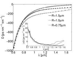
Figure 3: Chromatic dispersion of the fundamental HE₁₁ mode for planar alignment of LC molecules and different radii of the capillary tube. The lines show the chromatic dispersion found using the exact analytical result for the dispersion relation, and markers show the result found numerically together with our perturbative method. The inset shows the absolute difference between the two results, i.e. $|\Delta D|=|D_{exact}-D_{perturbative}|$.

We see that the dispersion curves found numerically together with the perturbative method are quantitatively consistent with the exact dispersion curves. In the inset in Fig. 3 the difference between the analytical result and the perturbative result is also plotted, we see that the smallest deviations between the two results occur in the infrared region, this is also expected since the material dispersion is lowest in this region (see Fig. 2). The relative error of the perturbative method is below $5$% in the wavelength interval from $0.6\mu$m to $1.7\mu$m. The dispersion is very high in the visible spectrum, which is mainly due to the high material dispersion in this region. Also notice that the dispersion is normal ($D<0$) for all the wavelengths and radii considered for the planar alignment.
For the axial alignment of the LC molecules there only exists an analytical solution to Eq. (5) for the TE modeslin1991molcrystliqcryst . But since the fundamental mode, i.e. the mode with the lowest frequency, is not a TE-mode we must solve Eq. (5) numerically to find the chromatic dispersion for the fundamental mode. It turns out that at short wavelengths the fundamental mode is the TM₀₁ mode, while for longer wavelengths the fundamental mode is the hybrid HE₁₁ mode. For the tube radii and wavelengths considered here, the capillary tubes with the axial orientation are always multimoded. Here we consider the two modes with lowest frequency; the HE₁₁ and TM₀₁ mode. The dispersion of these modes as a function of vacuum wavelength is shown in Fig. 4.

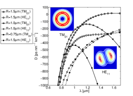
Figure 4: Chromatic dispersion for axial alignment of LC molecules and different radii of the capillary tube. The self-consistent frequencies are found using the perturbative method. Examples of $|\mathbf{H}|^{2}$ for the TM₀₁ and HE₁₁ mode are shown on the insets.

Again we see that the dispersion is mostly normal for the wavelengths and tube radii considered here. But for $r=1.5\mu$m the dispersion becomes anomalous for vacuum wavelengths higher than approximately $1.4\mu$m for the TM₀₁ mode. For $r=1.0\mu$m the fundamental mode switches from the HE₁₁ mode to the TE₀₁ mode at a vacuum wavelength around $\lambda=1\mu$m. For $r=0.75\mu$m and $r=1.5\mu$m the switch between the two modes happens below $\lambda=0.6\mu$m and above $\lambda=1.7\mu$m respectively. In an experimental setup light is coupled into the LC infiltrated region using the HE₁₁ mode of a single mode step index fiber which is an even mode. Therefore it will most likely be easiest to excite the HE₁₁ mode of the LC infiltrated region, since this mode is also even, in contrast to the TM₀₁ which is odd. This is demonstrated in Fig. 5, where the real part of the $x$-component of $\mathbf{H}$ is plotted for the TM₀₁ and HE₁₁.

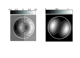
Figure 5: Representative contour plots of real part of the $x$-component of $\mathbf{H}$ for the TM₀₁ mode (left) and the HE₁₁ mode (right) for the axial alignment in a capillary tube. The white circle shows the boundary of the LC infiltrated capillary.

A similar behavior is found for the other components of the $\mathbf{H}$-field, hence the TM₀₁ mode is odd (even though the intensity plot of $|\mathbf{H}|^{2}$ in Fig. 4 is even), and the HE₁₁ mode is even.
In the following the effect of increasing the temperature to $50^{o}$C will be studied. We do not consider temperatures above $50^{o}$C, since the clearing temperature, i.e. the temperature where $\epsilon_{\bot}=\epsilon_{||}$, is around $57^{o}$C for E7li2005jap . Above the clearing temperature the LC is no longer in the anisotropic nematic phase. The parameters for the ordinary and extraordinary indices of refraction at $50^{o}$C can also be found with Cauchy polynomials. The coefficients at $50^{o}$C are given in Table 1, and the dielectric constants at $50^{o}$C are plotted in Fig. 2. We see that the increase in temperature also increases the ordinary dielectric constant, while the extraordinary dielectric constant is lowered. In subplot (a) and (b) in Fig. 6 the effect of raising the temperature to 50^oC is shown for the capillary tube with the planar and axial alignment of the LC molecules.

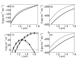
Figure 6: Chromatic dispersion at $25^{o}$C (solid lines) and at $50^{o}$C (dashed lines) for HE₁₁ modes. (a)-(b) Capillary tube ($R=1.0\mu$m) with LC parallel and axially aligned respectively. (c)-(d) Selectively filled PCF structure as shown in inset in Fig. 7 with LC parallel and axially aligned respectively. In subplot (c) the bullets ($\bullet$) and circles ($\circ$) are for $R=0.75\mu$m and $R=1.0\mu$m respectively. The dispersion profile in (d) is for $R=1.0\mu$m.

We see that the dispersion increases for both alignments. For the planar alignment the explanation for this is straight forward. The HE₁₁ mode carries most of its energy in the transverse components of the field, and since the transverse components experiences the ordinary dielectric constant, which increases with temperature, the temperature increase effectively increases the index difference between the core and cladding. The increased index difference gives rise to the higher dispersion. For the axial alignment the explanation for the increased dispersion is more complicated than for the planar alignment. Here a field which is mostly transverse will experience $\epsilon_{\bot}$ near the center of the cylinder, and $\epsilon_{||}$ near the wall of the cylinder. Since $\epsilon_{\bot}$ increases and $\epsilon_{||}$ decreases with temperature, as shown in Fig. 2, it is difficult to say a priori whether the dispersion is increased or decreased.

III.2 PCF infiltrated with LC

In this section we consider a PCF-design similar to the structure recently investigated by Zografopoulos et alzografopoulos2006opex . Where the possibility of changing the fiber characteristics by applying an external electric field was considered. The structure has a cladding consisting of airholes placed in a triangular structure and a core hole infiltrated with LC. A cross section of the considered structure is shown in the inset in Fig. 7.

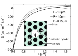
Figure 7: Chromatic dispersion for the PCF structure shown in the inset with different radii of the central hole. The ratios $R/\Lambda=0.6$ and $r/\Lambda=0.3$ are fixed. The LC molecules are planarly aligned. A zoom around the ZDWs is shown in Fig. 6.

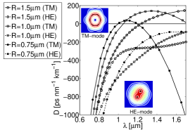
Figure 8: Chromatic dispersion for the PCF structure shown in inset in Fig. 7 with different radii of the central hole. The LC molecules are aligned axially. Examples of $|\mathbf{H}|^{2}$ for the TM and HE mode are shown on the insets.

A physical realization of such a structure will require selective filling, which has recently been demonstratednielsen2005joa ; xiao2005opex , where selective filling was achieved by collapsing the small holes using a fusion splicer, and then the holes with the larger radius were infiltrated. Here we consider a structure where the infiltrated center hole has a radius twice as large as the radius of the cladding holes. The pitch is $5/3$ times the radius of the central hole. Compared to the capillary tube studied in the previous section this structure has a higher index contrast between the core and cladding, because the presence of the airholes significantly lowers the effective index of the cladding. Again we consider both the planar and axial orientation of the LC in the center hole. In Fig. 7 the dispersion curves for different radii of the center hole are shown for the fundamental mode HE-mode with the planar alignment of the LC. The fiber is multimoded for the wavelengths considered here. We see that all the fibers now have regions of both normal and anomalous dispersion. The fiber with a center hole radius of $0.75\mu$m has two ZDWs at $\lambda=1.05\mu$m and $\lambda=1.55\mu$m. The fibers with center hole radii of $1.0\mu$m and $1.5\mu$m each have one ZDW at $\lambda=1.15\mu$m and $\lambda=1.3\mu$m respectively. The dispersion curves for the axial alignment of the LC are shown in Fig. 8. Like the capillary tube with the axial alignment, the type of the fundamental mode is also dependent on the wavelength for the PCF with the LC axially aligned. We see that the fibers with center hole radius $1.0\mu$m and $1.5\mu$m, now have large regions where the dispersion is anomalous for the mode that resembles the TM₀₁ mode of the single capillary tube. For the mode that resembles the HE₁₁-mode of the single capillary tube the dispersion is purely normal for all the waveguide designs considered here.
The effect of increasing the temperature is also investigated for this waveguide design. In plots (c) and (d) in Fig. 6, we see again that the dispersion increases with temperature. In subplot (c) the dispersion profiles for the PCFs with $R=0.75\mu$m and $R=1.0\mu$m are shown. The lower ZDW of the fiber with $R=0.75\mu$m can be tuned between $1.051\mu$m at $25^{o}$C and $1.058\mu$m at $50^{o}$C, while the higher ZDW can be tuned between $1.565\mu$m and $1.571\mu$m. The fiber with $R=1.0\mu$m has one ZDW in the optical spectrum which can be tuned between $1.128\mu$m and $1.139\mu$m. For the PCFs with the axial alignment of the LC molecules we do not have anomalous dispersion for the designs considered here. But the plots for for the axial alignment in Fig. 6 indicates that the dispersion can be tuned in a broader interval for this alignment.

IV Conclusion

An accurate method for calculating chromatic dispersion of anisotropic waveguides is demonstrated. The method is based on a generalization of a previously presented method for isotropic waveguides. We have applied the method to a simple step index fiber with an anisotropic LC core since this problem has an analytical solution. Our results show that the method can be applied to calculate chromatic dispersion curves that are consistent with the exact result throughout the visible spectrum and into the near infrared spectrum.
With the method we have studied chromatic dispersion of capillary tubes and PCFs infiltrated with LC. The considered PCFs are all multimoded in the wavelength intervals considered, while it is shown that single mode operation is possible for the capillary tube infiltrated with LC molecules aligned in parallel. The tunability of the different LC infiltrated waveguides is investigated by calculating the chromatic dispersion at $25^{o}$C and at $50^{o}$C. For the two different alignments of the LC considered here, the tunability is highest for the axial orientation, while the tunability for the planar orientation is weaker. A waveguide design where the ZDWs can be tuned over approximately $10\mu$m is demonstrated.

References

- (1) C. Kerbage, R. Windeler, B. Eggleton, P. Mach, M. Dolinski, and J. Rogers, “Tunable devices based on dynamic positioning of micro-fluids in micro-structured optical fiber,” Opt. Commun. 204, 179–184 (2002).
- (2) K. Nielsen, D. Noordegraaf, T. Sørensen, A. Bjarklev, and T. P. Hansen, “Selective filling of photonic crystal fibers,” J. Opt. A 7, L13–L20 (2005).
- (3) L. Xiao, W. Jin, M. S. Demokan, H. L. Ho, Y. L. Hoo, and C. Zhao, “Fabrication of selective injection microstructured optical fibers with a conventional fusion splicer,” Opt. Express 13, 9014–9022 (2005).
- (4) D. C. Zografopoulos, E. E. Kriezis, and T. D. Tsiboukis, “Photonic crystal-liquid crystal fibers for single-polarization or high-birefringence guidance,” Opt. Express 14, 914–925 (2006).
- (5) T. T. Larsen, A. Bjarklev, D. S. Hermann, and J. Broeng, “Optical devices based on liquid crystal photonic bandgap fibres,” Opt. Express 11, 2589–2596 (2003).
- (6) F. Du, Y.-Q. Lu, and S.-T. Wu, “Electrically tunable liquid-crystal photonic crystal fiber,” Appl. Phys. Lett. 85, 2181–2183 (2004).
- (7) B. Maune, M. Lončar, J. Witzens, M. Hochberg, T. Baehr-Jones, D. Psaltis, A. Scherer, and Y. Qiu, “Liquid-crystal electric tuning of a photonic crystal laser,” Appl. Phys. Lett. 85, 360–362 (2004).
- (8) T. T. Alkeskjold, “Optical devices based on liquid crystal photonic bandgap fibers,” Ph.D. thesis, Department of Communication, Optics & Materials, Technical University of Denmark (2005).
- (9) A. Ferrando, E. Silvestre, J. J. Miret, and P. Andrés, “Nearly zero ultraflattened dispersion in photonic crystal fibers,” Opt. Lett. 25, 790–792 (2000).
- (10) J. Lægsgaard, A. Bjarklev, and S. E. B. Libori, “Chromatic dispersion in photonic crystal fibers: fast and accurate scheme for calculation,” J. Opt. Soc. Am. B 20, 443–448 (2003).
- (11) N. V. Tabiryan, A. V. Sukhov, and B. Y. Zel’dovich, “Orientational optical nonlinearity of liquid crystals,” Mol. Cryst. Liq. Cryst. 136, 1–139 (1986).
- (12) H. Lin, P. Palffy-Muhoray, and M. A. Lee, “Liquid crystalline cores for optical fibers,” Mol. Cryst. Liq. Cryst. 204, 1511–1522 (1991).
- (13) K. Okamoto, Fundamentals of optical waveguides (Academic Press, San Diego, 2000).
- (14) J. Li, S. T. Wu, S. Brugioni, R. Meucci, and S. Faetti, “Infrared refractive indices of liquid crystals,” J. Appl. Phys. 97, 73,501–1–5.
- (15) S. G. Johnson and J. D. Joannopoulos, “Block-iterative frequency-domain methods for Maxwell’s equations in a planewave basis,” Opt. Express 8, 173–190 (2001).
- (16) J. D. Dai and C. K. Jen, “Analysis of cladded uniaxial single-crystal fibers,” J. Opt. Soc. Am. A 8, 2021–2025 (1991).