Theoretical prediction of spectral and optical properties of bacteriochlorophylls in thermally disordered LH2 antenna complexes

Abstract

A general approach for calculating spectral and optical properties of pigment-protein complexes of known atomic structure is presented. The method, that combines molecular dynamics simulations, quantum chemistry calculations and statistical mechanical modeling, is demonstrated by calculating the absorption and circular dichroism spectra of the B800-B850 bacteriochlorophylls of the LH2 antenna complex from Rs. molischianum at room temperature. The calculated spectra are found to be in good agreement with the available experimental results. The calculations reveal that the broadening of the B800 band is mainly caused by the interactions with the polar protein environment, while the broadening of the B850 band is due to the excitonic interactions. Since it contains no fitting parameters, in principle, the proposed method can be used to predict optical spectra of arbitrary pigment-protein complexes of known structure.

I Introduction

Pigment-protein complexes (PPCs) play an important role in photosynthetically active biological systems and have been the subject of numerous experimental and theoretical studies Renger et al., 2001. In a PPC the photoactive pigment molecules are held in well defined spatial configuration and orientation by a scaffold of proteins. The availability of high resolution crystal structure for a continuously growing number of PPCs provides a unique opportunity in better understanding their properties and function at atomic level. The spectral and optical properties of PPCs are determined by (i) the chemical nature of the pigment, (ii) the electronic interactions between the pigment molecules, and (iii) the interactions between pigment molecules and their environment (e.g., protein, lipid, solvent). Since in biological systems PPCs exist and function at physiological temperature their electronic and optical properties are strongly affected by thermal fluctuations which represent the main source of dynamic disorder in these systems.

Unfortunately, even in the simplest theoretical models of PPCs the simultaneous treatment of the electronic coupling between the pigments and the effect of thermal disorder can be done only approximately Chernyak et al. (1998); Mukamel (1995); May and Kühn (2000a); van Amerongen et al. (2000). The purpose of this paper is to formulate and implement an efficient method for calculating spectral and optical properties, e.g., linear absorption (OD) and circular dichroism (CD) spectra of PPCs at finite temperature by using only atomic structure information. To demonstrate its usefulness, we apply the proposed method to calculate the OD and CD spectra at room temperature of the aggregate of bacteriochlorophyll-a (BChl-a) molecules in the LH2 antenna complex from the purple bacterium Rs. molischianum. Following their crystal structure determination, LH2 complexes from Rs. molischianum Koepke et al. (1996) and Rsp. acidophila McDermott et al. (1995) have been extensively studied both experimentally Hu et al. (2002); Yang et al. (2001); Sundstrom et al. (1999); Wu et al. (1997); Beekman et al. (1997); Georgakopoulou et al. (2002); Somsen et al. (1996); Scholes and Fleming (2000) and theoretically Hu et al. (2002); Yang et al. (2001); Sundstrom et al. (1999); Damjanovic et al. (2002a); He et al. (2002); Hu et al. (1998a); Ihalainen et al. (2001); Linnanto et al. (1999); Meier et al. (1997); Ray and Makri (1999); Jang and Silbey (2003). In Rs. molischianum the LH2 is an octamer of $\alpha\beta$-heterodimers arranged in a ring-like structure Hu and Schulten (1997); Hu et al. (1998b). Each protomer consists of an $\alpha$- and a $\beta$-apoprotein which binds non-covalently one BChl-a molecule that absorbs at $800$ nm (referred to as B800), two BChl-a molecules that absorb at $850$ nm (referred to as B850) and at least one carotenoid that absorbs around $500$ nm. The total of 16 B850 and 8 B800 BChls form two circular aggregates, both oriented parallel to the surface of the membrane. The excitonic coupling between the B800s is negligible because of their large spatial separation ($\sim{22}$ Å). Therefore, the optically active Q_y excited electronic states of the B800s are almost degenerate. On the other hand, the tightly packed B850s (with and average Mg$-$Mg distance of $\sim 9.2$ Å within the $\alpha\beta-$heterodimer and $\sim 8.9$ Å between the neighboring protomers) are strongly coupled and the corresponding $Q_{y}$ excited states form an excitonic band in which the states that carry most of the oscillator strength are clustered about $\sim{850}$ nm ($1.46$ eV). Another important difference between the two BChl rings is that while the B800s are surrounded by mostly hydrophilic protein residues the binding pocket of the B850s is predominantly hydrophobic. Koepke et al. (1996) Thus, although both B800s and B850s are chemically identical BChl-a molecules their specific spatial arrangement and the nature of their immediate protein surrounding alter differently their spectral and optical properties. For example, it is quite surprising that the two peaks, due to the B800 and B850 BChls, in the experimental OD spectrum of LH2 from Rs. molischianum at room temperature Zhang et al. (2000); Ihalainen et al. (2001) have comparable widths although, as mentioned above, the B800 levels are almost degenerate while the B850 levels form a $\sim{0.2}$ eV wide excitonic band.

Clearly, novel methods for calculating optical spectra of PPCs by using computer simulations based entirely on the atomic structure of the system would not only provide a better understanding and interpretation of the existing experimental results but would also help in predicting and designing new experiments. The standard procedure to simulate the experimental spectra of LH2 systems (and PPCs in general) consists of two stepsMukamel (1995); Amerongen et al. (2000); May and Kühn (2000a). First, the excitation energy spectrum is determined based on the static crystal structure of the system and, second, the corresponding stick spectrum is “dressed up” with simulated Gaussian (in case of static disorder) and/or Lorentzian (in case of dynamic disorder) line widths characterized by empirically (and often self consistently) determined parameters. Alternatively, the spectral broadening of the stick spectrum can also be described through the coupling of the electronic excitations (modeled as two- or multilevel-systems) to a stochastic heat bath characterized by a model spectral density with empirical parameters. While either approach may yield excellent agreement between the simulated and experimental spectra, the empirical nature of the model parameters restricts their predictive power.

Our proposed method for calculating optical spectra is based on a combination of all atom molecular dynamics (MD) simulations, quantum chemistry (QC) calculations, and quantum many-body theory. The conformational dynamics of the LH2 ring embedded into its natural environment (a fully solvated lipid bilayer) are followed by means of classical MD simulations. Next, for each BChl, modeled as a quantum two level system, the Q_y excitation energy gap and transition dipole moment time series are determined along a properly chosen segment of the MD trajectory by means of QC calculations. Finally, the OD and CD spectra are determined as weighted sums of the Fourier transform of the quantum dipole-dipole correlation function (i.e., the absorption lineshape function) which, within the cumulant approximation, can be calculated from the sole knowledge of the energy gap time series. Formally, this method can also be regarded as a two step procedure. First, a stick spectrum is generated from the average values of the energy gap time series and, second, spectral broadening is applied through the corresponding lineshape function weighted by the mean transition dipole (rotational) strength in the case of OD (CD) spectrum. Since both the peak position and the broadening of the optical spectrum are obtained from the same energy gap time series determined from combined MD/QC calculations, the proposed method requires no empirical fitting parameters making it ideal for predicting optical spectra for PPCs with known structure. Similar MD/QC methods were used previously by Mercer et al. (1999) for calculating the OD spectrum of BChl-a in methanol, and by Damjanovic et al. (2002a) to determine the OD and CD spectra of B850s in LH2 from Rs. molischianum. The relationship between these studies and the present one will be established below.

The reminder of the paper is organized as follows. The theoretical background of the proposed method for calculating optical spectra of PPCs is presented in Sec. II. The employed MC simulations and QC calculations are described in Sec. III. The obtained results and their discussion is contained in Sec. IV. Finally, Sec. V is reserved for conclusions.

II Theory

In order to calculate the linear optical absorption of a PPC we assume that the electronic properties of individual pigment molecules can be described in terms of a two-level system, formed by the ground state and the lowest excited singlet state (e.g., the Q_y state in the case of BChl-a) involved in the optical absorption process. Neglecting for the moment the direct interaction between the pigments (e.g., by assuming a sufficiently large spatial separation between them as in the case of the B800s in LH2), we denote these two states for the $n^{th}$ pigment ($n=1,\ldots N$) as $|0\rangle\equiv|0_{n}\rangle$ and $|n\rangle\equiv|1_{n}\rangle$, respectively. Once the interaction between the pigment and its environment (composed of protein matrix, lipid membrane and solvent molecules) is taken into account these two levels turn into, still well separated, energy bands $|0;\lambda_{0}\rangle=|0\rangle|\lambda_{0}\rangle$ and $|n;\lambda_{n}\rangle=|n\rangle|\lambda_{n}\rangle$, where the quantum numbers $\lambda_{0}$ and $\lambda_{n}$ specify the state of the $n^{th}$ pigment on the ground- and excited-state potential energy surface, respectively. Because the exact quantum mechanical treatment of the eigenstates $|0;\lambda_{0}\rangle$, $|n;\lambda_{n}\rangle$ and of the corresponding energy eigenvalues $\mathcal{E}_{0,\lambda_{0}}$, $\mathcal{E}_{n,\lambda_{n}}$ is not feasible, usually the quantum numbers $\lambda_{0}$ and $\lambda_{n}$ are associated with the vibronic states of the PPC that can be treated within the harmonic approximation. Here we follow a different approach in which the dynamics of the nuclear degrees of freedom of the PPC are described by all-atom MD simulations, and the energy gap time series $\Delta{E}_{n}(t)=\mathcal{E}_{n}(t)-\mathcal{E}_{0}(t)$ is calculated at each MD time step by QC calculations as described below. The main assumption of this approach is that the obtained energy gap time series $\Delta{E}_{n}(t)$ can be used to calculate approximately equilibrium quantities (such as energy gap density of states and time autocorrelation functions) of the original system without the knowledge of the exact energy gap spectrum $\Delta\mathcal{E}_{n,\lambda_{n},\lambda_{0}}=\mathcal{E}_{n,\lambda_{n}}-\mathcal{E}_{0,\lambda_{0}}$.

In the absence of the excitonic coupling between the pigment molecules, the Hamiltonian of the system can be written as $\mathcal{H}=H_{0}+H$, where

$$H_{0}=\sum_{\lambda_{0}}|0;\lambda_{0}\rangle\mathcal{E}_{0,\lambda_{0}}\langle 0;\lambda_{0}|,$$ (1a)

and

$$H=\sum_{n}H_{n}=\sum_{\lambda_{n}}|n;\lambda_{n}\rangle\mathcal{E}_{n,\lambda_{n}}\langle n;\lambda_{n}|\;.$$ (1b)

The dipole moment operator through which the incident light field couples to the $n^{th}$ pigment is given by

$$\hat{\bm{\mu}}_{n}=\sum_{\lambda_{n},\lambda_{0}}\mathbf{d}_{n,\lambda_{n},\lambda_{0}}|n;\lambda_{n}\rangle\langle 0;\lambda_{0}|,$$ (2a)

where the transition dipole moment (TDM) matrix element $$\mathbf{d}_{n,\lambda_{n},\lambda_{0}}$$ in the Condon approximation May and Kühn (2000a) can be written

$$\mathbf{d}_{n,\lambda_{n},\lambda_{0}}\approx\mathbf{d}_{n}\langle\lambda_{n}|\lambda_{0}\rangle.$$ (2b)

Here $\mathbf{d}_{n}=\langle 1|\hat{\bm{\mu}}_{n}|0\rangle$ is the real TDM vector whose time series can be determined from the same combined MD/QC calculations as $\Delta{E}_{n}(t)$. Note that while $\langle 1|0\rangle=0$, in general the Franck-Condon factors $\langle\lambda_{n}|\lambda_{0}\rangle$ are finite May and Kühn (2000a).

When the size of the PPC is much smaller than the wavelength of the light field, in leading approximation the latter can be regarded as homogeneous throughout the system and, according to standard linear response theory, the corresponding OD spectrum is proportional to the dipole-dipole correlation function

$$I(\omega)\propto\omega\sum_{n,m}\text{Re}\left[\int_{0}^{\infty}dte^{i\omega t}\left\langle\hat{\mu}^{\dagger}_{m,i}(0)\hat{\mu}_{n,i}(t)\right\rangle\right],$$ (3)

where $\hat{\mu}_{n,i}(t)=e^{-iHt}\hat{\mu}_{n,i}(0)e^{iH_{0}t}$ is the $i\in\{x,y,z\}$ component of the time dependent electric dipole operator, and $\langle\ldots\rangle=\text{Tr}\left\{Z_{0}^{-1}\exp(-\beta H_{0})\ldots\right\}$ with $\beta=1/k_{B}T$ the usual temperature factor and $Z_{0}$ the corresponding partition function. To simplify notation, throughout this paper we use units in which $\hbar=1$, and apply the convention of implicit summation over repeated vector indices. By employing Eqs. (1)-(2), after some algebra, the quantum dipole correlation function in Eq. (3) can be expressed as

$$\left\langle\hat{\mu}^{\dagger}_{m,j}(0)\hat{\mu}_{n,i}(t)\right\rangle=d_{n,i}d_{m,j}\delta_{nm}\left\langle e^{iH_{0}t}e^{-iH_{n}t}\right\rangle,$$ (4)

where $\delta_{nm}$ is the Kronecker delta. By inserting Eq. (4) into Eq. (3) one obtains the sought OD spectrum of an aggregate of noninteracting pigments in their native environment

$$I(\omega)\propto\omega\sum_{n}d_{n}^{2}A_{n}(\omega),$$ (5a)

where the lineshape function is defined as

$$A_{n}(\omega)=\text{Re}\int_{0}^{\infty}dte^{i\omega t}\left\langle e^{iH_{0}t}e^{-iH_{n}t}\right\rangle.$$ (5b)

The main difficulty in calculating the quantum time correlation function in Eq. (5b) is due to the fact that the Hamiltonians $H_{0}$ and $H_{n}$ do not commute. If they would, then the lineshape function could be expressed in terms of the energy gap density of states (DOS). Indeed, in this case $\left\langle e^{iH_{0}t}e^{-iH_{n}t}\right\rangle\approx\left\langle\exp(-i\Delta{H}_{n}t)\right\rangle$, with $\Delta{H}_{n}=H_{n}-H_{0}$, and by calculating the time integral in Eq. (5b) would follow

$$A_{n}(\omega) \approx\pi\mathcal{N}(\omega)\;,$$ (6a)

$$\mathcal{N}(\omega) \equiv\langle\delta(\omega-\Delta{H}_{n})\rangle\approx\langle\delta(\omega-\Delta{E}_{n}(t))\rangle,$$ (6b)

where the density of states $\mathcal{N}(\omega)$ is approximated by the binned histogram of the energy gap fluctuations $\Delta{E}_{n}(t)$ obtained from combined MD/QC calculations. In general, Eqs. (6) overestimate the broadening of the lineshape function. Indeed, the Fourier transform of the exact spectral representation of the correlation function

$$\left\langle e^{-iH_{0}t}e^{iHt}\right\rangle=\sum_{\lambda_{0},\lambda_{n}}\rho_{\lambda_{0}}|\langle\lambda_{0}|\lambda_{n}\rangle|^{2}e^{-i(\mathcal{E}_{n,\lambda_{n}}-\mathcal{E}_{0,\lambda_{0}})t}\;,$$ (7a)

where $$\rho_{\lambda_{0}}=Z_{0}^{-1}exp(-\beta\mathcal{E}_{0,\lambda_{0}})$$ is the statistical matrix of the electronic ground state, yields

$$A(\omega)=2\pi\sum_{\lambda_{0},\lambda_{n}}\rho_{\lambda_{0}}|\langle\lambda_{0}|\lambda_{n}\rangle|^{2}\delta(\omega-\Delta\mathcal{E}_{n,\lambda_{n},\lambda_{0}})\;,$$ (7b)

which can be regarded as a Franck-Condon weighted and thermally averaged density of stateMay and Kühn (2000b). By setting the Franck-Condon factors $\langle\lambda_{0}|\lambda_{n}\rangle$ equal to unity in (7b) one obtains Eqs. (6). Since it is not possible to determine all these factors, it is often convenient to use Eqs. (6) as a rough estimate of $A_{n}(\omega)$ for calculating the OD spectrum.

A systematic way of calculating the correlation function in (5b) is the cumulant expansion method. Here we employ the second order cumulant approximation that is often used in optical spectra calculationsMukamel (1995). We have

$$\begin{split}\left\langle e^{iH_{0}t}e^{-iH_{n}t}\right\rangle=\left\langle\text{T}\;\exp\left[-i\int_{0}^{t}d\tau\Delta{H}_{n}(\tau)\right]\right\rangle\\ \approx\exp\left[-i\langle\Delta{H}_{n}\rangle t-\int_{0}^{t}d\tau(t-\tau){\cal C}_{n}(\tau)\right],\end{split}$$ (8)

where T is the time ordering operator, $\Delta{H}_{n}(t)=e^{iH_{0}t}\Delta{H}_{n}e^{-iH_{0}t}$, ${\cal C}_{n}(t)=\left\langle\delta{H}_{n}(t)\delta{H}_{n}(0)\right\rangle$, and $\delta{H}_{n}(t)=\Delta{H}_{n}(t)-\left\langle\Delta{H}_{n}\right\rangle$. To make progress, the quantum statistical averages in Eq. (8) will be approximated with classical ones involving the energy gap time series $\Delta{E}_{n}(t)$, i.e.,

$$\left\langle\Delta{H}_{n}\right\rangle\approx\left\langle\Delta{E}_{n}(t)\right\rangle\equiv\omega_{n},$$ (9a)

$$\text{Re}[{\cal C}_{n}(t)]\approx C_{n}(t)\equiv\langle\delta{E}_{n}(t)\delta{E}_{n}(0)\rangle\;,$$ (9b)

where $\delta{E}_{n}(t)=\Delta{E}_{n}(t)-\langle\Delta{E}_{n}\rangle$. While approximating a quantum time correlation function by identifying its real part with the corresponding classical correlation function as in Eq. (9b) is widely used Mercer et al. (1999); Makri (1999); Schulten and Tesch (1991), other approximation schemes have also been considered in the literature Egorov et al. (1999). Next, by invoking the fluctuation dissipation theorem $\widetilde{\cal C}_{n}(-\omega)=\exp(-\beta\omega)\widetilde{\cal C}_{n}(\omega)$, where $\widetilde{\cal C}_{n}(\omega)=\int_{-\infty}^{\infty}dt\,{\cal C}_{n}(t)\exp({i\omega t})$ is the Fourier transform of ${\cal C}_{n}(t)$, the quantum correlation function in terms of the real spectral density

$$J_{n}(\omega)=\frac{1}{2}\left[\widetilde{\cal C}_{n}(\omega)-\widetilde{\cal C}_{n}(-\omega)\right]=\frac{1}{2}\left(1-e^{-\beta\omega}\right)\widetilde{\cal C}_{n}(\omega)$$ (10)

can be written as

$${\cal C}_{n}(t) ={\cal C}^{\prime}_{n}(t)-i{\cal C}^{\prime\prime}_{n}(t)$$ (11)

$$=\int_{0}^{\infty}\frac{d\omega}{\pi}J_{n}(\omega)\left[\coth(\beta\omega/2)\cos\omega t-i\sin\omega t\right]\;.$$

By identifying the real part of Eq. (11) with Eq. (9b) one can determine both the spectral density and the imaginary part of the quantum correlation function, i.e.,

$$J_{n}(\omega)=2\tanh(\beta\omega/2)\int_{0}^{\infty}dt\,C_{n}(t)\cos\omega t,$$ (12)

and

$${\cal C}^{\prime\prime}_{n}(t)=\int_{0}^{\infty}\frac{d\omega}{\pi}J_{n}(\omega)\sin\omega t.$$ (13)

Thus, the lineshape function within the second cumulant approximation is

$$A_{n}(\omega)\equiv\overline{A}_{n}(\omega-\omega_{n})=\int_{0}^{\infty}dt\,e^{-\phi_{n}(t)}\cos[(\omega-\omega_{n})t+\varphi_{n}(t)],$$ (14a)

where the broadening and frequency shift functions are given by

$$\phi_{n}(t)=\int_{0}^{\infty}d\tau\,(t-\tau)C_{n}(\tau)\;,$$ (14b)

and

$$\varphi_{n}(t)=\int_{0}^{\infty}d\omega\,J_{n}(\omega)\frac{\omega t-\sin\omega t}{\omega^{2}}\;.$$ (14c)

A straightforward extension of the above method for calculating the lineshape function and the OD spectrum of $N$ excitonically coupled pigment molecules would require the determination of the energies $\mathcal{E}_{J,\lambda_{J}}$ and TDMs $\mathbf{d}_{J}$ corresponding to the excitonic states $|J;\lambda_{J}\rangle$, $J=1,\ldots,N$. Unfortunately, the required QC calculations (by considering all $N$ pigments as a single quantum system) are still prohibitively expensive computationally. Therefore, we employed an effective Hamiltonian approximation for determining the time series $\Delta{E}_{J}(t)=\mathcal{E}_{J}(t)-\mathcal{E}_{0}(t)$ and $\mathbf{d}_{J}(t)$ from $\Delta{E}_{n}(t)$ and $\mathbf{d}_{n}(t)$ of the individual pigments. Assuming that these are coupled through the usual point dipole-dipole interaction

$$V_{nm}=\frac{1}{4\pi\varepsilon_{0}\varepsilon_{r}}\left[\frac{\mathbf{d}_{n}\mathbf{d}_{m}}{r_{nm}^{3}}-3\frac{(\mathbf{d}_{n}\cdot\mathbf{r}_{nm})\,(\mathbf{d}_{m}\cdot\mathbf{r}_{nm})}{r_{nm}^{5}}\right]\;,$$ (15)

where $\varepsilon_{r}$ is the relative dielectric permitivity of the medium, $\mathbf{r}_{n}$ is the position vector of pigment $n$, and $\mathbf{r}_{nm}=\mathbf{r}_{m}-\mathbf{r}_{n}$, the eigenvalue equation one needs to solve at every MD timestep is

$$\sum_{m}[(\Delta{E}_{n}\delta_{nm}+V_{nm})-\Delta{E}_{J}\delta_{nm}]c_{m}^{(J)}=0\;.$$ (16)

In term of the coefficients $c_{n}^{(J)}=\langle J|n\rangle$ the excitonic TDMs are

$$\mathbf{d}_{J}=\sum_{n}\langle J|n\rangle\,\mathbf{d}_{n}\;.$$ (17)

Next, by rewriting the Hamiltonian (1b) in diagonal form (i.e., in terms of noninteracting excitons) $H=\sum_{J}H_{J}=\sum_{J,\lambda_{J}}|J;\lambda_{J}\rangle\mathcal{E}_{J,\lambda_{J}}\langle J;\lambda_{J}|$, after some algebra one arrives at the equations

$$\left\langle\hat{\mu}^{\dagger}_{m,j}(0)\hat{\mu}_{n,i}(t)\right\rangle=\sum_{J}\langle{J}|n\rangle d_{n,i}d_{m,j}\langle{m}|J\rangle\left\langle e^{iH_{0}t}e^{-iH_{J}t}\right\rangle,$$ (18a)

and

$$\sum_{n,m}\left\langle\hat{\mu}^{\dagger}_{m,j}(0)\hat{\mu}_{n,i}(t)\right\rangle=\sum_{J}d_{J,i}d_{J,j}\left\langle e^{iH_{0}t}e^{-iH_{J}t}\right\rangle.$$ (18b)

Inserting Eq. (18b) into Eq. (3) one obtains the desired OD spectrum of the excitonic system

$$I(\omega)\propto\omega\sum_{J}d_{J}^{2}A_{J}(\omega)\;,$$ (19)

where

$$A_{J}(\omega)=\text{Re}\int_{0}^{\infty}dte^{i\omega t}\left\langle e^{iH_{0}t}e^{-iH_{J}t}\right\rangle.$$ (20)

We note that by replacing the site index $n$ with the excitonic index $J$ most of the above results for noninteracting pigments remain formally valid for the corresponding excitonic system as well. For example, similar expressions to (6) and (14) can be easily derived for estimating $A_{J}(\omega)$.

To conclude this section we derive an expression for the CD spectrum of the PPC. By definition, the CD spectrum $I_{CD}(\omega)$ is the difference between $I_{L}(\omega)$ and $I_{R}(\omega)$, the OD spectra for left and right circularly polarized light, respectively. Unlike in the case of the OD spectrum, the calculation of $I_{CD}(\omega)$ even within the leading order approximation requires taking into account the spatial variation of the light field across the PPC as well as the excitonic coupling between the pigment molecules regardless how small this may be. The sensitivity of the CD spectrum to geometrical and local details of the PPC makes it a quantity difficult to predict by theoretical modeling. The CD spectrum is given byvan Amerongen et al. (2000)

$$\begin{split}I_{CD}(\omega)=\frac{1}{4}[I_{L}(\omega)-I_{R}(\omega)]\propto\omega\,\text{Re}\int_{0}^{\infty}dt\,e^{i\omega t}\\ \times\sum_{n,m}\frac{\pi}{\lambda}\epsilon_{ijk}(\mathbf{r}_{n})_{k}\left\langle\hat{\mu}^{\dagger}_{m,i}(0)\hat{\mu}_{n,i}(t)\right\rangle\end{split}$$ (21)

where $\lambda$ is the wavelength of the incident light and $\epsilon_{ijk}$ is the unit antisymmetric tensor of rank 3. Inserting Eq. (18a) into (21) and making use of Eq. (20), we obtain

$$I_{CD}(\omega)\propto\omega\sum_{J}R_{J}A_{J}(\omega)\;,$$ (22a)

where

$$R_{J}=\frac{\pi}{\lambda}\sum_{n,m}\langle J|n\rangle[\mathbf{r}_{n}\cdot(\mathbf{d}_{n}\times\mathbf{d}_{m})]\langle m|J\rangle$$ (22b)

is the so-called rotational strength of the excitonic state $J$. Note, that in the absence of the excitonic coupling all $R_{J}=0$ (because for a given $J$ only one coefficient $\langle J|n\rangle$ is nonzero) and the CD spectrum vanishes. The rotational strength plays the same role for the CD spectrum as the TDM strength for the OD spectrum. Specifically, $R_{J}$ gives the coupling between the TDM of the excitonic state $J$ and the orbital magnetic moment of the other excitons. The coupling to the local magnetic moment is assumed to be small (Cotton effect) and usually is discarded Amerongen et al. (2000); Somsen et al. (1996).

III Computational methods

In order to apply the results derived in Sec. II for calculating the OD and CD spectra of the B800 and B850 BChls in a single LH2 ring from Rs. molischianum first we need to determine the time series of the Q_y energy gap $\Delta{E}_{n}(\ell\Delta{t})$ and TDM $\mathbf{d}_{n}(\ell\Delta{t})$, $\ell=0,1,\ldots,N_{t}$, for all individual BChls. We accomplish this in two steps. First, we use all atom MD simulations to follow the dynamics of the nuclear degrees of freedom by recording snapshots of the atomic coordinates at times $t_{\ell}=\ell\Delta{t}$, and then use QC calculations to compute $\Delta{E}_{n}$ and $\mathbf{d}_{n}$ for each snapshot.

III.1 Molecular dynamics simulations

Here we provide a brief description of the simulated LH2 ring in its native environment as well as the employed MD simulation protocol. A more detailed account or the reported MD simulations can be found in Ref. Damjanovic et al., 2002a. A perfect 8-fold LH2 ring was constructed starting from the crystal structure (pdb code 1LGH) of Rs. molischianumKoepke et al. (1996). After adding the missing hydrogens, the protein system was embedded in a fully solvated POPC lipid bilayer of hexagonal shape. Finally, a total of 16 Cl^- counterions were properly added to ensure electroneutrality of the entire system of 87055 atoms. In order to reduce the finite-size effects, the hexagonal unit cell (with side length $\sim{60}$Å, lipid bilayer thickness $\sim 42$Å and two water layers of combined thickness $\sim 35$Å) was replicated in space by using periodic boundary conditions. The CHARMM27 force field parameters for proteinsMacKerell Jr. et al. (1992, 1998) and lipidsSchlenkrich et al. (1996) were used. Water molecules were modeled as TIP3PJorgensen et al. (1983). The force field parameters for BChls and lycopenes were the ones used in Ref. Damjanovic et al., 2002a. After energy minimization, the system was subjected to a $2$ ns long equilibration in the NpT ensembleFeller et al. (1995) at normal temperature ($T=300$ K) and pressure ($p=1$ atm), using periodic boundary conditions and treating the full long-range electrostatic interactions by the PME methodDarden et al. (1993). All MD simulations were preformed with the program NAMD 2.5Phillips et al. (2005), with a performance of $\sim{8.5}$ days/ns on 24 CPUs of an AMD 1800$+$ Beowulf cluster. During equilibration an integration time step of $2$ fs was employed by using the SHAKE constraint on all hydrogen atomsMiyamoto and Kollman (1992). After the $2$ ns equilibration a $1$ ps production run with $1$ fs integration step was carried out with atomic coordinates saved every other timestep, resulting in $N_{t}=500$ MD snapshots with $\Delta{t}=2$ fs time separation. These configuration snapshots were used as input for the QC calculations described below.

Figure 1: Normalized DOS, ${\cal N}(\omega)$, for (a) B800, and (b) B850 BChls in LH2 of Rs. Molischianum computed as binned histograms of the corresponding Q_y excitation energy time series obtained from combined MD/QC simulations. Whether the charge fluctuations of the BChls’ environment are included (solid lines) or not (dashed line) makes an important difference in ${\cal N}(\omega)$ only for B800. In (b) the DOS of the B850 excitons is shown as a thick solid line.

III.2 Quantum chemistry calculations

The time series of the Q_y transition energies $\Delta{E}_{n}$ and dipole moments $\mathbf{d}_{n}$ of individual BChls can be determined only approximately from the configuration snapshots obtained from MD simulations. The level of approximation used is determined by: (i) the actual definition of the optically active quantum system, i.e., the part of the system that is responsible for light absorption and needs to be treated quantum mechanically; (ii) the actual choice of the QC method used in the calculations; and (iii) the particular way in which the effect of the (classical) environment on the quantum system is taken into account in the QC calculations. Because the optical properties of BChls are determined by the cyclic conjugated $\pi$-electron system of the macrocycle the quantum system was restricted to a truncated structure of the BChl-a containing 49 atoms in the porphyrin plane. The truncation consisted in removing the phytyl tail and in replacing the terminal CH₃ and CH₂CH₃ groups on the macrocycle with H atoms in order to satisfy valence requirements. Similar truncation schemes have been employed previouslyCory et al. (1998); Mercer et al. (1999). In these studies the phytyl tail of the BChls was removed but the number of atoms retained in the optically active macrocycle was different. For example, Cory et al. (1998) in calculating the excited states of the B800 octamer and the B850 hexadecamer of LH2 from Rs. molischianum used 44 macrocycle atoms, while Mercer et al. (1999) in calculating the absorption spectrum of BChl-a in ethanol used 84 atoms. According to the crystal structure Koepke et al. (1996), the B800 and B850 BChls in LH2 from Rs. molischianum differ only in the length of their phytyl chain, having a total of 107 and 140 atoms, respectively. The removal of the phytyl tail reduces dramatically both the size of the quantum system and the corresponding QC computational time. Furthermore, for the truncated BChls the non trivial task of automatic identification of the Q_y excited state in the case of a large number of such computations becomes easier and more precise. Although in general the different truncation schemes yield excitation energy time series with somewhat different (shifted) mean values, the corresponding energy fluctuations, which play the chief role in calculating the optical absorption properties of PPC at room temperature in their native environment, are less sensitive to the actual size of the truncated pigment.

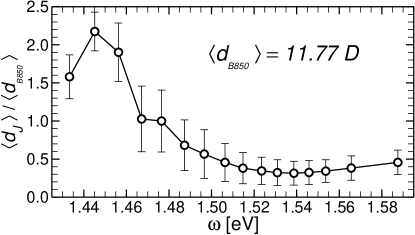
Figure 2: Average transition dipole moments $\langle d_{J}\rangle$ corresponding to the $J=1,\ldots,16$ B850 excitonic states. Both $\langle d_{J}\rangle$ and the corresponding error bars are expressed relative to the mean dipole moment of individual B850s.

The $Q_{y}$ excitations of the truncated BChls were calculated by using Zerner’s semiempirical intermediate neglect of differential overlap method parametrized for spectroscopy (ZINDO/S) within the single-point configuration interaction singles (CIS) approximation Ridley and Zerner (1973); Zerner et al. (1980). Because it is much faster and more accurate than most of the computationally affordable ab initio QC methods (e.g., the Hartree-Fock (HF) CIS method with the minimal STO-3G^∗ basis set), ZINDO/S CIS has been extensively used in the literature to compute low lying optically allowed excited states of pigment molecules Linnanto and Korppi-Tommola (2004); Ihalainen et al. (2001); Linnanto et al. (1999); Damjanovic et al. (2002b). In cases like ours, where thousands of QC calculations are required, the proper balancing between speed and accuracy is absolutely essential. To further increase the computational speed, the active orbital space for the CIS calculations was restricted to the ten highest occupied (HOMO) and the ten lowest unoccupied (LUMO) molecular orbitals. According to previous studies Mercer et al. (1999), as well as our own testings, the choice of a larger active space has negligible effect on the computed Q_y states. Our ZINDO/S calculations were carried out with the QC program packages HyperChemHyperChem, Hypercube, Inc., 1115 NW 4th Street, Gainesville, Florida 32601, USA() (TM) and GAUSSIAN 98Frisch et al. (1998). In each calculation only the lowest four excited states were determined. Only in a small fraction ($<5\%$) of cases was the indentification of the Q_y excited state (characterized by the largest oscillator strength and corresponding to transitions HOMO$\rightarrow$LUMO and HOMO-1$\rightarrow$LUMO+1) problematic requiring careful inspection. We have found that even in such cases the Q_y state had the largest projection of the TDM along the $y$-axis, determined by the $NB$ and $ND$ nitrogen atoms.

The effect of the environment on the quantum system was taken into account through the electric field created by the partial point charges of the environment atoms, including those BChl atoms that were removed during the truncation process. Thus, the dynamics of the nuclear degrees of freedom (described by MD simulation) have a two-fold effect on the fluctuations of the Q_y state, namely they lead to: (1) conformational fluctuation of the (truncated) BChls, and (2) a fluctuating electric field created by the thermal motion of the corresponding atomic partial charges. In order to assess the relative importance of these two effects the time series $\Delta{E}_{n}(t)$ were calculated both in the the presence and in the absence of the point charges. Since the ZINDO/S implementation in GAUSSIAN 98 does not work in the presence of external point charges, these calculations were done with HyperChem. The ZINDO/S calculations without point charges were carried out with both QC programs and yielded essentially the same result. For each case, we have performed a total of 12,000 (500 snapshots $\times$ 24 BChls) ZINDO/S calculations. On a workstation with dual 3GHz Xeon EM64T CPU it took $\sim 2.3$ min/CPU for each calculation with point charges, and only $\sim 0.7$ min/CPU without point charges. Thus, on a cluster of five such workstations, all 24,000 ZINDO/S runs were completed in $\sim 1.9+0.6=2.5$ days.

IV Results and discussion

The time series of the Q_y excitation energies $\Delta{E}_{n}(t_{\ell})$ and TDMs $\mathbf{d}_{n}(t_{\ell})$, ($t_{\ell}=\ell\Delta{t}$; $\ell=0,\ldots,N_{t}$; $N_{t}=499$; $\Delta{t}=2$ fs), were computed with the ZINDO/S CIS method, described in Sec. III.2, for both B850 ($n=1,\ldots,16$ ) and B800 ($n=17,\ldots,24$) BChls in a LH2 ring from Rs. molischianum, using snapshots from the all atom MD simulation described in Sec. III.1. The calculations were done both with and without the point charges of the atoms surrounding the truncated BChls. The $1$ ps long time series appear to be sufficiently long for calculating the DOS of the Q_y excitation energies and the corresponding OD and CD spectra. In Ref. Mercer et al., 1999 it has been found that at least a $2.2$ ps long MD trajectory was needed for proper evaluation of optical observables related to their MD/QC calculations. However, our test calculations showed no significant difference between the energy gap autocorrelation functions calculated from a $2$ ps and a $1$ ps long energy gap time series. Therefore, to reduce the computational time we have opted for the latter.

Figure 3: Absorption spectrum $I_{DOS}(\omega)$ of LH2 for Rs. molischianum calculated as a combined DOS of B800 BChls and B850 excitons weighted by the corresponding dipole strengths (solid line). $I_{DOS}(\omega)$ was blueshifted by $20$ meV in order to overlay its B850 peak with the corresponding one in the experimental OD spectrum Zhang et al. (2000) (dashed line).

IV.1 Energy gap density of states (DOS) and transition dipole moments (TDMs)

Figure 1 shows the Q_y energy gap DOS, $\mathcal{N}(\omega)$, of the individual B800 [top (a) panel] and B850 [bottom (b) panel] BChls calculated, according to Eqs. (6), as normalized binned histograms of the time series $\Delta{E}_{B800}\equiv\Delta{E}_{n}(t_{\ell})$ with $n=17,\ldots,24$, and $\Delta{E}_{B850}\equiv\Delta{E}_{n}(t_{\ell})$ with $n=1,\ldots,16$, respectively. In order to eliminate the noise due to finite sampling, the graphs have been smoothened out by a running average procedure. The same smoothing out procedure has been applied to all subsequent lineshape and spectra calculations. In the absence of the point charge distribution of the environment $\mathcal{N}(\omega)$ for B800 and B850 (dashed lines) are almost identical, having peak position at $1.51$ eV ($817$ nm) and $1.515$ eV ($818$ nm), and full width at half maximum (FWHM) $51$ meV and $59$ meV, respectively. The fact that the peak position practically coincides with the mean energy gap is indicative that the DOS is symmetric with respect to its maximum.

Figure 4: Normalized autocorrelation function $C(t)/C(0)$ of the energy gap fluctuations $\delta{E}(t)=E(t)-\langle E\rangle$ for individual B800 (dashed line) and B850 (solid line) BChls, calculated using Eq. . The mean square energy gap fluctuations are $C_{B800}(0)=3.16\times 10^{-3}~{}\text{eV}^{2}$ and $C_{B850}(0)=8.68\times 10^{-4}~{}\text{eV}^{2}$

It should be noted that essentially the same mean energy gap of $1.5$ eV was obtained in similar MD/QC calculations (i) by us (data not shown) in the case of a truncated BChl-a in vacuum but artificially coupled to a Langevin heat bath at room temperature, and (ii) by Mercel et al. Mercer et al. (1999) for a BChl-a solvated in methanol also at room temperature. Although in case (ii) the width of the DOS appears to be somewhat broader (FWHM$\approx{65}$ eV) than in case (i), for which FWHM$\approx{58}$ meV, based on these results one can safely conclude that the thermal motion of the nuclei in individual BChls lead to Q_y energy gap fluctuations that are insensitive to the actual nature of the nonpolar environment. Since in LH2 from Rs. molischianum the surrounding of the B800s is polar while that of the B850s is not, one expects that once the point charges of the environment are taken into account in the QC calculations $\mathcal{N}(\omega)$ should change dramatically only in the case of B800. Indeed, as shown in Fig. 1b (solid line), in the presence of the point charges the peak of $\mathcal{N}_{B850}(\omega)$ is only slightly red shifted to $1.502$ eV ($825$ nm) and essentially without any change in shape with FWHM$\approx{53}$ meV. By contrast, the DOS for B800 in the presence of the point charges (Fig. 1a) has qualitatively changed. The induced higher energy fluctuations not only spoil the symmetry of $\mathcal{N}_{B800}(\omega)$ but also increase dramatically its broadening, characterized by FWHM$\approx{100}$ meV. Thus, in spite of a small blueshift to $1.528$ eV ($811$ nm) of the peak of $\mathcal{N}_{B800}(\omega)$ the mean value of the energy gap $\langle\Delta{E}_{B800}\rangle=1.556$ eV ($797$ nm) is increased considerably, matching rather well the experimental value of $800$ nm.

The time series of the excitonic energies $\Delta{E}_{J}(t_{\ell})$, $J=1,\ldots,16$, of the B850 BChls were determined by solving for each MD snapshot, within the point-dipole approximation, the eigenvalue equation (16). In calculating the matrix elements (15) $\mathbf{r}_{n}$ was identified with the position vector of the Mg atom in the $n$-th BChl. Consistent with the Condon approximation, the magnitude of the computed B850 TDM time series exhibited a standard deviation of less than 4% about the average value $\langle d_{B850}\rangle=11.77$ D. The latter is by a factor of $k=1.87$ larger than the experimentally accepted $6.3$ D value of the Q_y TDM of BChl-a Visscher et al. (1989). Thus, to account for this overestimate of the TDM by the ZINDO/S CIS method, instead of using a reasonable value of $1.86$ for the relative dielectric constant of the protein environment in Eq. (15) we set for all the calculations reported in this paper $\varepsilon_{r}=6.5\,(=1.86\times 1.87^{2})$. Equivalently, one can rescale all TDMs from the ZINDO/S calculations by the factor $k^{-1}$ and set $\varepsilon_{r}=1.86$. Either way the mean value of the nearest neighbor dipolar coupling energies between B850s were $27$ meV$\approx{220}$ cm^-1 within a protomer and $24$ meV$\approx{196}$ cm^-1 between adjacent heterodimers. Just like in the case of individual BChls, the DOS corresponding to the B850 excitonic energies (Fig. 1b - thick line) was calculated as a binned histogram of $\Delta{E}_{J}(t_{\ell})$. As expected, the excitonic DOS is not sensitive to whether the point charges of the environment are included or not in the B850 site energy calculations.

Figure 5: Spectral density function $J(w)$ for B800 (dashed line) and B850 (solid line) obtained according to Eq. (12).

The mean excitonic TDMs, calculated from Eq. (17) and expressed in terms of $\langle d_{B850}\rangle$, are shown in Fig. 2. The error bars represent the standard deviation of the time series $d_{J}(t_{\ell})$. In agreement with previous studies, most of the dipole strength is amassed into the lowest three excitonic states.

As discussed in Sec. II, a rough estimate of the lineshape function can be obtained as the combined DOS of the B800 BChls and B850 excitons. In this approximation the OD spectrum reads

$$I_{DOS}(\omega)\propto\omega\left[\sum_{J}d_{J}^{2}\langle\delta(\omega-\Delta{E}_{J})\rangle+\sum_{B800}d_{B800}^{2}\langle\delta(\omega-\Delta{E}_{B800})\rangle\right]\;,$$ (23)

where the $B800$ index in the last term means summation over all B800 BChls. Figure 3 shows the calculated $I_{DOS}(\omega)$ blueshifted by $20$ eV (solid line) in order to match the B850 peak position with the one in the experimental OD spectrum Ihalainen et al. (2001); Zhang et al. (2000) (dashed line). While the B850 band and the relative heights of the two peaks in $I_{DOS}(\omega)$ match rather well the experimental data, the position and the broadening of the B800 peak do not. This result clearly shows that in general peak positions in optical spectra may be shifted from the corresponding peak positions in the excitation energy spectrum due to correlation effects between the ground and optically active excited states. The latter may also lead to different line broadening of the corresponding peaks. Thus, it appears that in principle, methods for simulating optical spectra in which the position of the peaks are identified with the computed excitation energies (stick spectrum) are not entirely correct and using instead more sophisticated methods that include quantum correlation effects should be preferred. Such method, based on the cumulant approximation of the lineshape function as described in Sec. II, is used in the next section for calculating the OD spectrum of an LH2 ring from Rs. molischianum.

Figure 6: Lineshape functions $\overline{A}_{B800}(\Delta\omega)$ (dashed line) and $\overline{A}_{B850}(\Delta\omega)$ (solid line).

IV.2 Absorption (OD) spectrum

The key quantity for calculating the lineshape functions of the individual B850 and B800 BChls is the (classical) autocorrelation function $C_{n}(t)=\langle\delta{E}_{n}(t)\delta{E}_{n}(0)\rangle$ of the energy gap fluctuation $\delta{E}_{n}(t)=\Delta{E}_{n}(t)-\langle\Delta{E}_{n}\rangle$ determined from the combined MD/QC calculations. Because the time series $\Delta{E}_{n}(t)$ were too short for a proper evaluation of the ensemble average in the individual $C_{n}(t)$, a single time correlation function $C_{B800}(t)$ [$C_{B850}(t)$] was determined by averaging over all B800 [B850] BChls according to the formula

$$\begin{split}C_{\alpha}(t_{\ell})=\frac{1}{M}\sum_{m}\left[\frac{1}{N_{t}-\ell}\sum_{k=1}^{N_{t}-\ell}\delta{E}_{m}(t_{\ell}+t_{k})\delta{E}_{m}(t_{k})\right]\;,\\ \text{where}\;M=8,\;m=17,\ldots,24\;\;\text{for}\;\;\alpha=B800\;,\\ \text{and}\;M=16,\;m=1,\ldots,16\;\;\text{for}\;\;\alpha=B850\;.\end{split}$$ (24)

The normalized correlation functions $C_{\alpha}(t)/C_{\alpha}(0)$, $\alpha\in\{B800,B850\}$, are plotted in Fig. 4. $C_{\alpha}(0)=\langle\delta{E}^{2}\rangle$ represents the variance of the energy gap fluctuations with $C_{B800}(0)=3.16\times 10^{-3}$ eV² and $C_{B850}(0)=8.68\times 10^{-4}$ eV². The behavior of the two correlation functions is rather similar during the first $150$ fs. Following a sharp decay to negative values in the first $9$ fs, both functions exhibit an oscillatory component of approximately $18.5$ fs period and uneven amplitudes that, in general, are larger for the B800. After $\sim 150$ fs, the autocorrelation functions behave in a distinctive manner, both becoming negligibly small for $t\gtrsim 400$ fs.

Figure 7: Computed (solid line) and experimental (dashed line) absorption spectra (in arbitrary units) of the BChl aggregate in Rs. Molischianum LH2. The computed spectrum has been blue shifted by $20$ meV for best match.

The spectral densities $J_{\alpha}(\omega)$ for B800 and B850, determined according to Eq. (12), are shown in Fig. 5. The prominent peak about $\omega_{p}=0.22$ eV is due to the fast initial decay of $C_{\alpha}(t)$. Being reported in previous studiesMercer et al. (1999); Damjanovic et al. (2002a), by using both ab initio (HF/CIS with STO-3G^∗ basis set) and semi empirical QC methods, these spectral features appear to be intrinsic properties of BChl-a, most likely originating from a strong coupling of the pigment to an intramolecular C$=$O vibronic mode. Often, the environment in a PPC is modeled as an equivalent harmonic (phonon) heat bath for which the cumulant approximation is exact Mukamel (1995). The corresponding phonon spectral density can be written as $J(\omega)=\omega^{2}\sum_{\lambda}g_{\lambda}^{2}\delta(\omega-\omega_{\lambda})$, where $g_{\lambda}$ is the coupling constant to the phonon mode $\lambda$. Thus, one can interpret the magnitude of the spectral functions in Fig. 5 as a measure of the coupling strength to phonons of that particular frequency. The complex structure of the spectral functions indicate that all inter and intra molecular vibronic modes with frequency below $\omega_{p}$ will contribute to the lineshape function. Hence, attempts to use simplified model spectral functions appear to be unrealistic even if these may lead to absorption spectra that match the experimental results.

The lineshape functions of individual B800 and B850, calculated from Eqs. (14), are plotted in Fig. 6. The origin of the frequency axis corresponds to the mean energy gaps $\omega_{B800}$ and $\omega_{B850}$, respectively. The highly polarized surrounding of the B800 BChls in Rs. molischianum renders $A_{B800}(\omega)$ twice as broad (FWHM$\approx{26}$ meV) as $A_{B850}(\omega)$ (FWHM$\approx{13}$ meV). Also, the redshift of the peak of the former ($\Delta\omega\approx 25$ meV) is more than three times larger than that of the latter ($\Delta\omega\approx 7$ meV).

Since the available simulation data is not sufficient to properly estimate the excitonic lineshape functions $A_{J}(\omega)$, by neglecting the effect of exchange narrowing Amerongen et al. (2000); Somsen et al. (1996), we approximated these with $A_{B850}(\omega)$. Thus, the OD spectrum of the LH2 BChls was calculated by using the formula

$$I(\omega)\propto\omega\left[\sum_{J}d_{J}^{2}\overline{A}_{B850}(\omega-\omega_{J})+8d_{B800}^{2}\overline{A}_{B800}(\omega-\omega_{B800})\right]\;,$$ (25)

where $\omega_{J}=\langle\Delta{E}_{J}\rangle$.

As shown in Fig. 7, after an overall blueshift of $20$ meV, $I(\omega)$ matches remarkably well the experimental OD spectrum, especially if we take into account that it was obtained from the sole knowledge of the high resolution crystal structure of LH2 from Rs. molischianum. The reason why both B800 and B850 peaks of $I(\omega)$ are somewhat narrower than the experimental ones is most likely due to the fact that the effect of static disorder is ignored in the present study. Indeed, our calculations were based on a single LH2 ring, while the experimental data is averaged over a large number of such rings. While computationally expensive, in principle, the effect of static disorder could be taken into account by repeating the above calculations for different initial configurations of the LH2 ring and then averaging the corresponding OD spectra.

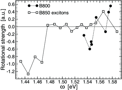
Figure 8: Mean rotational strength of the excitonically coupled B800 (circles) and B850 (rectangles) BChls as a function of the corresponding excitonic energies. The purpose of the thin lines are to guide the eye.

To conclude this section we would like to relate the present work to previous two combined MD/QC studies Mercer et al. (1999); Damjanovic et al. (2002a). In Mercer et al. (1999) it is argued that the ab initio QC method (HF/CIS with the STO-3G^∗ basis set) should be preferred to semi empirical methods for calculating optical spectra because it reproduces better their experimental results. The FWHM of their calculated semi empirical and ab initio absorption spectra of BChl-a in methanol are $\sim{65}$ meV and $\sim{125}$ meV, respectively. These values are similar to the ones we obtained for the same type of calculations for BChl-a in vacuum and in LH2 embedded in its native environment. Since except Ref. Mercer et al., 1999 all experimental results on the Q_y absorption band of BChls we are aware of have a FWHM of $\lesssim{80}$ meV at room temperature, we conclude that in fact the semi empirical ZINDO/S method should be preferable to the ab initio QC method. In general, the latter overestimate the broadening of the OD spectrum by a factor of 2 to 3. In Damjanovic et al. (2002a), the OD spectrum of individual B850s (i.e., without excitonic coupling) calculated with the ab initio method yielded the same FWHM of $\sim{125}$ meV as in Mercer et al. (1999). Once the excitonic coupling was included within the framework of a polaron model, and it was assumed that the entire oscillator strength was carried by a single exciton level of a perfect B850 ring, the FWHM of the resulting OD spectrum was reduced to $\sim{43}$ meV as a result of exchange narrowing. Thus the obtained OD spectrum for the B850s appeared to match rather well the corresponding part of the experimental one. However, by applying the same method to the B800s, where there is no exchange narrowing, the polar environment further broadens the corresponding OD spectrum to a FWHM of $\sim{250}$ meV that is clearly unphysically large. Thus, the conclusion again is that the ZINDO/S CIS semi empirical method should be preferred for calculating optical spectra of PPCs.

IV.3 Circular dichroism (CD) spectrum

Figure 9: (a) CD spectrum contributions due to B800 (dashed line) and B850 (solid line) BChls. (b) Comparison between the computed (solid line) and experimental CD spectrum of the BChl aggregate in Rs. Molischianum LH2.

The CD spectrum of the LH2 BChls from Rs. molischianum was determined by following the theoretical approach described at the end of Sec. II and by employing the same time series (obtained from the combined MD/QC calculations) used for calculating the OD spectrum.

First, the rotational strength of both B850 excitons and B800 BChls were determined by using Eq. (22b). In this equation, just like in the case of the point-dipole interaction matrix elements (15), the vector $\mathbf{r}_{n}$ described the position of the Mg atom in the $n^{th}$ BChl. As already clarified in Sec. II the calculation of the rotational strength of the B800 BChls requires solving the corresponding excitonic Hamiltonian (16) regardless of how small the dipole-dipole coupling is between these BChls. The calculation does not yield either noticeable corrections to the B800 excitation energies or admixture of the corresponding Q_y states, however, it leads to sizable mean rotational strengths as shown in Fig. 8 (filled circles). Similarly to the TDM strengths (Fig. 2), the largest (negative) mean rotational strengths are carried by the four lowest B850 excitonic states as shown in Fig. 8 (open squares). The second highest excitonic state also has a sizable rotational strength and is responsible for enhancing the positive peak of the B800 contribution to the CD spectrum (Fig. 9a).

Second, the CD spectrum is calculated from Eq. (22a) where the summation index $J$ runs over all B850 and B800 excitonic states and $A_{J}(\omega)=\overline{A}_{\alpha}(\omega-\omega_{J})$, with $\alpha\in\{B850,B800\}$. Figure 9a shows the CD spectrum contribution by the B850 (solid line) and B800 (dashed line). Both contributions have the same qualitative structure with increasing energy: a pronounced negative peak followed by a smaller positive one. The B850 negative CD peak is about twice as large as the corresponding B800 peak. The total CD spectrum, given by the superposition of the B850 and B800 contributions, is shown in Fig. 9b (solid line) and matches fairly well the experimental spectrum Ihalainen et al. (2001) (dashed line). It should be emphasized that apart from an overall scaling factor the CD spectrum was calculated from the same MD/QC data as the OD spectrum by following the procedure described above.

V Conclusions

The continuous increase in processor power and availability of high performance computer clusters, along with the growing number of high resolution crystal structures of membrane bound pigment-protein complexes make feasible the theoretical characterization of the spectral and optical properties of such systems at atomic level. By applying an approach that combines all atom MD simulations, efficient semi empirical QC calculations and quantum many-body theory we have shown that starting solely from the atomic structure of the LH2 ring from Rs. molischianum the OD and CD spectra of this PPC can be predicted with reasonable accuracy at affordable computational costs. The configuration snapshots taken with femtosecond frequency during the MD simulation of the PPC in its native, fully solvated lipid-membrane environment at room temperature and normal pressure provide the necessary input for the QC calculations of the optical excitation energies and transition dipole moments of the pigment molecules. The obtained time series are used to evaluate within the second cumulant approximation the optical lineshape functions as the Fourier transform of the quantum dipole-dipole correlation function. Our choice of the ZINDO/S CIS method for the QC calculations was motivated by the fact that it is almost two orders of magnitude faster and much more accurate than the most affordable ab initio method (HF/CIS with the STO-3G^∗ basis set). Compared to the former, the latter method overestimates by a factor of 2 to 3 both the excitation energies and the broadening of the energy spectrum. Just like in several previous studies Linnanto and Korppi-Tommola (2004); Ihalainen et al. (2001); Linnanto et al. (1999); Damjanovic et al. (2002b), we have found that the ZINDO/S method repeatedly yields results in good agreement with existing experimental data.

By investigating the excitation energy spectrum of the LH2 BChls both in the presence and in the absence of the atomic partial charges of their environment we have convincingly demonstrated that the large broadening of the B800 peak is due primarily to the electric field fluctuations created by the polar surrounding environment of the B800s. There is no such effect for the B850s which sit in a nonpolar local environment. The broadening of the B850 peak is due to the sizable excitonic coupling between these BChls. Since only the lowest three excitonic states carry most of the available dipole strength, in spite of the $\sim{0.2}$ eV wide excitonic band, the B850 absorption peak has a FWHM only slightly larger than the B800 one.

It is rather remarkable that both the OD and the CD spectra of the considered LH2 complex are fairly well predicted by our combined MD/QC method. However, a more thorough testing of the proposed method, involving other PPCs is necessary to fully establish its capability of predicting optical properties by using only atomic structure information.

References

- Renger et al. (2001) T. Renger, V. May, and O. Kuhn, Phys. Rep.-Rev. Sec. Phys. Lett. 343, 138 (2001).
- Chernyak et al. (1998) V. Chernyak, W. M. Zhang, and S. Mukamel, J. Chem. Phys. 109, 9587 (1998).
- Mukamel (1995) S. Mukamel, Principles of nonlinear optical spectroscopy (Oxford University Press, New York, 1995).
- May and Kühn (2000a) V. May and O. Kühn, Charge and Energy Transfer Dynamics in Molecular Systems (WILEY-VCH, Berlin, 2000a).
- van Amerongen et al. (2000) H. van Amerongen, L. Valkunas, and R. van Grondelle, Photosynthetic Excitons (World Scientific, Singapore, 2000).
- Koepke et al. (1996) J. Koepke, X. C. Hu, C. Muenke, K. Schulten, and H. Michel, Structure 4, 581 (1996).
- McDermott et al. (1995) G. McDermott, S. Prince, A. Freer, A. Hawthornthwaite-Lawless, M. Papiz, R. Cogdell, and N. Isaacs, Nature 374, 517 (1995).
- Hu et al. (2002) X. Hu, T. Ritz, A. Damjanovic, F. Autenrieth, and K. Schulten, Q Rev Biophys 35, 1 (2002).
- Yang et al. (2001) M. Yang, R. Agarwal, and G. R. Fleming, J. Photochem. Photobiol. A-Chem. 142, 107 (2001).
- Sundstrom et al. (1999) V. Sundstrom, T. Pullerits, and R. van Grondelle, J. Phys. Chem. B 103, 2327 (1999).
- Wu et al. (1997) H. M. Wu, M. Ratsep, R. Jankowiak, R. J. Cogdell, and G. J. Small, J. Phys. Chem. B 101, 7641 (1997).
- Beekman et al. (1997) L. M. P. Beekman, R. N. Frese, G. J. S. Fowler, R. Picorel, R. J. Cogdell, I. H. M. vanStokkum, C. N. Hunter, and R. vanGrondelle, J. Phys. Chem. B 101, 7293 (1997).
- Georgakopoulou et al. (2002) S. Georgakopoulou, R. N. Frese, E. Johnson, C. Koolhaas, R. J. Cogdell, R. van Grondelle, and G. van der Zwan, Biophys. J. 82, 2184 (2002).
- Somsen et al. (1996) O. J. G. Somsen, R. vanGrondelle, and H. vanAmerongen, Biophys. J. 71, 1934 (1996).
- Scholes and Fleming (2000) G. D. Scholes and G. R. Fleming, J. Phys. Chem. B 104, 1854 (2000).
- Damjanovic et al. (2002a) A. Damjanovic, I. Kosztin, U. Kleinekathofer, and K. Schulten, Phys Rev E Stat Nonlin Soft Matter Phys 65, 031919 (2002a).
- He et al. (2002) Z. He, V. Sundstrom, and T. Pullerits, J. Phys. Chem. B 106, 11606 (2002).
- Hu et al. (1998a) X. Hu, A. Damjanovic, T. Ritz, and K. Schulten, Proc. Natl. Acad. Sci. USA 95, 5935 (1998a).
- Ihalainen et al. (2001) J. A. Ihalainen, J. Linnanto, P. Myllyperkio, I. H. M. van Stokkum, B. Ucker, H. Scheer, and J. E. I. Korppi-Tommola, J. Phys. Chem. B 105, 9849 (2001).
- Linnanto et al. (1999) J. Linnanto, J. E. I. Korppi-Tommopa, and V. M. Helenius, J. Phys. Chem. B 103, 8739 (1999).
- Meier et al. (1997) T. Meier, Y. Zhao, V. Chernyak, and S. Mukamel, J. Chem. Phys. 107, 3876 (1997).
- Ray and Makri (1999) J. Ray and N. Makri, J. Phys. Chem. A 103, 9417 (1999).
- Jang and Silbey (2003) S. J. Jang and R. J. Silbey, J. Chem. Phys. 118, 9324 (2003).
- Hu and Schulten (1997) X. Hu and K. Schulten, Physics Today 50, 28 (1997).
- Hu et al. (1998b) X. Hu, A. Damjanović, T. Ritz, and K. Schulten, Proc. Natl. Acad. Sci. USA 95, 5935 (1998b).
- Zhang et al. (2000) J.-P. Zhang, R. Fujii, P. Qian, T. Inaba, T. Mizoguchi, and Y. Koyama, J. Phys. Chem. B 104, 3683 (2000).
- Amerongen et al. (2000) H. v. Amerongen, L. Valkunas, and R. v. Grondelle (2000).
- Mercer et al. (1999) I. Mercer, I. Gould, and D. Klug, J. Phys. Chem. B 103, 7720 (1999).
- May and Kühn (2000b) V. May and O. Kühn, Charge and Energy Transfer Dynamics in Molecular Systems (WILEY-VCH, Berlin, 2000b).
- Makri (1999) N. Makri, J. Phys. Chem. B 103, 2823 (1999).
- Schulten and Tesch (1991) K. Schulten and M. Tesch, Chem. Phys. 158, 421 (1991).
- Egorov et al. (1999) S. A. Egorov, K. F. Everitt, and J. L. Skinner, J. Phys. Chem. A 103, 9494 (1999).
- MacKerell Jr. et al. (1992) A. D. MacKerell Jr., D. Bashford, M. Bellott, et al., FASEB J. 6, A143 (1992).
- MacKerell Jr. et al. (1998) A. D. MacKerell Jr., D. Bashford, M. Bellott, et al., J. Phys. Chem. B 102, 3586 (1998).
- Schlenkrich et al. (1996) M. Schlenkrich, J. Brickmann, A. D. MacKerell Jr., and M. Karplus, in Biological Membranes: A Molecular Perspective from Computation and Experiment, edited by K. M. Merz and B. Roux (Birkhauser, Boston, 1996), pp. 31–81.
- Jorgensen et al. (1983) W. L. Jorgensen, J. Chandrasekhar, J. D. Madura, R. W. Impey, and M. L. Klein, J. Chem. Phys. 79, 926 (1983).
- Feller et al. (1995) S. E. Feller, Y. H. Zhang, R. W. Pastor, and B. R. Brooks, J. Chem. Phys. 103, 4613 (1995).
- Darden et al. (1993) T. Darden, D. York, and L. Pedersen, J. Chem. Phys. 98, 10089 (1993).
- Phillips et al. (2005) J. C. Phillips, R. Braun, W. Wang, J. Gumbart, E. Tajkhorshid, E. Villa, C. Chipot, R. D. Skeel, L. Kale, and K. Schulten, Journal of Computational Chemistry 26, 1781 (2005).
- Miyamoto and Kollman (1992) S. Miyamoto and P. A. Kollman, J. Comp. Chem. 13, 952 (1992).
- Cory et al. (1998) M. G. Cory, M. C. Zerner, X. Hu, and K. Schulten, J. Phys. Chem. B 102, 7640 (1998).
- Ridley and Zerner (1973) J. Ridley and M. Zerner, Theor. Chim. Acta 32, 111 (1973).
- Zerner et al. (1980) M. Zerner, G. Loew, R. Kirchner, and U. J. Mueller-Westerhoff, Am. Chem. Soc. 102, 589 (1980).
- Linnanto and Korppi-Tommola (2004) J. Linnanto and J. Korppi-Tommola, J Comput Chem 25, 123 (2004).
- Damjanovic et al. (2002b) A. Damjanovic, H. M. Vaswani, P. Fromme, and G. R. Fleming, J. Phys. Chem. B 106, 10251 (2002b).
- HyperChem, Hypercube, Inc., 1115 NW 4th Street, Gainesville, Florida 32601, USA() (TM) HyperChem(TM), Hypercube, Inc., 1115 NW 4th Street, Gainesville, Florida 32601, USA.
- Frisch et al. (1998) M. J. Frisch, G. W. Trucks, H. B. Schlegel, G. E. Scuseria, M. A. Robb, J. R. Cheeseman, J. A. M. V. G. Zakrzewski, R. E. Stratmann, J. C. Burant, J. M. M. S. Dapprich, et al., Gaussian 98, Gaussian Inc., Pittsburgh, PA (1998).
- Visscher et al. (1989) K. Visscher, H. Bergstrom, V. Sundström, C. Hunter, and R. van Grondelle, Photosynth. Res. 22, 211 (1989).