Convergence of CI single center calculations of positron-atom interactions

Abstract

The Configuration Interaction (CI) method using orbitals centered on the nucleus has recently been applied to calculate the interactions of positrons interacting with atoms. Computational investigations of the convergence properties of binding energy, phase shift and annihilation rate with respect to the maximum angular momentum of the orbital basis for the $e^{+}$Cu and PsH bound states, and the $e^{+}$-H scattering system were completed. The annihilation rates converge very slowly with angular momentum, and moreover the convergence with radial basis dimension appears to be slower for high angular momentum. A number of methods of completing the partial wave sum are compared, an approach based on a $\Delta X_{J}=a(J+{\scriptstyle\frac{1}{2}})^{-n}+b(J+{\scriptstyle\frac{1}{2}})^{-(n+1)}$ form (with $n=4$ for phase shift (or energy) and $n=2$ for the annihilation rate) seems to be preferred on considerations of utility and underlying physical justification.

I Introduction

In the last few years there have been a number of calculations of positron-binding to atoms Mitroy and Ryzhikh (1999); Dzuba et al. (1999, 2000); Bromley et al. (2000); Bromley and Mitroy (2002a, b, c, d); Saito (2003a, b, 2005) and positron-scattering from atoms and ions Bromley and Mitroy (2003); Novikov et al. (2004); Gribakin and Ludlow (2004) using orthodox CI type methods with large basis sets of single center orbitals. Besides the calculations on atoms, there have some attempts to calculate the properties of positrons bound to molecules with modified versions of standard quantum chemistry methods Tachikawa et al. (2003); Strasburger (2004); Buenker et al. (2005).

One feature common to all these CI type calculations is the slow convergence of the binding energy, and the even slower convergence of the annihilation rate. The attractive electron-positron interaction leads to the formation of a Ps cluster (i.e. something akin to a positronium atom) in the outer valence region of the atom Ryzhikh et al. (1998); Dzuba et al. (1999); Mitroy et al. (2002); Saito (2003a). The accurate representation of a Ps cluster using only single particle orbitals centered on the nucleus requires the inclusion of orbitals with much higher angular momenta than a roughly equivalent electron-only calculation Strasburger and Chojnacki (1995); Schrader (1998); Mitroy and Ryzhikh (1999); Dzuba et al. (1999). For example, the largest CI calculations on PsH and the group II positronic atoms have typically involved single particle basis sets with 8 radial functions per angular momenta, $\ell$, and inclusion of angular momenta up to $\ell_{\rm max}=10$ Bromley and Mitroy (2002a, b); Saito (2003a). Even with such large basis sets, between 5-60$\%$ of the binding energy and some 30-80$\%$ of the annihilation rate were obtained by extrapolating from the $\ell_{\rm max}=10$ to the $\ell_{\rm max}=\infty$ limit.

Since our initial CI calculations on group II and IIB atoms Bromley and Mitroy (2002a, b, c), advances in computer hardware mean larger dimension CI calculations are possible. In addition, program improvements have removed the chief memory bottleneck that previously constrained the size of the calculation. As a result, it is now appropriate to revisit these earlier calculation to obtain improved estimates of the positron binding energies and other expectation values. However, as the calculations are increased in size, it has become apparent that the issue of slow convergence of the physical observables with the angular momenta of the basis orbitals is the central technical issue in any calculation.

Whilst it is desirable to minimize the amount of mechanical detail in any discussion (so as not to distract from the physics), the ability to draw reliable conclusions from any calculation depends crucially on the treatment of the higher partial waves. For example, the treatment of the higher partial waves in separate calculations by Saito Saito (2005) has already been shown to be flawed Mitroy and Bromley (2005) while the present work exposes the defects in the methods of Gribakin and Ludlow Gribakin and Ludlow (2004). The present work, therefore, is solely devoted to an in-depth examination of the convergence properties of mixed electron-positron calculations.

In our previous works, Bromley and Mitroy (2002a, b, c, 2003); Novikov et al. (2004), a relatively simple solution to this problem was adopted. In effect, it was assumed that the successive increments to any observable scaled as an inverse power series in $\ell_{\rm max}$. This approach does have limitations as do the approaches adopted by other groups Saito (2003b, 2005); Gribakin and Ludlow (2004); Mitroy and Bromley (2005). In the present article, we examine the convergence properties of positron binding calculations upon PsH and $e^{+}$Cu, and a positron scattering calculation upon the $e^{+}$-H system with respect to angular momentum and the dimension of the radial basis sets. The limitations of existing calculations are exhibited, and some improved prescriptions for estimating the variational limit are introduced and tested.

II Existing methods of performing the angular momentum extrapolation

II.1 The nature of the problem

The positron-atom wave function is written as a linear combination of states created by multiplying atomic states to single particle positron states with the usual Clebsch-Gordan coupling coefficients ;

$$|\Psi;LS\rangle = \sum_{i,j}c_{i,j}\ \langle L_{i}M_{i}\ell_{j}m_{j}|LM_{L}\rangle\langle S_{i}M_{S_{i}}{\scriptstyle\frac{1}{2}}\mu_{j}|SM_{S}\rangle$$ (1)

$$\times \ \Phi_{i}(Atom;L_{i}S_{i})\phi_{j}({\bf r}_{0})\ .$$

In the case of a single electron system, e.g. H, $\Phi_{i}(Atom;L_{i}S_{i})$ is just a single electron wave function, i.e. an orbital. For a di-valent system, $\Phi_{i}(Atom;L_{i}S_{i})$ is an antisymmetric product of two single electron orbitals coupled to have good $L_{i}$ and $S_{i}$ quantum numbers. The function $\phi_{j}({\bf r}_{0})$ is a single positron orbital. The single particle orbitals are written as a product of a radial function and a spherical harmonic:

$$\phi({\bf r})=P(r)Y_{\ell m}({\hat{\bf r}})\ .$$ (2)

The radial wave functions are a linear combination of Slater Type Orbitals (STO) Mitroy (1999) and Laguerre Type Orbitals (LTOs). Most of the time the radial functions are LTOs, the exceptions occurring for single electron states with angular momenta equal to those of any occupied core orbitals. Since the Hartree-Fock core orbitals are written as a single combination of STOs, some of the active electron basis is written as linear combinations of STOs before the switch to a LTO basis is made. The LTO basis Bromley and Mitroy (2002a, b) has the property that the basis can be expanded toward completeness without having any linear independence problems.

The present discussion is specific to positronic systems with a total orbital angular momentum of zero. It is straight-forward to generalize the discussion to states with $L>0$, but this just adds additional algebraic complexities without altering any of the general conclusions.

For a one electron system, the basis can be characterized by the index $J$, the maximum orbital angular momentum of any single electron or single positron orbital included in the expansion of the wave function.

For two electron systems, the $L=0$ configurations are generated by letting the two electrons and positron populate the single particle orbitals subject to two selection rules,

$$\max(\ell_{0},\ell_{1},\ell_{2}) \leq J\ ,$$ (3)

$$\min(\ell_{1},\ell_{2}) \leq L_{\rm int}\ .$$ (4)

In these rules $\ell_{0}$ is the positron orbital angular momentum, while $\ell_{1}$ and $\ell_{2}$ are the angular momenta of the electrons. The maximum angular momentum of any electron or positron orbital included in the CI expansion is $J$. The other parameter, $L_{\rm int}$ is used to eliminate configurations involving the simultaneous excitation of both electrons into high $\ell$ states. Double excitations of the two electrons into excited orbitals are important for taking electron-electron correlations into account, but the electron-electron correlations converge a lot more quickly with $L_{\rm int}$ than electron-positron correlations do with $J$. Calculations of the positronic bound states of the group II atoms and PsH Bromley and Mitroy (2002a, b) showed that the annihilation rate changed by less than 1$\%$ when $L_{\rm int}$ was varied from 1 to 3. The present set of calculations upon PsH were performed with $L_{\rm int}=4$. Further details about the methods used to perform the calculations can be found elsewhere Bromley and Mitroy (2002a, b).

Various expectation values are computed to provide information about the structure of these systems. All observable quantities can be defined symbolically as

$$\langle X\rangle^{J}=\sum_{L=0}^{J}\Delta X^{L}\ ,$$ (5)

where $\Delta X^{J}$ is the increment to the observable that occurs when the maximum orbital angular momentum is increased from $J\!-\!1$ to $J$, e.g.

$$\Delta X^{J}=\langle X\rangle^{J}-\langle X\rangle^{J-1}\ .$$ (6)

Hence, one can write formally

$$\langle X\rangle^{\infty}=\langle X\rangle^{J}+\sum_{L=J+1}^{\infty}\Delta X^{L}\ .$$ (7)

The first term on the right hand side will be determined by explicit computation while the second term must be estimated. The problem confronting all single center calculations is that most expectation values, $\langle X\rangle^{J}$ converges relatively slowly with $J$ and so the contribution of the second term can be significant. A sensible working strategy is to make $J$ as large as possible while simultaneously trying to use the best possible approximation to mop-up the rest of the partial wave sum.

II.2 Existing extrapolation techniques and their limitations

One of the first groups to confront this issue and attempt a solution was the York University group of McEachran and Stauffer. They performed a series of polarized orbital calculations of positron scattering from rare gases McEachran et al. (1978a, b); McEachran et al. (1979, 1980). The decrease in energy when the target atom relaxed in the field of a fixed positron was used to determine the polarization potential as a function of the distance from the nucleus. The polarized orbital method implicitly includes the influence of virtual Ps formation (within an adiabatic approximation), and this means that slow convergence can be expected. McEachran and Stauffer found that the scattering observables, namely the phase shift, and the $Z_{\rm eff}$ annihilation parameter, converged slowly with $J$, the largest angular momentum of the polarized electron orbital set used to represent the adjustment of the atomic charge cloud in the field of the positron. They took this into consideration by assuming their polarization potential scaled as $J^{-p}$ and the polarized orbital scaled as $J^{-q}$ at large $J$. They found $p\approx 3.8$ and $q\approx 1.8$ for the rare gases at $J\approx 12$.

The recent CI-type calculations of Mitroy and collaborators also used an inverse power relation of $J^{-p}$, to complete the partial wave sum Bromley and Mitroy (2002a, b, 2003). In this case, the observables, $\varepsilon^{J}$, $\delta^{J}$, $\Gamma^{J}$ and $Z^{J}_{\rm eff}$ were extrapolated. This contrasts with the polarized orbital calculations where the polarization potential and polarized orbital were extrapolated. The value of $p$ was given by

$$p=\ln\left(\frac{\Delta X^{J-1}}{\Delta X^{J}}\right)\biggl{/}\ln\left(\frac{J-1}{J}\right)\ ,$$ (8)

while the constant factor is

$$A_{X}=\Delta X^{J}J^{p}\ .$$ (9)

The correction factor was then evaluated by doing the sum $\sum_{L=J+1}^{\infty}A_{X}/L^{p}$ explicitly with an upper limit in the thousands.

Gribakin and Ludlow Gribakin and Ludlow (2002) applied perturbation theory and the ideas of Schwartz Schwartz (1962a, b) to determine the asymptotic behavior of the partial wave increments to the binding energies, phase shifts and annihilation rates of positron-atom systems. This work is largely derived from previous work on the partial wave expansion of two electron atoms Hill (1985); Kutzelnigg and Morgan III (1992); Schmidt and Linderberg (1993); Ottschofski and Kutzelnigg (1997). They determined that the binding energy $E$, annihilation rate $\Gamma$, phase shift $\delta$, and collisional annihilation parameter $Z_{\rm eff}$ obey

$$\Delta E^{J}=\langle E\rangle^{J}-\langle E\rangle^{J-1} \sim \frac{B_{E}}{(J+{\scriptstyle\frac{1}{2}})^{4}}$$ (10)

$$\Delta\Gamma^{J}=\langle\Gamma\rangle^{J}-\langle\Gamma\rangle^{J-1} \sim \frac{B_{\Gamma}}{(J+{\scriptstyle\frac{1}{2}})^{2}}$$ (11)

$$\Delta\delta^{J}=\langle\delta\rangle^{J}-\langle\delta\rangle^{J-1} \sim \frac{B_{\delta}}{(J+{\scriptstyle\frac{1}{2}})^{4}}$$ (12)

$$\Delta Z^{J}_{\rm eff}=\langle Z_{\rm eff}\rangle^{J}-\langle Z_{\rm eff}\rangle^{J-1} \sim \frac{B_{Z}}{(J+{\scriptstyle\frac{1}{2}})^{2}}$$ (13)

These expressions are merely the leading order terms of a series of the form

$$\Delta X^{J}=\frac{B_{X}}{(J+{\scriptstyle\frac{1}{2}})^{n}}+\frac{C_{X}}{(J+{\scriptstyle\frac{1}{2}})^{n+1}}+\ldots$$ (14)

To perform the actual extrapolation during a calculation of positron-hydrogen scattering, Gribakin and Ludlow Gribakin and Ludlow (2004) did a fit to calculated values at $J=9$ and $J=10$ with the formulae

$$\delta=\langle\delta\rangle^{\infty} = \langle\delta\rangle^{J}+\sum_{L=J+1}^{\infty}\frac{B_{\delta}}{(L+{\scriptstyle\frac{1}{2}})^{4}}$$ (15)

$$\approx \langle\delta\rangle^{J}+\frac{B_{\delta}}{3(J+{\scriptstyle\frac{1}{2}})^{3}}\ \ ,$$

$$Z_{\rm eff}=\langle Z_{\rm eff}\rangle^{\infty} = \langle Z_{\rm eff}\rangle^{J}+\sum_{L=J+1}^{\infty}\frac{B_{Z}}{(L+{\scriptstyle\frac{1}{2}})^{2}}$$ (16)

$$\approx \langle Z_{\rm eff}\rangle^{J}+\frac{B_{Z}}{J+{\scriptstyle\frac{1}{2}}}\ ,$$

and so determined $Z_{\rm eff}$ and $\delta$. They used the approximate identities in eqs. (15) and (16) rather than explicitly evaluating the infinite sum. The identities appear to have been derived as an approximation to the $\int^{\infty}_{J+1}(L+{\scriptstyle\frac{1}{2}})^{-2}\ dL$ integral. However, in equating the sum to the integral they implicitly assume a rectangle rule representation of the integral which is in error of 5-10$\%$ for $J\in[7,10]$ (the net effect of this is that Gribakin and Ludlow state that the increments decrease as $B/(L+{\scriptstyle\frac{1}{2}})^{n}$ but actually assume a $B/L^{n}$ decrease when evaluating the $J\to\infty$ correction). A better approximation to the series is obtained by using a mid-point rule to represent the integral. Doing this leads to

$$\sum_{L=J+1}^{\infty}\frac{1}{(L+{\scriptstyle\frac{1}{2}})^{n}}\approx\frac{1}{(n-1)(J+1)^{n-1}}\ .$$ (17)

This approximation is accurate to 0.1$\%$ for $n=2$ and $J=7$.

It will be shown that a more serious problem with the Gribakin and Ludlow methodology is that eqs. (15) and (16) cannot reveal whether the calculated $Z^{J}_{\rm eff}$ are deviating from the expected asymptotic form. For example, successive increments to either the phase shift or $Z_{\rm eff}$ have usually decreased more slowly with $J$ (for $J$ ranging between 10 and 18) than indicated by eqs. (10)-(13) Bromley and Mitroy (2002a, b, 2003); Novikov et al. (2004). Instead of having $p=2$ or $p=4$ the successive increments often gave slightly smaller values for $p$. The approach adopted by Gribakin and Ludlow is insensitive to these deviations.

Saito has investigated the structure of the PsH and the Ps-halogen systems with the CI method Saito (2003a, 2005). A Natural Orbital (NO) truncation algorithm based on the energy was used to reduce the dimensionality of the secular equations, thus making calculations on the heavier halogen atoms viable. Besides using the inverse power series, Saito used the functional form

$$\Delta X^{J}=10^{-\alpha(\log_{10}J)^{\beta}+\gamma}\ ,$$ (18)

to complete the partial wave sum for the annihilation rate. This function was not based on any physical principles, and its usage was justified on the grounds that the increments were decreasing faster than $J^{-2}$. However, it has been suggested that the annihilation rate increments were decreasing too quickly because the dimension of the radial basis used in the Ps-halogen calculations was simply too small Mitroy and Bromley (2005). So the rationale behind the usage of eq. (18) is questionable.

Some mention must be made of the difficulties associated with the slower convergence of the annihilation rate. Consider the PsH system, a calculation with $J=9$ gave 72$\%$ of the total annihilation rate Bromley and Mitroy (2002a). If one doubled the size of $J$, then eq. (11) suggests that the explicit calculation would only recover 86$\%$ of the total annihilation rate. And it would take a calculation with $J\approx 250$ to recover 99$\%$ of the annihilation rate. The situation is even more sobering when one considers that the annihilation rate converges faster for PsH (since it is the most compact) than for any other positron binding system.

III Comparison of existing and new approaches to the partial wave extrapolation

III.1 The different alternatives

In order to expose the strengths and deficiencies of existing approaches, very large calculations have been performed on three mixed electron-positron systems. These are the $e^{+}$-H scattering system for the $\ell=0$ partial wave, and the bound PsH and $e^{+}$Cu systems. It will be seen that the typical calculations on these real-world systems do not agree perfectly with the leading order asymptotic form given by Gribakin and Ludlow, i.e. eqs. (10) - (13). Accordingly, six different extrapolation methods for determining the $J\to\infty$ correction were tested. These were:

Method $p$. The successive increments to all quantities are assumed to obey an

$$X^{J}=\frac{A_{X}}{(J+{\scriptstyle\frac{1}{2}})^{p}}\ ,$$ (19)

law with the exponent $p$ determined from eq. (20). The value of $p$ derived from three successive calculation of $X^{J-2}$,$X^{J-1}$ and $X^{J}$ is given by

$$p=\ln\left(\frac{\Delta X^{J-1}}{\Delta X^{J}}\right)\biggl{/}\ln\left(\frac{J+{\scriptstyle\frac{1}{2}}}{J-{\scriptstyle\frac{1}{2}}}\right)\ .$$ (20)

(Note, in previous works we have used a $J^{-p}$ series Mitroy and Ryzhikh (1999); Bromley and Mitroy (2002a, b, 2003)). The notations $p_{E}$, $p_{\Gamma}$, $p_{\delta}$ and $p_{Z}$ are used to denote the exponents derived from the partial wave expansions of the energy, annihilation rate, phase shift and $Z_{\rm eff}$ The discrete sum over $L$ in (7) is done explicitly up to $J=200$. The remainder of the sum is then estimated using eq. (17).

Method $p_{\mathrm{av}}$. This is based on Method $p$. Three successive calculations for $(J\!-\!2)$, $(J\!-\!1)$ and $J$ are once again used with eqs. (19) and (20) to determine an initial estimate of $p_{0}$. Then, $p$ is set to the average of $p_{0}$ and the expected value of either 2 or 4. This method makes an admittedly crude attempt to correct method $p$ in those cases where $p_{\delta}$ and $p_{Z}$ were significantly different from 4 and 2 Bromley and Mitroy (2002b). Once $p$ has been fixed, eq. (19) can then be used to determine $A_{X}$ and the discrete sum over $L$ in (7) is done explicitly up to $J=200$. The remainder of the sum is then estimated using eq. (17).

Method GL. The relations eq. (15) and (16) are assumed to be exact. The two largest values of $\langle X\rangle^{J}$ are used to determine $\langle Z_{\rm eff}\rangle^{\infty}$ and $\langle\delta\rangle^{\infty}$. This method mimics the procedure adopted by Gribakin and Ludlow Gribakin and Ludlow (2004).

Method I. The functional form

$$\Delta X^{J}=\frac{B_{X}}{(J+{\scriptstyle\frac{1}{2}})^{n}}$$ (21)

is assumed to apply and the $\Delta X^{J}$ increment are used to determine $B_{X}$. The exponent $n$ is set to $2$ for the annihilation rate and $4$ for the energy or phase shift. The discrete sum over $L$ in (7) is done explicitly up to $J=200$ and beyond that point eq. (17) is used. This method has similarities with the GL method.

Method II. The functional form

$$\Delta X^{J}=\frac{B_{X}}{(J+{\scriptstyle\frac{1}{2}})^{n}}+\frac{C_{X}}{(J+{\scriptstyle\frac{1}{2}})^{n+1}}\ ,$$ (22)

is assumed to apply and the $\Delta X^{J}$ and $\Delta X^{J-1}$ increments are used to determine $B_{X}$ and $C_{X}$. The second term in eq. (22) comes from 3rd-order perturbation theory Hill (1985); Kutzelnigg and Morgan III (1992); Ottschofski and Kutzelnigg (1997). The exponent $n$ is set to $2$ for the annihilation rate and $4$ for the energy or phase shift. The discrete sum over $L$ in (7) is done explicitly up to $J=200$ and beyond that point eq. (17) is used.

Method III. The functional form

$$\Delta X^{J}=\frac{B_{X}}{(J+{\scriptstyle\frac{1}{2}})^{n}}+\frac{C_{X}}{(J+{\scriptstyle\frac{1}{2}})^{n+1}}+\frac{D_{X}}{(J+{\scriptstyle\frac{1}{2}})^{n+2}}\ ,$$ (23)

is assumed to apply and the $\Delta X^{J}$, $\Delta X^{J-1}$ and $\Delta X^{J-2}$ increments are used to determine $B_{X}$, $C_{X}$ and $D_{X}$. Other particulars are the same as those for Methods I and II.

Method S. The functional form adopted by Saito, eq. (18) is used. The parameters $\alpha$, $\beta$ and $\gamma$ are determined from $\Delta X^{J-2}$, $\Delta X^{J-1}$ and $\Delta X^{J}$. Then the series is completed by summing to $J=2000$.

III.2 The $e^{+}$-H scattering system

The CI-Kohn method has already been used to generate phase shift and annihilation parameter data for the $e^{+}$-H scattering system Bromley and Mitroy (2003). New calculations with a radial basis set (i.e. the number of LTOs per $\ell$) of increased dimensionality have been done in order to minimize the influence of the radial basis upon any conclusions that are drawn. The present investigation examines $s$-wave $e^{+}$H scattering at $k=0.4\ \ a_{0}^{-1}$.

Table 1: Results of CI-Kohn calculations for $s$-wave $e^{+}$-H scattering at $k=0.4\ \ a_{0}^{-1}$. The variational and close-coupling data in the last three rows are taken from calculations which have basis functions which explicitly depend on the electron-positron distance. The $J\rightarrow\infty$ limits were taken at $J=12$ using the various extrapolation methods as described in the text. The value of $p$ were determined at $J=12$ using eq. (20). The previous CI-Kohn estimates Bromley and Mitroy (2003) include the $J\to\infty$ correction as determined at that time.

$J$	$\langle\delta\rangle^{J}$ (radians)	$\langle Z_{\rm eff}\rangle^{J}$
0	-0.1992097664	0.4529537597
1	-0.01002215705	1.018467362
2	0.05339800596	1.466777767
3	0.08175604707	1.798430751
4	0.09626735469	2.043817341
5	0.1043829191	2.228559914
6	0.1092338304	2.370688616
7	0.1122907225	2.482386967
8	0.1143023638	2.571897852
9	0.1156750002	2.644890677
10	0.1166408472	2.705331457
11	0.1173386269	2.756059864
12	0.1178543969	2.799146079
$J\rightarrow\infty$ limits
$p$	3.6248	1.9583
Method $p$	0.1200652	3.34020
Method $p_{av}$	0.1199020	3.32823
Method GL	0.1196691	3.29464
Method I	0.1197593	3.31675
Method II	0.1199484	3.32750
Method III	0.1199456	3.30092
Method S	0.1198834	3.21989
Other calculations
CI-Kohn $J\rightarrow\infty$ Bromley and Mitroy (2003)	0.1198	3.232
Optical potential Bhatia et al. (1971, 1974)	0.1201	3.327
Variational Van Reeth and Humberston (1997, 1998); Gribakin and Ludlow (2004)	0.1198	3.407
Close Coupling Mitroy and Ratnavelu (1995); Ryzhikh and Mitroy (2000)	0.1191	3.332

The largest calculation for $e^{+}$-H included a minimum of 30 LTOs per $\ell$ with additional LTOs included at small $\ell$. Special attention was given to the $\ell=1$ positron basis since this channel is responsible for the long-range polarization potential. The dimension of the LTO basis was 80 in this case. All radial integrations were taken to 729 $a_{0}$ on a composite Gaussian grid. The earlier calculations of Bromley and Mitroy Bromley and Mitroy (2003) with a minimum of 17 LTOs per $\ell$ will be presented for comparison. Table 1 gives the $e^{+}$-H phase shift and $Z_{\rm eff}$ for $s$-wave scattering at $k=0.4$ $a_{0}^{-1}$ up to $J=12$. The larger basis will be referred to as basis 2 while the older basis will be named basis 1.

First of all, the values of $p_{\delta}$ and $p_{Z}$ derived from the earlier Bromley and Mitroy (2003) and present CI-Kohn calculations are shown together in Figure 1 as a function of $J$. This figure tests whether eqs. (12) and (13) describe the behavior of a real-world calculation.

Figure 1: The exponents $p_{\delta}$ and $p_{Z}$ as a function of $J$ for 2 different CI-Kohn calculations of $s$-wave $e^{+}$-H scattering at $k=0.4\ a_{0}^{-1}$. The short curve labeled GL was plotted using $\langle Z_{\rm eff}\rangle^{J}$ data of GL Gribakin and Ludlow (2004).

Neither $p_{\delta}$ or $p_{Z}$ are within 1$\%$ of the expected asymptotic value at $J=12$ and both are approaching the expected asymptotic limit from below. The two calculations give almost exactly the same $p_{\delta}$ while the larger calculation tends to give smaller values of $p_{Z}$ with the difference becoming greater as $J$ increases. The increasing difference between $p_{Z}$ for the two calculations suggests that a converged calculation of $\Delta Z^{J}_{\rm eff}$ needs an increasingly larger radial basis as $J$ increases. This point is addressed in more detail later. In most of the calculations we have performed, the values of $p$ derived from eq. (20) have been slightly smaller than the expected value at $J\approx 10$ Bromley and Mitroy (2002a, b, c); Novikov et al. (2004). We also note that in all the calculations we have so far performed, the values of $p$ increase steadily (once the broad features of the physical system have been achieved) as $J$ increases. While the asymptotic increments to $\delta$ and $Z_{\rm eff}$ do not agree exactly with eqs. (12) and (13), the observed trends do appear to be consistent with their derived limits.

Figures 2 and 3 show the behavior of the extrapolated $\delta$ and $Z_{\rm eff}$ as a function of $J$ for some of the different extrapolations. Table 1 gives estimates of $\delta$ and $Z_{\rm eff}$ using the calculated values at the largest possible $J$ value (i.e. 12) to determine the $J\to\infty$ corrections.

There is one problem in interpreting the results of Figures 2 and 3 and Table 1. The exact value of $Z_{\rm eff}$ is imprecise at the level of 2-3$\%$. The old calculation of Bhatia et.al. using $r_{ij}$ co-ordinates gives 3.327 Bhatia et al. (1971, 1974), the close coupling calculation by Ryzhikh and Mitroy using the $T$-matrix method gives 3.332 Mitroy and Ratnavelu (1995); Ryzhikh and Mitroy (2000), while the variational calculation of van Reeth et.al. gives 3.407 Van Reeth and Humberston (1997, 1998); Gribakin and Ludlow (2004). There is also some scatter in the estimates of the phase shifts, but the degree of difference between the Bhatia et.al. and van Reeth et.al. phase shifts is only 0.3$\%$. (the $T$-matrix phase shift is only expected to have an accuracy of about 1$\%$ Mitroy and Ratnavelu (1995)).

Figure 2: The extrapolated $J\rightarrow\infty$ limit of the phase shift (in radians) $\delta$ for $e^{+}$-H scattering at $k=0.4\ a_{0}^{-1}$ as a function of $J$. The horizontal solid line shows the phase shift of Bhatia et.al. Bhatia et al. (1971). The phase shift without any $J\rightarrow\infty$ correction is given by the curve labeled $\langle\delta\rangle^{J}$.

Figure 3: The extrapolated $J\rightarrow\infty$ limit using the different methods to complete the partial wave series for the $e^{+}$-H $Z^{J}_{\rm eff}$ at $k=0.4\ a_{0}^{-1}$ a function of $J$. The horizontal solid line shows the $Z_{\rm eff}$ of Bhatia et.al. Bhatia et al. (1974) while the horizontal dotted line shows the $Z_{\rm eff}$ of van Reeth et.al. Van Reeth and Humberston (1997, 1998); Gribakin and Ludlow (2004).

Figure 2 shows that inclusion of the $J\to\infty$ correction leads to greatly improved estimates of $\langle\delta\rangle^{\infty}$. In terms of their impact, the methods belong to 3 operational classes. Firstly, Method $p$ consistently gives the largest values of $\langle\delta\rangle^{\infty}$. Fixing $p_{\delta}$ to a set value at a finite $J$ inevitably results in the $J\to\infty$ correction being overestimated. For example, using $p_{\delta}=3.343$ at $J=8$ to fix $p_{\delta}$ for all $J$ results in increments to $\Delta\delta^{J}$ that do not decrease quickly enough. Methods I and GL, on the other hand, tend to underestimate the size of the $J\to\infty$ correction since $p_{\delta}=4$ is fixed prior to the sequence of $\Delta\delta^{J}$ increments achieving the expected $(J+{\scriptstyle\frac{1}{2}})^{-4}$ form.

Those methods which attempt to allow for deviations from the leading order behavior, namely Methods II, III and $p_{av}$ approach the expected $J\to\infty$ limit much earlier. Indeed, their estimates of $\langle\delta\rangle^{\infty}$ differ by less than 0.5$\%$ at $J=6$. Table 1 reveals that these 3 methods give $\langle\delta\rangle^{\infty}$ estimates that differ by less than 0.1$\%$ at $J=12$. Of the 3 alternatives, the 3-term asymptotic series, namely Method III, seems to possess the best convergence properties. Method S also appears to give a reasonable estimate of $\langle\delta\rangle^{\infty}$ when $J\geq 6$.

The tabulated estimates of $\langle\delta\rangle^{\infty}$ at $J=12$ reflect the discussions in the above paragraph. Method $p$ gives the largest phase shift while Methods GL and I give the smallest phase shifts. The maximum difference between any of the phase shifts is only 0.3$\%$ since the net effect of the $J\to\infty$ contribution to the phase shift is only 2$\%$.

Figure 3 for $Z_{\rm eff}$ shows some features in common with Figure 2. Once again, application of a $J\to\infty$ correction is seen to give much improved estimates of the $\langle Z_{\rm eff}\rangle^{\infty}$ limit. Method $p$ also gives the largest estimate of $Z_{\rm eff}$. Method S gives values of $\langle Z_{\rm eff}\rangle^{\infty}$ that are generally the smallest, and Table 1 reveals that it gives a value that is 0.1 smaller than any of the other approaches at $J=12$. It is not surprising that a method based on a fitting function with no physical justification performs so poorly, and its reasonable estimate of $J\to\infty$ correction to the phase shift can be regarded as a numerical coincidence. No further discussion of Method S will be made although values are reported in the later tables for reasons of completeness.

A more detailed analysis and discussion of Figure 3 cannot be made until the convergence properties of the underlying radial basis are exposed.

III.3 Convergence properties of the radial basis

In addition to converging very slowly with $J$, the annihilation rate also converges slowly with respect to the number of radial basis functions since the actual wave function has a cusp at the electron-positron coalescence point. A previous CI investigation on helium in an $\ell=0$ model indicates that the electron-electron $\delta$-function converged as $O(N^{-5/2})$ where $N$ is number of Laguerre orbitals Mitroy and Bromley (2006). And it has also been demonstrated that the relative accuracy of the electron-electron $\delta$-function increment for a given size radial basis decreased as $L$ increased Bromley and Mitroy (2006).

Some sample ratios can be used to illustrate these points. The ratio $R^{J}_{Z}$ compares the two calculations of $\Delta Z^{J}_{\rm eff}$ for $e^{+}$-H scattering by determining the ratio for basis 1(17 LTOs) and basis 2(30 LTOs). It is defined as

$$R^{J}_{Z}=\frac{(\Delta Z^{J}_{\rm eff})_{30}}{(\Delta Z^{J}_{\rm eff})_{17}}\ .$$ (24)

A similar ratio, $R^{J}_{\delta}$ can be defined for the increment to the phase shifts. A plot of these two ratios is given in Figure 4, while Table 2 lists values of $R^{J}_{\delta}$ and $R^{J}_{Z}$ for some selected $J$ values. Figure 4 clearly demonstrates the $\Delta Z_{\rm eff}^{J}$ converges more slowly that the phase shift increments at large $J$. First, the annihilation rate is more sensitive to the size of the radial basis than is the phase shift. Second, the higher partial waves are more sensitive to the size of the radial basis than the lower partial waves. For example there was a 4.0$\%$ increase in $\Delta Z^{8}_{\rm eff}$ between the basis 1 and basis 2 calculations while there was a larger 7.2$\%$ increase in $\Delta Z^{12}_{\rm eff}$. However, the increase in $\Delta\delta^{12}$ was only 1.7$\%$.

Figure 4: The ratio of the increments to $\langle\delta\rangle^{J}$ and $\langle Z_{\rm eff}\rangle^{J}$ (refer to eq.(24)) for $e^{+}$-H scattering at $k=0.4$ $a_{0}^{-1}$ as a function of $J$ for the 17 and 30 LTO calculations.

Since the lack of completeness in the radial basis has the largest impact at high $J$, it will obviously affect the $J\to\infty$ correction. For example, Method II gives $\Delta Z_{\rm eff}^{J>12}=0.4695$ for basis 1. For basis 2, the correction of $\Delta Z_{\rm eff}^{J>12}=0.5284$ is significantly larger.

Table 2: Ratios of the partial wave increments to the energy (or phase shift), annihilation rate (or $Z_{\rm eff}$) taken from the two different basis sets used for each system.

$J$	$R_{\delta}$	$R_{Z}$
$e^{+}$-H
6	1.0043	1.0261
8	1.0075	1.0399
10	1.0117	1.0556
12	1.0169	1.0724
$J$	$R_{E}$	$R_{\Gamma}$
$e^{+}$Cu
8	1.0100	1.0288
12	1.0258	1.0552
16	1.0477	1.0869
PsH
4	1.0096	1.0478
6	1.0114	1.0825
9	1.0626	1.1357

The implications of these results can be seen by consideration of the Method II plot of $Z_{\rm eff}^{\infty}$ depicted in Figure 3. This achieves a maximum value of 3.41 at $J=5$, and then decreases until it is 3.328 at $J=12$. The question to be addressed is whether the decrease from $J>6$ is due to convergence properties of the calculation with respect to $J$ or the convergence properties of the basis with respect to $N$, the number of orbitals per $\ell$? Although there are seven estimates of $Z_{\rm eff}$ that lie between 3.30 and 3.34 in Table 1, we believe that the true value of $Z_{\rm eff}$ lies closer to 3.407 (the value of van Reeth et.al.) than to 3.327 (the value of Bhatia et.al.).

This interpretation is supported by a crude estimate of the variational limit deduced from Figure 4. The assumption is made that the $\Delta Z_{\rm eff}^{J}$ increments converge as $O(N^{-5/2})$ Mitroy and Bromley (2006). Consequently, one deduces that the plotted $R^{J}_{Z}$ ratios comprise some 57$\%$ of the necessary correction to the variational limit. The variational limit for any increment then estimated to be $\Delta Z_{\rm eff}^{J}\times(1+0.43\times(R^{J}_{Z}-1)/0.57)$. Applying this correction to the data in Table 1 gives $\langle Z_{\rm eff}\rangle^{\infty}=3.410$ when Method II is used to estimate the $J\to\infty$ limit (the actual correction of $\Delta Z_{\rm eff}^{J>12}$ of 0.578 was about 9$\%$ larger than the basis 2 value). Determination of the variational limit for the phase shift can also be done by assuming that the $\Delta\delta^{J}$ increments converge as $O(N^{-7/2})$ Mitroy and Bromley (2006). In this case, the plotted $R^{J}_{\delta}$ ratios comprise some 76$\%$ of the correction to the variational limit and thus the final estimates of the phase shift increments would be $\Delta\delta^{J}\times(1+0.24\times(R^{J}_{\delta}-1)/0.76)$. The Method II phase shift only increased by $1.3\times 10^{-5}$ radian giving $\langle\delta\rangle^{\infty}=0.12008$.

One point from Table 1 warrants special attention. The 3-term asymptotic series, namely Method 3, gives a smaller $\langle Z_{\rm eff}\rangle^{\infty}$ than Method I! This seems ridiculous given that $p=1.9583$ at $J=12$. The tendency for the $\Delta Z_{\rm eff}^{J}$ increments to be systematically underestimated results in the corruption of the $B_{Z}$, $C_{Z}$ and $D_{Z}$ coefficients extracted from the 3-term fit and renders Method III unreliable for determination of $\langle Z_{\rm eff}\rangle^{\infty}$.

Even though data for only one system has been presented, it is possible to make some general comments about the performance of the difference methods since analysis of the $e^{+}$Cu and PsH data will confirm these conclusions (they are also compatible with the results of large basis CI calculations of He Bromley and Mitroy (2006)).

Since the $p_{\delta}$ and $p_{Z}$ exponents tend to be smaller than 4 and 2 respectively at finite $J$, Method $p$ has an inherent tendency to overestimate the $J\to\infty$ corrections. Application of this approach in the past has not resulted in any gross errors since the problems associated with fixing $p$ at values less than 2 and 4 tend to cancel out the errors associated with a radial basis of finite size $p$ Bromley and Mitroy (2002c). This method should only be applied in situations when the asymptotic form of the expectation value under investigation is unknown.

Method I generally underestimates the $J\to\infty$ correction. It gives a useful estimate of the $J\to\infty$ correction and should mainly be applied to give rough estimates for low precision calculations. Method GL can be regarded as a variety of Method I that happens to give inferior $J\to\infty$ corrections.

Methods II and $p_{av}$ were seen to give $J\to\infty$ corrections that were close to each other once the calculation reached a certain value of $J$. Method II should be be preferred since it is founded in correct asymptotics.

Method III seems to give the earliest reliable estimate of the phase shift. However, it should not be applied to the annihilation rate unless the radial basis is substantially larger than the present basis. Method III should only be applied in situations where the underlying partial wave increments have an accuracy of better than 1$\%$ and in addition the increments should vary smoothly and not exhibit fluctuations.

III.4 The $e^{+}$Cu ground state

Table 3 gives the $e^{+}$Cu binding energy and annihilation rate as a function of $J$ up to $J=18$ for the calculation with 25 LTOs. The table also includes values from a calculation with the fixed core stochastic variation method (FCSVM) Ryzhikh and Mitroy (1998); Bromley and Mitroy (2002d). The FCSVM basis includes the electron-positron coordinate explicitly and is very close to convergence. The FCSVM calculation uses a slightly different model potential so it is not expected that the CI energy and $\Gamma$ should be exactly the same. Figure 5 displays $p_{E}$ and $p_{\Gamma}$ versus $J$ for two different CI calculations of the $e^{+}$Cu ground state. One plot is derived from the earlier calculation of Bromley and Mitroy Bromley and Mitroy (2003) which included a minimum of 15 LTOs per $\ell$-value (basis 1). The present calculation (basis 2) is much larger with a minimum of 25 LTOs per $\ell$ value (note, more than 25 LTOs were included for $\ell$ = 0, 1 and 2 since these make the largest contribution to the energy and annihilation rate).

Table 3: Results of CI calculations on $e^{+}$Cu versus $J$ for the energy and annihilation rate for a series of $J$. The binding energy of the positron to neutral Cu is denoted $\varepsilon$ (the energy of Cu with respect to the core was -0.28394227 Hartree Bromley and Mitroy (2002d)). The spin-averaged $2\gamma$ annihilation rates are given for the core ($\Gamma_{c}$) and valence ($\Gamma_{v}$) electrons. The results in the row $\infty$ include the $J\rightarrow\infty$ correction evaluated at $J=18$ using the various methods described in the text.

$J$	$\varepsilon$	$\Gamma_{c}$	$\Gamma_{v}$
	Hartree	$10^{9}$ sec-1	$10^{9}$ sec-1
0	-0.00112467	0.000289	0.000132
1	-0.00080292	0.001443	0.001692
2	-0.00037356	0.004818	0.009728
3	0.00031179	0.011213	0.033656
4	0.00111995	0.017605	0.070360
5	0.00187958	0.022223	0.110121
6	0.00251736	0.025271	0.147793
7	0.00302852	0.027272	0.181727
8	0.00343136	0.028611	0.211657
9	0.00374774	0.029526	0.237830
10	0.00399692	0.030168	0.260656
11	0.00419429	0.030627	0.280571
12	0.00435174	0.030963	0.297984
13	0.00447832	0.031212	0.313256
14	0.00458086	0.031402	0.326694
15	0.00466456	0.031547	0.338564
16	0.00473338	0.031660	0.349087
17	0.00479037	0.031749	0.358454
18	0.00483788	0.031821	0.366821
$J\rightarrow\infty$
$p$	3.2751	4.0511	2.0295
Method $p$	0.0052012	0.032219	0.51307
Method $p_{\mathrm{av}}$	0.0051481		0.51526
Method GL	0.0050998		0.51325
Method I	0.0051080		0.51751
Method II	0.0051584		0.51529
Method III	0.0051603		0.49364
Method S	0.0051394		0.46398
Earlier calculations
FCSVM Ryzhikh and Mitroy (1998); Bromley and Mitroy (2002d)	0.005597	0.0339	0.544
CI, $J=18$ Bromley and Mitroy (2002d)	0.004786	0.03173	0.35499
CI, $J\to\infty$ Bromley and Mitroy (2002d)	0.005117	0.0321	0.4744

Figure 5: The exponents ($p_{E}$ and $p_{\Gamma}$) for 2 different CI calculations of $e^{+}$Cu as a function of $J$.

The plots of $p_{E}$ and $p_{\Gamma}$ against $J$ for $e^{+}$Cu are similar to the plots of $p_{\delta}$ and $p_{Z}$ for $e^{-}$-H scattering. Both exponents are generally smaller than the expected asymptotic limits but steadily increase as $J$ increases. The actual value of $p_{\Gamma}$ at $J=18$, namely 2.030, was marginally larger than the expected asymptotic limit of $p_{\Gamma}=2$. The estimates of $\langle\varepsilon\rangle^{\infty}$ and $\langle\Gamma\rangle^{\infty}$ as a function of $J$ are shown in Figures 6 and 7.

Table 3 reveals an 8$\%$ increase in $\Gamma$ when compared with the earlier CI calculation value of $\Gamma$, namely 0.474 $\times 10^{9}$ s^-1 Bromley and Mitroy (2002d). This is a consequence of the bigger radial basis used in the present work. The selected values of $R^{J}_{\Gamma}$ listed in table 2 reveal an 8.7$\%$ increase in $\Delta\Gamma^{16}$ for basis 2 compared to basis 1. It is expected that further increases in the radial basis would eventually lead to a $p_{\Gamma}$ that was smaller than 2.0 at all $J=18$. Again it is noticed that $R^{J}_{\Gamma}$ (and $R^{J}_{E}$) increase with increasing $J$.

The estimates of the annihilation rate in table 3 are all very close together (with the exception of Method III). This occurs because $p_{\Gamma}=2.030$ is very close to the expected value of 2.0. The variations between the different approaches are largely concerned with taking care of the deviations from the $p_{\Gamma}=2$ behavior, and with a minimal deviation at $J=18$, one should expect minimal differences between the final results. Method III is the least accurate (discounting Method S) since it is the most susceptible to the inaccuracies in $\Delta\Gamma^{J}$

Figure 7 shows that Method $p$ systematically overestimates $\langle\Gamma\rangle^{\infty}$ at smaller values of $J$. Method I, on the other hand generally gives the smallest estimates of the $\langle\Gamma\rangle^{\infty}$ and is consistently too small at lower $J$.

Method III obtains a reasonable estimate of $\langle\varepsilon\rangle^{\infty}$ the quickest. Beyond $J>12$ the Method III binding energy does decrease slightly. This may be due to slower convergence of the radial basis at higher $J$. Methods II and $p_{\mathrm{av}}$ give roughly equal estimates of $\langle\varepsilon\rangle^{\infty}$ for $J>10$, and the spread between the Methods II, III and $p_{\rm av}$ estimates of $\langle\varepsilon\rangle^{\infty}$ is only 0.2$\%$ at $J=18$.

Method $p$ gives the largest estimate of $\langle\varepsilon\rangle^{\infty}$ for all $J$ shown in Figure 6, while Methods I and GL give the smallest values (with Method GL once again being worse that Method I). It is worth mentioning that Methods II, III and $p_{\rm av}$ are all roughly constant after $J=16$ while Methods I, GL and $p$ are still increasing or decreasing.

In summary, the totality of information in Table 3 and Figures 5, 6 and 7 is very reminiscent of the situation for $e^{+}$-H scattering and is consistent with the conclusions derived from the analysis of $e^{+}$-H scattering.

Figure 6: The $e^{+}$Cu binding energy as a function of $J$. The different curves use different algorithms to estimate the $J\rightarrow\infty$ correction as discussed in the text.

Figure 7: The $e^{+}$Cu annihilation rate (in units of $10^{9}$ s^-1) as a function of $J$. The different curves use different algorithms to estimate the $J\rightarrow\infty$ correction as discussed in the text.

III.5 The PsH ground state

Table 4: Results of CI calculations on PsH for orbital bases with $L_{\rm int}=4$ and for a series of $J$. The total number of electron and positron orbitals are denoted by $N_{\rm orb}$, the total number of configurations is given by $N_{\rm CI}$, and the LTO exponent for $\ell=J$ is listed in the $\lambda$ column. The 3-body energy of the PsH system in Hartree is denoted by $E(\text{PsH})$ and the $\Gamma$ is given in $10^{9}$ sec^-1. The $J\rightarrow\infty$ extrapolations were carried out at $J=13$.

$J$	$\lambda$	$N_{\rm orb}$	$N_{CI}$	$E(\text{PsH})$	$\Gamma$
0	2.10	17	2601	-0.69133618	0.374196
1	2.26	33	9265	-0.74705969	0.782256
2	2.36	48	22810	-0.76620031	1.080456
3	2.46	63	44650	-0.77514128	1.292538
4	2.52	78	78640	-0.77995286	1.448216
5	2.72	93	120265	-0.78274494	1.566206
6	2.93	108	165265	-0.78449597	1.658344
7	3.13	123	213415	-0.78565220	1.732023
8	3.34	138	263365	-0.78644538	1.792061
9	3.56	153	314890	-0.78700639	1.841756
10	3.75	168	366415	-0.78741330	1.883366
11	3.95	183	417940	-0.78771485	1.918595
12	4.15	198	469465	-0.78794247	1.948689
13	4.35	213	520990	-0.78811707	1.974632
$J\to\infty$ limits
$p$				3.44547	1.92375
Method $p$				-0.7889974	2.3352
Method $p_{\mathrm{av}}$				-0.7888995	2.3232
Method GL				-0.7887894	2.2988
Method I				-0.7888198	2.3121
Method II				-0.7889218	2.3225
Method III				-0.7889231	2.2915
Method S				-0.7888843	2.2203
Other calculations and earlier CI calculations
SVM Mitroy (2006)				-0.78919674	2.4712
$J\!=\!9$, $L_{\rm int}\!=\!4$ Bromley and Mitroy (2002a)		90/91	63492	-0.7866818	1.7903
$J\!=\!9$, $L_{\rm int}\!=\!9$ Bromley and Mitroy (2002a)		90/91	95324	-0.7867761	1.7913
$J=9$, Saito (2003a)		$\infty$	$\infty$	-0.786949	1.8230

The best two electron system for validation purposes is the positronium-hydride (PsH) system since its properties are very well known as a result of previous investigations Ryzhikh and Mitroy (1999); Yan and Ho (1999); Usukura et al. (1998); Mitroy (2006). The stochastic variational method (SVM) expectation values listed in Table 4 are taken from a new calculation with 1800 ECGs. The energy of this wave function, $E=-0.7891674$ Hartree is the best PsH energy so far reported Mitroy (2006).

The orbital basis used in the present calculation was about twice as large as that used in previous calculations Bromley and Mitroy (2002a); Saito (2003a). The number of radial functions per $\ell$ was 15 with the exception of $\ell=0$ and $\ell=1$ where 17 and 16 functions respectively were used. The largest $J$ was 13 while $L_{\rm int}$ was set to 4. The basis functions for each $\ell$ used a common exponent that had been energy optimized during some preliminary and smaller calculations. It must be emphasized that choosing a common $\lambda$ for both electron and positron states was not arbitrary but was a consequence of energy optimization process. The results of the CI calculation are listed in Table 4.

Figure 8: The exponents $p_{E}$ and $p_{\Gamma}$ as a function of $J$ for 2 different CI calculations of PsH. Both the basis 1 and basis 2 with $L_{\rm int}=4$. The third data set was taken from the “full CI” calculations of Saito Saito (2003a).

The variation of $p_{E}$ and $p_{\Gamma}$ with $J$ in Figure 8 reflects the behavior seen in Figures 1 and 5. The values of $p$ are smaller than the predicted asymptotic limits and seem to be approaching the correct value. Computational constraints mean that the dimensions of the radial basis, e.g. 15 $e^{+}$ and $e^{-}$ LTOs per $\ell$, are smaller than those in the $e^{+}$-H and $e^{+}$Cu calculations. The PsH radial basis is further from convergence than the basis sets used for the equivalent calculations upon $e^{+}$-H and $e^{+}$Cu.

Figure 8 gives $p$ values taken from the CI calculations of Saito Saito (2003a). Saito used Natural Orbital techniques to reduce the dimension of the final diagonalization while using an orbital basis with $J=9$ (this is about the same size as in Bromley and Mitroy (2002a)). Saito estimated the variational limit at each $J$ and the Figure 8 curves were derived from this “full CI limit” calculation. Although the Saito curves have irregularities, they exhibit a $p$ versus $J$ variation similar to the early Bromley and Mitroy calculation Bromley and Mitroy (2002a)

Figure 9: The PsH binding energy (in units of Hartree) with respect to the Ps+H threshold of -0.750 Hartree as a function of $J$. The different curves use different algorithms to estimate the $J\rightarrow\infty$ correction as discussed in the text. The close to converged SVM energy Mitroy (2006) is shown as the horizontal line for comparison purposes.

Figure 9 shows the variation of $\langle\varepsilon\rangle^{\infty}$ vs $J$. Once again, the 3-term series, Method III achieves its asymptotic value at the smallest value of $J$. Methods II and $p_{\rm av}$ achieve their limiting values near $J=10$. Methods I and GL again tend to underestimate $\langle\varepsilon\rangle^{\infty}$ while Method $p$ overestimates $\langle\varepsilon\rangle^{\infty}$.

The best CI estimate of the PsH energy is obtained by adding an $L_{\rm int}$ correction of $9.5\times 10^{-5}$ Hartree (the difference between the $L_{\rm int}=4$ and $L_{\rm int}=9$ energies Bromley and Mitroy (2002a)) to the Method III $\varepsilon$ of $0.038923$ Hartree. The resulting binding energy of $\varepsilon=0.039018$ Hartree is only 0.38 $\%$ smaller than the SVM $\varepsilon$ of 0.0391674 Hartree.

Figure 10: The PsH annihilation rate ($\langle\Gamma\rangle^{\infty}$ in units of 10⁹ s^-1) as a function of $J$. The close to converged SVM annihilation rate is shown as the horizontal line.

Figure 10 shows the annihilation rate versus $J$. The CI calculation does not converge to the SVM annihilation rate since a radial basis of 15 LTOs per $\ell$ is simply too small. The $R^{J}_{\Gamma}$ entries in Table 2 reveal a 13.5$\%$ increase in $\Delta{\Gamma}^{9}$ between the basis 1 and basis 2 calculations. The conclusions that can be drawn from Figure 4 under such circumstances are somewhat limited. But Method III is again susceptible to the accuracy of the $\Delta\Gamma^{J}$ increments and again gives a final $\langle\Gamma\rangle^{\infty}$ that is smaller than Method I. Methods II and $p_{\rm av}$ again give final estimates of $\langle\Gamma\rangle^{\infty}$ that are close together. Method $p$ gives the largest estimate of $\langle\Gamma\rangle^{\infty}$ while Methods I and GL give the smallest.

Another problem with Method III arose from the usage of the Davidson method to perform the matrix diagonalization. This only gives values of $\langle\Gamma\rangle^{J}$ that are stable to 6-7 significant digits and this leads to the irregularities in the $\langle\Gamma\rangle^{\infty}$ evident in Figure 10. The problem of decreased precision when using the Davidson algorithm had been previously noted in CI calculations of helium Bromley and Mitroy (2006) and may be generic to iterative matrix solvers.

IV Comment on the scaling of the annihilation rate

There is one class of system that has not been studied in the present work, namely the close to threshold scattering of positrons from atoms that can bind a positron. The behavior of the $\Delta Z_{\rm eff}^{J}$ increments is complicated by a parametric dependence on the scattering length, $A$ Mitroy and Ivanov (2002); Bromley and Mitroy (2002d, 2003). Once $J$ is large enough to formally bind a positron, the magnitude of the scattering length decreases as $J$ increases. Since $Z_{\rm eff}\propto A^{2}$, the decrease in $A$ as $J$ increases impinges on the increase in $Z_{\rm eff}^{J}$ that would otherwise occur. Indeed, one of the reasons why calculations on $e^{+}$Cu were originally taken to $J=18$ was to minimize the disruption that the scattering length had on $Z_{\rm eff}$ Bromley and Mitroy (2002d, 2003).

It was not worthwhile to try and analyze the behavior of the partial wave expansion for the $e^{+}$ + Cu scattering system with its two major complications, the effect of the radial basis set and, secondly, the effect of the $A$ versus $J$ variation. Such an investigation is best delayed until substantially larger basis sets can be deployed.

V Commentary on the work of Gribakin and Ludlow

The problems caused by the slow convergence of $Z_{\rm eff}$ can be exposed by a detailed analysis of the recent Gribakin and Ludlow Gribakin and Ludlow (2004) calculation of the annihilation rate for $e^{+}$-H scattering. This calculation used a variant of many-body perturbation theory (MBPT) to generate the initial set of $\langle Z_{\rm eff}\rangle^{J}$ data. They then did a fit to eq. (16) over the $J=7\to 10$ interval and then plotted the results of that fit under the assumption that this demonstrated that their data obeyed eq. (16). However, this procedure as applied by GL could hardly have been better suited to concealing deviations of the sequence of $\langle Z_{\rm eff}\rangle^{J}$ values from the leading order $(J+{\scriptstyle\frac{1}{2}})^{-2}$ term (note, in this section the GL acronym refers to the results presented in Gribakin and Ludlow (2004)). In effect, Figures 7 and 8 of GL are actually a demonstration of Taylor’s theorem, namely that any continuous function will approximate a straight line if examined over a sufficiently small domain.

To illustrate this point, consider a sequence of synthetic $\langle Z_{\rm eff}\rangle^{J}$ data generated by the prescription, $\langle Z_{\rm eff}\rangle^{7}=2.5$ and $\Delta Z^{J}_{\rm eff}=20\times(J+{\scriptstyle\frac{1}{2}})^{-2.6}$ (such a data sequence could be generated exactly from a 3-term expansion of eq. (14)). A fit to this sequence was made using eq. (16) and the results of that fit are shown in Figure 11. Even though the data were generated according to $p=2.6$, a visual inspection (and it should be noted that Figure 11 is much higher resolution than Figures 7 and 8 of GL) suggests that the data are in good agreement with a $p=2$ power law decay whereas this is certainly not the case.

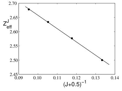
Figure 11: Plot of $Z^{J}_{\rm eff}$ vs $(J+{\scriptstyle\frac{1}{2}})^{-1}$ for the synthetic data as discussed in the text. The line shows the fit to eq. (16) while the $\bullet$ give the synthetic data points with the $\Delta Z^{J}_{\rm eff}\sim(J+{\scriptstyle\frac{1}{2}})^{-2.6}$ dependence.

The $p_{Z}$ exponent derived from the recent GL calculation Gribakin and Ludlow (2004) is depicted in Figure 1. Although GL assume $p_{Z}=2$ when making the extrapolation, the actual exponent extracted from their sequence of $Z_{\rm eff}$ values is $p=2.233$ at $J=10$. The present basis 2 calculation gives $p_{Z}=1.885$ at $J=10$. It is obvious that the GL calculation overestimates the rate at which $\Delta Z^{J}_{\rm eff}$ increments are decreasing. This implies that the GL estimates of $\Delta Z^{J}_{\rm eff}$ will be too small at higher $J$ and this is the case. GL get $\Delta Z^{10}_{\rm eff}=0.0501$ while the CI-Kohn calculation gives $\Delta Z^{10}_{\rm eff}=0.0604$. Consequently, the GL calculation gives $\Delta Z^{J>10}_{\rm eff}=0.48$, while the basis 2 CI-Kohn calculation gives $\Delta Z^{J>10}_{\rm eff}\approx 0.62$. The assertion by GL that their calculation has converged to the region in which the $\Delta Z^{J}_{\rm eff}=B(J+{\scriptstyle\frac{1}{2}})^{-2}$ formula is valid is incorrect.

Besides directly leading to less reliable extrapolation corrections, a related problem with the GL procedure is that it does not have the sensitivity to flag potential problems with the radial basis. A plot of $p_{Z}$ versus $J$ that crosses the $p_{Z}=2$ line is a good indicator of some inadequacy in the basis. There is no indication that GL were aware that their $\Delta Z^{J}_{\rm eff}$ were decreasing much too quickly as $J$ increased, their statement that The use of a $B$-spline basis means that fast convergence is achieved with respect to the number of states with a particular angular momentum is difficult to reconcile with the present analysis. However, it should be noted that do indicate that they could improve the quality of their answers by “pushing harder” the numerics.

The tendency for the GL calculation to overestimate the convergence of the annihilation rate increments probably does not arise from MBPT per se, rather it most likely comes from the underlying single electron basis. Besides the inherently slower convergence at higher $J$ mentioned earlier, another possibility is due to the confinement of the basis to a box of radius 15 $a_{0}$. Confining the basis in this way will result in mean excitation energies (e.g. for predicting the multi-pole polarizabilities) that will eventually increase as $\sim\ell^{2}$, where $\ell$ is the orbital angular momentum, while for a real H atom the mean excitation energy for any $\ell$ is less than 1.0 Hartree Dalgarno and Lewis (1956). Thus the occupancy of the higher $J$ orbitals, which contribute significantly to $Z_{\rm eff}$ will be inhibited, and successive $\Delta Z^{J}_{\rm eff}$ will decrease too rapidly with increasing $J$.

The relevance of these issues is best illustrated by a comparison with the exact value of $Z_{\rm eff}$ which will be taken to be 3.407 at $k=0.4\ a_{0}^{-1}$. This is 0.295 larger than the GL value of 3.112. The underestimation of the higher partial wave contribution in the GL calculation, estimated at $0.14=0.62-0.48$ is responsible for about 50$\%$ of the existing discrepancy.

The discrepancies of GL with the best calculations are are not that severe for $s$-wave scattering since imposition of the $p=2$ condition for $J\geq 10$ prevents the inherent deficiencies in their $B$-spline basis from becoming too excessive. Also $s$-wave $e^{+}$-H scattering system is certainly one of the easier positron annihilation calculations. However, the inadequacy of the GL methodology manifests itself more severely in other positron annihilation situations.

The CI expansion converges quicker for electron-positron annihilations that take place at small distances from the nucleus than for annihilations that take place at large distances Mitroy et al. (2002); Bromley and Mitroy (2002d); Novikov et al. (2004). The presence of the centrifugal barrier for $L>0$ scattering leads to the electron-positron annihilations occurring further from the nucleus. Consequently the convergence problem is more serious for $p$-wave and $d$-wave scattering since a proportionally larger part of $Z_{\rm eff}$ comes from the $J\to\infty$ correction Bromley and Mitroy (2003); Novikov et al. (2004). We have not repeated the earlier $p$-wave calculations Bromley and Mitroy (2003) with a larger radial basis, but a comparison with the CI-Kohn data at $k=0.4\ a_{0}^{-1}$ indicates that the GL calculation again underestimates the impact of the high $J$ orbitals. The CI-Kohn calculation reported in Bromley and Mitroy (2003) gave $\Delta Z^{10}_{\rm eff}=0.0480$ while the GL calculation gave 0.0416. In addition, the CI-Kohn calculation gave $p=1.852$ for $J=10$ while the GL calculation gave $p=2.152$ (it is likely that an infinite basis CI-Kohn calculation would have $p<1.80$ at $J=10$). The GL calculation (which gave $Z_{rmeff}=1.607$) underestimates the $L=1$ $Z_{\rm eff}$ by about 0.18 at $k=0.4$ $a_{0}^{-1}$ (the $T$-matrix calculation gives 1.786 Mitroy and Ratnavelu (1995); Ryzhikh and Mitroy (2000) while van Reeth et.al. gave 1.794 Van Reeth and Humberston (1997, 1998); Gribakin and Ludlow (2004)). It is likely that at least 0.10 of the discrepancy will arise from orbitals with $J\geq 10$.

One of the major results of the GL calculations was their demonstration that the enhancement factor is independent of energy. The enhancement factor can be defined as the factor that the annihilation rate, calculated as a simple product of the electron and positron densities needs to be increased in order to agree with the exact annihilation rate Puska and Nieminen (1994); Mitroy and Ivanov (2002); Novikov et al. (2004). They (GL) based this conclusion solely on a forensic analysis of the $Z_{\rm eff}$ annihilation rate matrix element. Figure 13 of GL reveals that the variation of the $d$-wave enhancement factor with energy is noticeably larger than either the $s$-wave or $p$-wave enhancement factor Gribakin and Ludlow (2004). Since a larger fraction of the $d$-wave $Z_{\rm eff}$ comes from $J\geq 10$, the possibility exists that this stronger energy dependence is due to extrapolation issues as opposed to dynamical effects. Although GL seem unaware of the result, the slow variation of the enhancement factor with energy had been demonstrated in a model potential analysis Mitroy and Ivanov (2002). Comparisons of model potential calculations with ab-initio variational and polarized orbital calculations had shown that a model potential calculation tuned to reproduce the energy dependence of the phase shifts also gave the energy dependence of $Z_{\rm eff}$ Mitroy and Ivanov (2002). The variation of the $d$-wave enhancement factor was determined by tuning a model potential to the large basis phase shifts of Mitroy (1995) and then normalizing to a similar calculation of $Z_{\rm eff}$ Ryzhikh and Mitroy (2000). The variation in the $d$-wave enhancement factor over the energy range from $k=0$ to 0.5 $a_{0}^{-1}$ was less than 4$\%$. Although the model potential result is not conclusive, it does appear that the variation in the $d$-wave $Z_{\rm eff}$ is less than that indicated by the GL calculation.

Another area where application of the GL methodology could lead to larger than anticipated errors is in the determination the angular correlation or the $\gamma$ energy spectrum Dunlop and Gribakin (2006). These two properties depend on the relative momentum of the annihilating electron-positron pair Charlton (1985); Ryzhikh and Mitroy (1999). It is known from investigations of momentum space wave functions that the low momentum part of the wave function largely arise from the large $r$ part of the wave function while the high momentum properties come from the small $r$ part of the wave function McCarthy and Weigold (1991). Under such circumstances, application of the GL method could easily result in errors to the $J\to\infty$ corrections that depend systematically on the $\gamma$-energy or recoil momentum.

VI Summary and Conclusions

Single center methods represent a superficially attractive method to study mixed electron positron systems since existing computer codes can be adapted without too much effort. The penalty associated with this approach is the slow convergence of the binding energy and, more noticeably, the annihilation rate with respect to the partial wave expansion of the single particle basis. The results presented here are generally consistent with the asymptotic limits derived from second-order perturbation theory by Gribakin and Ludlow Gribakin and Ludlow (2002). The actual calculations at finite $J$ generally give increments to the energy (phase shift) and annihilation rate that decrease slightly slower than the GL limits, but the overall trends are compatible with the GL limits.

The tendency for the convergence with respect to the radial basis size to slow down as $J$ increases does have implications for the design of any CI type calculation. Some sort of extrapolation in $J$ is necessary in order to determine the energy and more particularly the annihilation rate. But there is no point in making $J$ bigger if this is done at the expense of the radial basis set. One simply ends up with increments to the energy or annihilation rate which are systematically too small at higher $J$. This problem does not seem to be restricted to the LTO basis used in the present work. Convergence problems at high $J$ are also present for the Gribakin and Ludlow calculations which used a $B$-spline basis Gribakin and Ludlow (2004) and the Saito calculations which used a natural orbital basis Saito (2003a, 2005); Mitroy and Bromley (2005). It is amusing to note that the one of the first manifestations of this problem occurred over 40 years ago Tycko et al. (1958); Schwartz (1962a).

The best methods for estimating the $J\to\infty$ corrections depends on the quality of the underlying calculation. For a low precision calculation, Method I would seem to be appropriate. A low precision calculation can probably be regarded as one with $p_{E}$ or $p_{\Gamma}$ exceeding 4 or 2 respectively when the $J\to\infty$ correction is evaluated (assuming that $p$ approaches its limiting value from below). Methods II or III would seem to be the preferred options for a high precision calculation. As a general principle, inclusion of the second term in the asymptotic series leads to improved $\langle X\rangle^{\infty}$ predictions when compared with asymptotic series with the single term series. Method III is more susceptible to imperfections in the radial basis and should not be applied to the calculation of the annihilation rate unless a very large radial basis set is employed. Irrespective of how the $J\to\infty$ corrections are evaluated, it is essential that the exponents $p$ relating the changes in the expectation values be examined as a test of the quality of the radial basis.

The overall situation regarding the use of single center methods to compute positron-atom phase shifts or energies is that calculation to the sub 1$\%$ accuracy level is achievable for those systems that have a parent atom ionization potential greater than 0.250 Hartree. The $O((J+{\scriptstyle\frac{1}{2}})^{-4})$ convergence means a $J$ of 10 or slightly larger will generally suffice as long as the method used to perform the $J\to\infty$ correction is more sophisticated than those used previously. However, the situation with respect to the annihilation rate is much grimmer and it is not possible to guarantee 1$\%$ accuracy for even the simple $e^{+}$-H system. Here the $O((J+{\scriptstyle\frac{1}{2}})^{-2})$ convergence means the $J\to\infty$ correction is larger, and moreover the slow convergence with respect to the radial basis is further complicated by the fact that it is slower at high $J$ than low $J$. In this case, it appears that “God is on the side of the big basis set” bon .