Roughness and Finite Size Effect in the NYSE Stock-Price Fluctuations

Abstract

We consider the roughness properties of NYSE (New York Stock Exchange) stock-price fluctuations. The statistical properties of the data are relatively homogeneous within the same day but the large jumps between different days prevent the extension of the analysis to large times. This leads to intrinsic finite size effects which alter the apparent Hurst (H) exponent. We show, by analytical methods, that finite size effects always lead to an enhancement of H. We then consider the effect of fat tails on the analysis of the roughness and show that the finite size effects are strongly enhanced by the fat tails. The non stationarity of the stock price dynamics also enhances the finite size effects which, in principle, can become important even in the asymptotic regime. We then compute the Hurst exponent for a set of stocks of the NYSE and argue that the interpretation of the value of H is highly ambiguous in view of the above results. Finally we propose an alternative determination of the roughness in terms of the fluctuations from moving averages with variable characteristic times. This permits to eliminate most of the previous problems and to characterize the roughness in useful way. In particular this approach corresponds to the automatic elimination of trends at any scale.

1 Introduction

The dynamics and fluctuations of stock-prices is represented, at the simplest level, by a random walk which guarantees for the basic property of an efficient market. In the past years it has become clear that one faces a rather subtle and complex form of random walk. Simple correlations of price change are indeed zero at the shortest time but many other features, often related to power law behavior have been discovered (bib1, ). Among the most preeminent one may mention the power law distributions of returns (“fat tails”) and the volatility clustering (bib2, ; bib3, ). These properties, however, are far from exhaustive and other approaches have been introduced in the attempt of describing the subtle correlations of stock-price dynamics.

One of these methods is the attempt to characterize the “roughness” of the dynamics which can provide additional information with respect to the fat tails and volatility. The scaling properties of the roughness can be defined via the so called Hurst exponent $H$ (bib3, ). We consider the roughness problem for high frequency NYSE stock-prices. This means that we take into account all the transactions which occur (tick by tick).

First we discuss the statistical properties of the data set and show that finite size effects are unavoidable and very important. Then we show that fat tails and correlations affect the value of the Hurst exponent in an important way. Finally we analyze the real stock-price fluctuations and argue that the Hurst exponent alone cannot properly characterize their roughness. To this purpose we use a new method to study the roughness which is able to automatically eliminate the trend problem. This is based on the deviation from a suitable moving average and it resolves various ambiguities of the Hurst approach.

The paper is organized in the following way:

In Section 2 we discuss the database for the high frequency samples. This will lead to a crucial role of finite size effects because the data are relatively homogeneous within the same day but there is a large gap in price between the closing of one day and the opening of the next day.

In Section 3 we discuss the general problem associated to the determination of the roughness via the Hurst exponent in view of the anisotropic scaling.

In Section 4 we consider the finite size effects on the roughness exponent in random walks with an analytical approach and then include also the possible effects of fat tails and correlations with Monte Carlo simulations.

In Section 5 we present the roughness analysis for s selection of NYSE stock-prices also as a function of time.

In Section 6 we critically analyze the scaling assumption in relation to the roughness and consider new tools to this purpose which eliminate the trends at all scales automatically.

In Section 7 we discuss the results and present the conclusions.

2 Database properties

We consider as database the price time series of all the transactions of a selection of 20 NYSE stocks. These have been selected to be representative and with intermediate volatility. This corresponds to volumes of $10^{5}-10^{6}$ stocks exchanged per day. We consider 80 days from October 2004 to February 2005.

Figure 1: Behavior of the density of transactions within a day. This concave behavior with a maximum fluctuation up to a factor of two is a general feature for all stocks.

The time series we consider are by a sequential order tick by tick. This is not identical to the price value as a function of physical time but we have tested that the results are rather insensitive to this choice.

The number of transactions per day ranges from 500 to 5000 implying a typical time interval between transactions of a few seconds. The density of operations within a day is characterized by a concave shape which is rather universal as shown in Fig. 1. This means that, with respect to the physical time there are systematic density fluctuations up to a factor of two with a minimum around the center. This effect is obviously eliminated in our tick by tick time, in which physical time is not considered and we have tested that it is not relevant for the roughness properties.

A problem which is very important and rarely discussed in the literature, is the fact that the closing price of a given day is usually very different than the opening price of the next day. A typical behavior is illustrated in Fig. 2. and it shows that these jumps are serious problem in linking the data of one day to those of the next day.

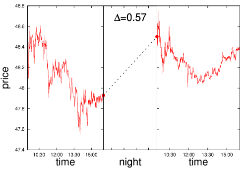
Figure 2: Night jumps between two days. This gap is very large, typically of the order of the total daily fluctuation (see Tab.1). This poses a serious problem in the analysis of roughness because data are reasonably homogeneous only within a single day. This leads to the importance of finite size effects in the analysis.

This means that the data are reasonably homogeneous from the time scale of a few seconds to a few hours but going to longer times can be rather arbitrary due to these large night jumps.

Table 1: Properties of the night jumps with respect to the daily fluctuations of various stocks. The data refer to the average values over 80 trading days. $<|p_{0}-p_{c}|>$: average absolute value of the gap between opening and closing price for each day. $<|\Delta|>$: average of the absolute value of the night jumps. $\sigma_{\Delta}$: variance of the absolute value of the night jumps. $\sigma_{p}$: total daily variance of the price value. $\sigma_{\delta p}$: variance of the price fluctuations between two transactions.

stock	$<|p_{o}-p_{c}|>$	$<|\Delta|>$	$\sigma_{\Delta}$	$\sigma_{p}$	$\sigma_{\delta p}$
AH	0.73494	0.36950	0.59100	0.28539	0.02152
AVO	0.47561	0.18862	0.56508	0.23161	0.01698
BA	0.41926	0.21437	0.42131	0.19530	0.01056
BRO	0.40877	0.15750	0.37375	0.19091	0.01607
CAI	0.81284	0.39238	0.86836	0.31750	0.02323
DRI	0.30753	0.09850	0.23245	0.11490	0.01065
GE	0.22691	0.11688	0.17154	0.10304	0.00652
GLK	0.28272	0.10212	0.23420	0.12998	0.01054
GM	0.35593	0.15725	0.25058	0.14597	0.00833
JWN	0.44531	0.23325	0.45625	0.20444	0.01249
KSS	0.57759	0.29628	0.48844	0.22275	0.01355
MCD	0.24457	0.13850	0.20268	0.10288	0.00758
MHS	0.43605	0.20437	0.40161	0.17267	0.01126
MIK	0.34531	0.62375	3.12751	0.14479	0.01320
MLS	0.55309	0.17287	0.27860	0.21948	0.02045
PG	0.40321	0.24462	0.46493	0.17056	0.00906
TXI	0.79704	0.22362	0.62309	0.33799	0.02964
UDI	0.44679	0.22375	0.80100	0.19003	0.01469
VNO	0.65864	0.21950	0.36921	0.26285	0.02443
WGR	0.40877	0.16937	0.36687	0.17846	0.01681

In Tab. 1 we present a detailed analysis of this phenomenon. For each stock we have in the first column the average over 80 days of the absolute value of the gap between opening and closing price, $(<|p_{o}-p_{c}|>)$, indicated in US $. In the second column we indicate with $<|\Delta|>$ the average of the absolute values of the night jumps. One can see immediately that they are of the same order of magnitude. In the third column $\sigma_{\Delta}$ indicates the variance of the night jumps. These values are really very large and clearly show that there is a strong discontinuity from the closing price to the next day opening. In the fourth column we show the variance of price fluctuation within one day averaged over the 80 days (average single day volatility). Finally in the fifth column we show the variance of the price fluctuations between two transactions. One can see therefore that the night jumps are more than one order of magnitude larger than the typical price change between two transactions. This leads to a very serious problem if one tries to extend these time series beyond the time scale of a single day. In fact, if one simply continues to the next day, one has anomalous jumps for the night which cannot be treated as a standard price change. An alternative possibility could be to artificially eliminate the night jumps and rescale the price correspondingly. This would produce a homogeneous data set which, however, does not correspond to the original data.

This discussion clarifies that there is a fundamental problem in extending the data beyond a single day. Since the transactions within each day range from 500 to 3000, this leads to an important problem of finite size effects in relation to the roughness exponent. In the next section we are going to discuss these finite size effects and show tat they are strongly amplified by the fat tail phenomenon.

3 Roughness and Hurst exponent

Figure 3: Examples of the day price dynamics of two stocks whose behavior, with respect to the roughness, appears very different on a visual inspection. The two stocks have a very similar variance ($\sigma$) for the price distribution. Surprisingly, also the Hurst exponent will be similar for the two cases.

The importance of a characterization of the roughness properties is clearly illustrated in Fig. 3. Here we see the behavior of the price of two stocks which are clearly very different with respect to their roughness properties. The visual difference in roughness, however, does not influence the day volatility $\sigma$, which is almost identical. The idea is therefore to add new concepts to characterize their different behavior. We are going to see in the end that even the Hurst exponent is not really optimal to this purpose and the challenge of this new characterization should proceed along novel lines which we outline at the end of the paper.

We first consider the problem of the characterization of the roughness in the Hurst exponent including the finite size effects. The roughness exponent characterizes the scaling of the price fluctuation as a function of the size of the interval considered.

Originally this exponent was introduced for the time series of the levels of the floods of the Nile river. The basic idea was to construct a profile from these series and analyze its roughness. This implied some peculiar construction which we can avoid because we have the profile directly.

The characterization of the roughness is complicated by the fact that it corresponds to a problem of anisotropic scaling  (bib9, ) and it can lead to confusing results in its practical applications (bib10, ). An example of these difficulties is illustrated by the fact that for the growth of a rough profile the Renormalization Group procedure has to be implemented in a rather sophisticated and unusual way (bib11, ). An illustration of this problem is also given by the fact that the value of the fractal dimension of a rough surface is crucially dependent on the type of procedure one considers (bib11, ). The usual approach is to take the limit of small length scales for which the relation between the dimension of the profile, $D$, and the Hurst exponent is (bib9, ):

$$D=2-H\;\;.$$ (1)

However, if one consider the limit of large scales (not rigorous mathematically but often used in physics), one can get $D=1$ for the Brownian profiles which does not correspond any more to Eq. (1).

In the data analysis one is forced to consider a finite interval and necessarily the two tendencies get mixed. Even considering Eq. (1) one can have various ambiguities. In fact a large Hurst exponent corresponds to small value of the fractal dimension which may appear strange.

Various problems contribute to this possible confusion. The first is how one looks at a scaling law for an anisotropic problem. The scaling for roughness links the vertical fluctuation $\Delta h$ as a function of the interval considered:

$$\Delta h(\Delta L)\sim{\Delta L}^{H}$$ (2)

In a physical perspective one has typically a lower cutoff and looks at the behavior for large values of $\Delta L$. Since for a random walk (Brownian profile) one has $H=1/2$ one could say that if $H>1/2$ this corresponds to a case which is more rough than the Brownian profile. However this is in apparent contradiction with Eq. (1) because the value of $D$, if $H>1/2$, results smaller than the Brownian value $(D=3/2)$. This is because Eq. (1) is derived in the limit $\Delta L\rightarrow 0$ in the spirit of the coverage approach to derive the fractal dimension.

A similar confusion can be given by the existence of trends in the dynamics of the system. Consider for example a straight line behavior for which $\Delta h\sim\Delta L$. In this case one would have $H=1$ and $D=1$, namely the system is not rough in the $\Delta L\rightarrow 0$ perspective but it is very rough in the $\Delta L\rightarrow\infty$ view. In such a situation one should realize that a trend is present and that the system is smooth. However, this distinction is not possible with the Hurst approach.

Actually in the real data one has an upper and a lower limit for $\Delta L$, due to the intrinsic statistical limitation of the sample. The exponent $H$ is then obtained by a fit in a certain range of scales and all the above problems are difficult to sort out.

4 Roughness in a finite size Random Walk

In this section we discuss the role of finite size effects in the determination of the Hurst exponent. We start by deriving some analytical results for a finite size random walk. Consider the function:

$$\!\!\!\!{\mathcal{R}}(n)=\langle\max_{k=(ln+1),(ln+n)}(x_{k})\,-\min_{k=(ln+1),(ln+n)}(x_{k})\rangle_{l}$$ (3)

where $l=1,2,...,\frac{N}{n}$ and $\{x_{1},x_{2},...,x_{N}\}$ are $N$ record in time of a variable $X$. The function ${\mathcal{R}}(n)$ describes the expectation value of the difference between maximum and minimum over an interval of size $n$. ${\mathcal{R}}(n)$, for many records in time is very well described by the following empirical relation:

$$\mathcal{R}(n)\propto n^{H}$$ (4)

where $H$ is the Hurst exponent. Now we want to check which is the effect of the finite size in estimating the Hurst exponent. To perform this analysis we consider a random walk and try to make an analytical calculation of the function $R(n)$.

Suppose that $\{\delta x_{1},\delta x_{2},...\}$ are independent random variables, each taking the value 1 with probability $p$ and -1 otherwise. Consider the sums :

$$x_{n}=\sum_{i=1}^{n}\delta x_{i}$$ (5)

then the sequence $x=\{x_{i}:i\geq 0\}$ is a simple random walk starting at the origin. Now we want to compute the expectation value of the maximum and the minimum of the walk after $n$ steps. In order to do that consider the Spitzer’s identity which relates $\mathbb{E}({M_{n}})$ to $\mathbb{E}\,({x_{n}^{+}})$ in the following way bib12 :

$$\log\Big{(}\sum_{n=0}^{\infty}\,t^{n}\,\mathbb{E}(s^{M_{n}})\Big{)}=\sum_{n=1}^{\infty}\frac{1}{n}\,t^{n}\,\mathbb{E}\,(s^{x_{n}^{+}})$$ (6)

where $M_{n}=\max\,\{x_{i}:0\geq i\geq n\}$ is the maximum of the walk up to time $n$, $x_{n}^{+}=\max\,\{0,x_{n}\}$, $s$ and $t$ are two auxiliary variables which absolute values are smaller than one and $\mathbb{E}$ is the expectation value. Considering the exponential of the Spitzer’s identity and performing the n-nth derivative we obtain:

$$\mathbb{E}\,(s^{M_{n}}) = \frac{1}{n}\sum_{k=1}^{n}\frac{\mathbb{E}(s^{x_{n}^{+}})}{(n-k)!}\,f^{(n-k)}{\big{|}}_{0}\;\;\;\;\;\mbox{where}$$

$$f(t) = \exp(g(t))$$ (7)

$$g(t) = \sum_{n=1}^{\infty}\frac{1}{n}\,t^{n}\,\mathbb{E}\,(s^{x_{n}^{+}})$$

and $f^{(n)}{\big{|}}_{0}$ is the $n$-nth derivative of $f(t)$ calculated in $t=0$. For the derivative one can write a recursive expression:

$$f^{(n)}{\big{|}}_{0}=\sum_{k=1}^{n}\frac{(n-1)!}{(n-k)!}\mathbb{E}\,(s^{x_{k}^{+}})f^{(n-k)}{\big{|}}_{0}$$ (8)

The relation between $\mathbb{E}(M_{n})$ and $\mathbb{E}(s^{M_{n}})$ for a symmetrical probability density function can be obtained by a straightforward calculation bib12a .

$$\mathbb{E}(s^{x_{n}^{+}})=1+\frac{1}{2}\,\mathbb{E}(|x_{n}|)\,\ln(s)+{\mathcal{O}}{(\ln(s))}^{2}$$

By substituting this expression in that of $\mathbb{E}(s^{M_{n}})$ and taking the limit for $s\rightarrow 1$:

$$\mathbb{E}(M_{n})=\lim_{s\rightarrow 1}\frac{\mathbb{E}(s^{M_{n}})-1}{\ln(s)}$$ (9)

The basic final relation is therefore bib12a

$$\mathbb{E}(M_{n})=\sum_{i=1}^{n}\frac{\mathbb{E}(|x_{i}|)}{2i}$$ (10)

From this expression it is possible to derive explicitly the expected value of the maximum as a function of the number of steps of the walk. By considering that a similar expression holds also for the minimum, one can directly compute the effective Hurst exponent for random walk of any size. The specific example of Gaussian increments or $\pm 1$ increments are considered in detail in Ref. bib12a . Replacing the results obtained for $\mathbb{E}(M_{n})$ in the expression of ${\mathcal{R}}(n)$ we can plot the average span as a function of $n$ and execute a fit to estimate the value of $H$. Executing a fit in the region $[10,1000]$ we obtain a value of the slope that is grater then the asymptotic one. In Fig. 4 we shows the result for the effective Hurst exponent that we have obtained performing the fit in the region $[10,n]$ for the random walk with two identical steps $(\pm 1)$. One can see that finite size effects are very important and a seriously affect the apparent value of $H$.

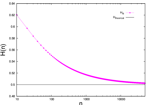
Figure 4: This plot shows the trend obtained fitting the curve ${\mathcal{R}}(n)$ for different values of the size $n$. The results shows a systematic overestimate of Hurst exponent for small size, due to finite size effects. This is a general result and it shows that finite size effects always enhance the apparent Hurst exponent. This enhancement can be understood by considering that, in some sense, a single step would correspond to $H=1$, so the asymptotic value $H=1/2$ is approached from above.

The random walk models considered until now have a distribution of individual steps corresponding to a Gaussian distribution or to two identical steps. Real price differences however, are characterized by a distribution of sizes which strongly deviates from these (“fat tails“). For example, if we consider the histogram of the quantity:

$$S(t)=\ln P(t+1)-\ln P(t),$$ (11)

we find a distributions with large tails, as shown in Fig. 5.

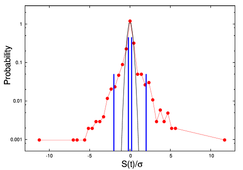
Figure 5: Probability function for high frequency price difference of the BRO stock during a day. The solid line is the Gaussian fit of the data. The boxes represent a model to estimate the effect of the tails for the random walk. The probability is estimate by an histogram given by a value $\pm\epsilon$ which has $0.45$ of probability an a tail $\pm 10\epsilon$ with probability $0.05$. In this plot $\epsilon=0.2$.

To analyze the effect of the fat tails in the evaluation of the Hurst exponent, we can consider a model of random walk with increments that take the values $\delta x=\pm\epsilon$ with probability $0.45$ and $\delta x=\pm 10\epsilon$ with probability $0.05$. The histogram in Fig. 5 represent such a model. We have performed a numerical analysis of the Hurst exponent for a random walk with fat tails to study their role on the finite size effects. To this purpose we have generated $1000$ random walks of this kind of size $n$ with $n=[100:5000]$ and we have calculated the function $R(n)$ for each sample. After calculating the average of $R(n)$, we have considered the plot $R(n)$ as a function of $n$ and the evaluation of $H(n)$ has been performed in the region $[\frac{n}{100};\frac{n}{10}]$. Figure 6 shows the result obtained, a comparison with a normal and a correlated random walk is also shown.

The fact that fat tails and correlations enhance the finite size effects is easy to understand. In case of correlated random walks the effective number of independent steps is strongly reduced. In the case of fat tails instead only the tails give the main contribution to the profile.

This findings could also have implications for very long times if combined with the non stationarity of the price dynamics. It should be considered the possibility that even the asymptotic regime is still altered by these effects. This could suggest a different interpretation of the deviation of $H$ from the value $1/2$, which is usually proposed in terms of long range correlations bib8 .

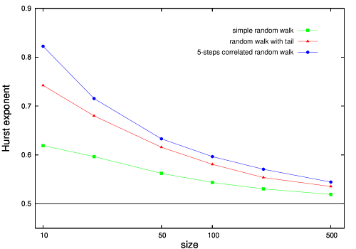
Figure 6: The value of $H(n)$ is shown for three different random walk models: normal, correlated and with fat tails. Finite size effect already present in the normal random walk are amplified by the presence of fat tails and correlations. In the x-axis is plotted the effective size, that is $\frac{n}{10}$. The values are averaged over $1000$ realizations.

The Fig. 6 shows the inefficiency of the Hurst exponent’s approach to the study of the roughness for systems with a small size. The results are clearly affected by the effect of a finite size and the interpretation of $H>1/2$ as a long range correlation could be misleading.

5 Analysis of NYSE stocks

First we consider the Hurst analysis for the two stocks plotted in Fig. 3 and the relative results are shown in Fig. 7.

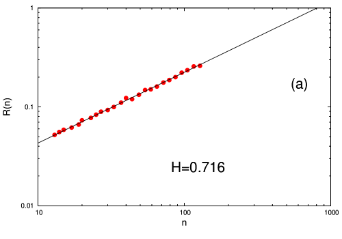
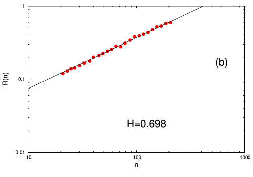
Figure 7: Analysis in terms of the Hurst exponent of the two stocks shown in Fig. 3. The case (a) refers to the stock which appears smooth, while (b) is the other one. One can see that the value of $H$ is very similar despite the apparent differences between the two behavior (Fig. 3).

The values of the two exponents $H$ are very similar in spite of the large difference of the two stocks in their apparent roughness properties. This shows that the exponent $H$ is not suitable to characterize the different roughness properties of the two stocks.

Table 2: Hurst exponent for 20 NYSE stocks. $H$ is the average daily value over the 80 days. $H_{max}$ and $H_{min}$ are the maximum and the minimum and $\sigma$ the variance. $<N>$ is the average number of transactions per day.

stock	$H$	$H_{max}$	$H_{min}$	$\sigma$	$<N>$
AH	0.599	0.732	0.489	0.0215	1535.77
AVO	0.615	0.785	0.501	0.0170	1296.71
BA	0.573	0.694	0.478	0.0106	3323.37
BRO	0.662	0.792	0.557	0.0161	853.91
CAI	0.641	0.751	0.478	0.0232	1052.58
DRI	0.575	0.699	0.445	0.0106	1446.65
GE	0.526	0.653	0.406	0.0065	5598.83
GLK	0.627	0.780	0.484	0.0105	1114.01
GM	0.574	0.677	0.462	0.0083	3405.84
JWN	0.579	0.738	0.457	0.0125	2025.67
KSS	0.570	0.686	0.438	0.0135	2789.09
MCD	0.559	0.691	0.417	0.0076	3480.63
MHS	0.612	0.750	0.460	0.0113	1792.51
MIK	0.591	0.752	0.456	0.0132	1377.84
MLS	0.635	0.914	0.496	0.0204	759.27
PG	0.551	0.662	0.456	0.0091	4135.80
TXI	0.636	0.776	0.473	0.0296	733.68
UDI	0.679	0.781	0.524	0.0147	774.25
VNO	0.622	0.777	0.506	0.0244	883.78

We then consider the entire series of $20$ stocks and the results are reported in Tab. 2. Here $H$ represents the a daily value averaged over 80 days. Then $H_{max}$ and $H_{min}$ are the maximum and the minimum values respectively, $\sigma$ is the variance averaged over the 80 values and $<N>$ is the average number of transactions per day. In Fig. 8 we report the time behavior of $H(t)$ for the 80 days for the two stocks of Fig. 3. With respect to previous analysis of the time dependence of H(t) bib7 , we can observe that the daily variability of single stocks is much larger than that of global indices over long times. In addition also the average is appreciably larger.

A general result is that the value of $H$ is systematically larger than $1/2$. The usual interpretation would be to conclude that long range correlations are present bib8 . However, in view of our previous discussion we would instead propose that this deviation from $1/2$ is precisely due to finite size effects, combined with the fat tail phenomenon. A further support to this interpretation is that if we built a long time series by eliminating the night jumps, one observes a convergency towards the value $1/2$. Also one may note that stocks with a relatively large number of transactions per day ($<N>$), like for example GE stock, are much closer to the random walk value $H=1/2$.

The fact that apparently different profiles with respect to the roughness lead to value of $H$ which are very similar is due to a variety of reasons. The overall enhancement with respect to the standard value $1/2$ is, in our opinion, mostly due to the finite size effects phenomenon. However, this does not explain why two profiles which appear very different, like those in Fig. 3, finally, lead to very similar values of $H$. This is probably due to the fact that the Hurst approach tends to mix the role of trends with fluctuations and in the next section we are going to propose a different method to resolve this problem.

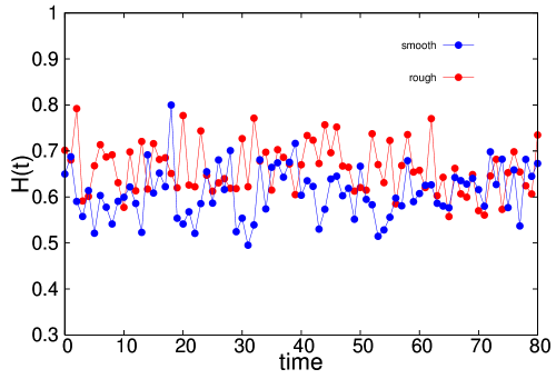
Figure 8: Time dependence of the Hurst exponent $H(t)$ for the two stocks shown in Fig. 3.

To complete our analysis, we consider the generalized Hurst exponent in the spirit of Ref. bib14 . To this purpose we analyze a q-th order price difference correlation function defined by:

$$G_{q}(\tau)=<|p(x)-p(x+\tau)|^{q}>^{\frac{1}{q}}$$ (12)

The generalized Hurst exponent $H_{q}$ can be defined from the scaling behavior of $G_{q}(\tau)$:

$$G_{q}(\tau)\sim{\tau}^{H_{q}}$$ (13)

For a simple random walk $H_{q}=H=1/2$ independently of $q$. We have calculate the function $G_{q}(\tau)$ for the two test-stocks.

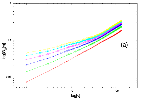
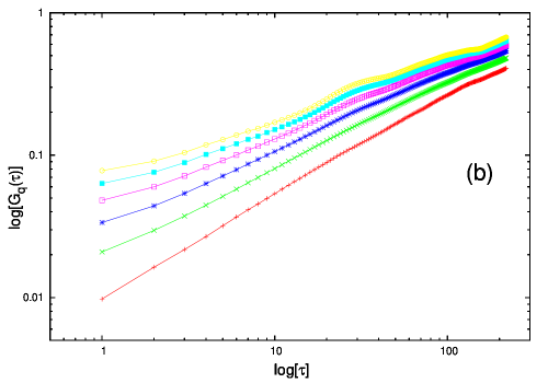
Figure 9: $G_{q}(\tau)$ as a function of $\tau$ in a log-log scale for the two test-stock ((a) is the smooth and (b) the rough one). In both (a) and (b), from bottom to top $q=1,2,3,4,5,6$.

The results are shown in Fig. 9 and show that $H_{q}$ is not a constant but strongly depends on $q$. This result provides an evidence that the characteristics of the profile are dominated by the large jumps due to the fat tail properties.

6 New approach to roughness as fluctuation from Moving Average

In this section we consider a new method to characterize the roughness. The basic idea is to be able to perform an automatic detrendization of the price signal. This can be achieved by the difference between the price variable and its moving average defined in an optimal way. At each transaction point $t_{i}$ we define the moving average of the price $P(t_{i})$, with a characteristic time $\tau$, as:

$$P_{\tau}(t_{i})=\frac{1}{N_{\tau}}\sum_{j}P(t_{j})$$ (14)

where $N_{\tau}$ are the number of transactions in the time interval $[-\tau/2:\tau/2]$. This function corresponds to the symmetric average over an interval of size $N_{\tau}$ around $t_{i}$.

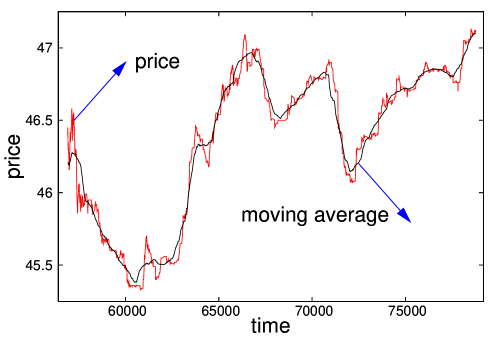
Figure 10: Example of price fluctuations and the corresponding moving average. In our case we consider a symmetrized moving average defined as the average of the price over a symmetric interval of total size $\tau$.

One can then consider the maximum deviation of $P(T_{i})$ from $P_{\tau}(t_{i})$ over an interval of a certain size, in our case we consider a single day:

$$R_{\tau}=\max_{i}|P(t_{i})-P_{\tau}(t_{i})|$$ (15)

This may appear similar to the standard definition of roughness which gives the absolute fluctuation in a time interval $\tau$. Instead the use of $R_{\tau}$ corresponds to an automatic detrendization which appears more appropriate to study the roughness. Our approach is similar to the one of Ref. bib13 , but with the difference that we use a symmetrized definition of the moving average while Ref. bib13 defines the moving average only with respect to a previous time interval.

In Fig. 11 we show the values of $R_{\tau}$ for the two stocks shown in Fig. 3 and, for comparison, the same stocks analyzed with the Hurst method. One can see that the fluctuations from the moving average are more appropriate to describe the difference between these stocks which cannot be detected with the standard Hurst approach.

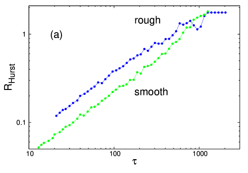
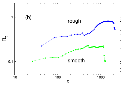
Figure 11: (a) Fluctuations over intervals of different size ($\tau$) defined by the differences between maximum and minimum values over intervals of size $\tau$. These curves were used in the previous sections to compute the Hurst exponent in the standard way. The two curves refer to the two stock of Fig. 3. One can observe that the slope is similar for the two cases and, at relatively large scale ($\tau$) even the amplitudes become rather similar. (b) In this case the amplitudes are defined by the fluctuations from the moving averages as given by Eq. (15). In this case there is a marked difference in slope and even more in amplitude. This example clarifies that this new definition of roughness can be more useful to classify the stock dynamics.

7 Discussion and Conclusions

We have considered the roughness properties as a new element to characterize the high frequency stock-price fluctuations. The data considered include all transactions and show a large night jump between one day and the next. For this reasons the dataset are statistically homogeneous only within each day. This leads to a serious problem of finite size effects which we have analyzed by using various random walk models as examples. We have computed the effective Hurst exponent as a function of the size of the system. The basic result is that the finite size effects lead to a systematic enhancement of the effective Hurst exponent and this tendency is amplified by the inclusion of fat tails and eventual correlations.

An analysis of real stock-price behavior leads to the conclusion that most of the deviations from the random walk value ($H=1/2$) are indeed due to finite size effects. Considering the importance of non-stationarity phenomenon one may conjecture that the finite size effects could be important even for long series of data.

Concerning the roughness analysis we conclude that the standard Hurst approach is not very sensitive in order to characterize the various stock-price behaviors. We propose a different roughness analysis based on the fluctuations from a symmetrized moving average. This has the advantage of an automatic detrendization of the signal without any ad hoc modification of the original data. This new method appears much more useful than the standard one in order to characterize the fluctuations behavior of different stock as shown clearly by the analysis of the two cases in Fig. 3.

References

- (1) B. Mandelbrot, Fractals and Scaling in Finance (Springer Verlag, New York, 1997).
- (2) R.N. Mantegna, H.E. Stanley, An Introduction to Econophysics (CambridgeUniversity Press, Cambridge, 2000).
- (3) J.P. Bouchaud, Theory of Financial Risk, (Cambridge University Press, Cambridge, 2000).
- (4) H.E. Hurst, Transaction of the American Society of Civil Engineers 116, 770-808 (1951).
- (5) S.O. Cajueiro, B. Tabak, Physica A 336, 521-537 (2004).
- (6) D. Grech, Z. Mazur, Physica A 336, 133-145 (2004).
- (7) A. Carbone, G. Castelli, H.E. Stanley, Physica A 344, 267-271 (2004).
- (8) T. Di Matteo, T. Aste, M.M. Dacorogna, Journal of Banking and Finance 29, 827-851 (2005).
- (9) A.L. Barabasi, H.E. Stanley, Fractal Concepts in Surface Growth (Cambridge University Press, Cambridge, 1994).
- (10) L. Pietronero, Order and Chaos in Nonlinear Physical System, edited by S. Lundqvist, N. H. March, and M. Tosi (Plenum Publishing Corporation, New York, 1988), 227.
- (11) C. Castellano, M. Marsili, L. Pietronero, Phys. Rev. Lett. 80, 3527 (1998).
- (12) G. Grimmet, D. Stirzaker, Probability and Random Processes, (Oxford University Press, Oxford, 2001).
- (13) V. Alfi, F. Coccetti, M. Marotta, A. Petri, L. Pietronero, Physica A, in print 2006, cond-mat/0601230.
- (14) J. Asikainen, S. Majaniemi, M. Dubé, T. Ala-Nissila, Phys. Rev E 65, 052104 (2002).
- (15) E. Alessio, A. Carbone, G. Castelli, V. Frappietro, Eur. Phys. J. B 27, 197-200 (2002).