Networking Effects on Cooperation in Evolutionary Snowdrift Game

Abstract

The effects of networking on the extent of cooperation emerging in a competitive setting are studied. The evolutionary snowdrift game, which represents a realistic alternative to the well-known Prisoner’s Dilemma, is studied in the Watts-Strogatz network that spans the regular, small-world, and random networks through random re-wiring. Over a wide range of payoffs, a re-wired network is found to suppress cooperation when compared with a well-mixed or fully connected system. Two extinction payoffs, that characterize the emergence of a homogeneous steady state, are identified. It is found that, unlike in the Prisoner’s Dilemma, the standard deviation of the degree distribution is the dominant property in a re-wired network that governs the extinction payoffs.

I Introduction

Evolutionary game theory has become an important tool for investigating and understanding cooperative or altruistic behavior in systems consisting of competitive entities. These systems may occur in a wide range of problems in different disciplines and include physical, biological, ecological, social, and political systems. Mathematicians, biologists, and physicists alike have found the phenomena of emergence of cooperative behavior fascinating. Since the ground-breaking work on repeated or iterated games based on the Prisoner’s Dilemma (PD) game by Axelrod axelrod ; axelrod1 , there has been a continuous effort on exploring the determining factors on possible cooperative behavior in evolutionary games based on the PD game and its variations trivers ; nowak ; nowak1 ; hauert ; nowak2 ; lieberman , with a recent emphasis on the effects of spatial structures such as regular lattices nowak1 ; hauert ; nowak3 ; doebeli ; killingback and networks lieberman ; abramson ; kim ; ebel ; masuda ; wu ; santos . Remarkably, it was found that cooperation can be induced in a repeated PD game by cleverly designed strategies. Spatial structures, e.g., lattices or networks, are found to favor cooperative behavior in the evolutionary PD game. The two subjects involved in networked games, i.e., emergence phenomenon and the physics of networks albert , are among the most rapidly growing branches in physics.

The present work was motivated by the recent concerns on whether the PD game should be the sole model for studying emerging cooperative phenomena hauert . Due to practical difficulties in accurately quantifying the payoffs in game theory, the snowdrift game (SG) has been proposed as possible alternative to the PD game. Previous work on the SG have focused on the effects of connectivity in structures such as lattices hauert and fully connected networks hauert ; hofbauer . The latter is also referred to as the well-mixed case in the literature. Here, we investigate the networking effects on an evolutionary snowdrift game hauert ; sugden ; smith within the Watts-Strogatz (WS) watts ; albert model of small world constructed by randomly re-wiring a regular network. Starting with a random mixture of competing nodes of opposite characters, we found that (i) the steady-state population may consist of only one kind of nodes or a mixture of nodes of different characters, depending on degree $K$ in a regular lattice before re-wiring and the extent of re-wiring $q$; (ii) for a wide range of payoffs, a re-wired network suppresses the fraction of cooperative nodes in the steady state and hence the overall level of cooperation, when compared with a fully connected network or well-mixed case; (iii) networking effect on the critical payoffs for the extinction of one kind of nodes in the steady state depends sensitively on the width or standard deviation of the degree distribution induced by re-wiring.

The plan of the paper is as follows. The evolutionary snowdrift game and the Watts-Strogatz network structure are introduced in Sec. II. Section III gives the numerical results in regular lattices. Two extinction payoffs are identified. An analytic expression for the extinction payoff of defective character is given, together with a discussion on the discrepancy between observed value and theoretical value of the extinction payoff for runs with finite time steps. Section IV gives the numerical results in re-wired networks. The dependence on the re-wiring probability is found to be governed by the standard deviation of the degree distribution of the re-wired network. In Sec. V, we give an approximate expression for the extinction payoff and summarize our results.

II Model

The basic snowdrift game, which is equivalent to the hawk-dove or chicken game sugden ; smith , is most conveniently described using the following scenario. Consider two drivers hurrying home in opposite directions on a road blocked by a snowdrift. Each driver has two possible actions – to shovel the snowdrift (cooperate (C)) or not to do anything (not-to-cooperate or “defect” (D)). This is similar to the PD game in which each player has two options: to cooperate or to defect. If the two drivers cooperate, they could be back home on time and each will get a reward of $b$. Shovelling is a laborious job with a total cost of $c$. Thus, each driver gets a net reward of $R=b-c/2$. If both drivers take action D, they both get stuck, and each gets a reward of $P=0$. If only one driver takes action C and shovels the snowdrift, then both drivers can get through. The driver taking action D (not to shovel) gets home without doing anything and hence gets a payoff $T=b$, while the driver taking action C gets a “sucker” payoff of $S=b-c$. The SG is, therefore, given by the following payoff matrix:

$$\begin{array}[]{ccc}&\begin{array}[]{cc}C&D\end{array}\\ \begin{array}[]{c}C\\ D\end{array}&\left(\begin{array}[]{cc}R&S\\ T&P\end{array}\right).\end{array}$$ (1)

The matrix element gives the payoff to a player using a strategy listed in the left hand column when the opponent uses a strategy in the top row. The SG refers to the case $b>c>0$, leading to $T>R>S>P$. This ordering of the payoffs defines the SG. Without loss of generality, it is useful to assign $R=1$ so that the payoffs can be characterized by a single parameter $r=c/2=c/(2b-c)$ for the cost-to-reward ratio. In terms of $0<r<1$, we have $T=1+r$, $R=1$, $S=1-r$, and $P=0$. For a player, the best action is: to take D if the opponent takes C, otherwise take C. A larger value of $r$ tends to encourage the action D. The SG becomes the PD when the cost $c$ is high such that $2b>c>b>0$, which amounts to the ranking $T>R>P>S$ neumann ; rapoport . Therefore, the SG and PD game differ only by the ordering of $P$ and $S$. Due to the difficulty in measuring payoffs in game theory, the SD has been proposed to be a possible alternative to the PD game in studying emerging cooperative phenomena hauert ; hofbauer .

Evolutionary snowdrift game amounts to letting the character of a connected population of inhomogeneous players evolve, according to their performance hauert . Consider $N$ players represented by the nodes of a network. Initially, the nodes are randomly assigned to be either of C or D character. The character of each node is updated every time step simultaneously, according to the following procedure. At each time step, every node $i$ interacts with all its connected $k_{i}$ neighbors and gets a payoff per neighbor $\overline{V}_{i}=V_{i}/k_{i}$, where $V_{i}$ is obtained by summing up the $k_{i}$ payoffs after comparing characters with its neighbors. Here, $k_{i}$ is the degree of node $i$. Every node $i$ then randomly selects a neighbor $j$ for possible updating or evolution. To compare the performance of the two nodes $i$ and $j$, we construct

$$w_{ij}=(\overline{V_{j}}-\overline{V_{i}})/(T-P)=(\overline{V_{j}}-\overline{V_{i}})/(1+r).$$ (2)

If $w_{ij}>0$, then the character of node $i$ is replaced by the character of node $j$ with probability $w_{ij}$, and thus node $i$ becomes the offspring of node $j$. The denominator $(1+r)$ in $w_{ij}$ is, therefore, included as a normalization factor. If $w_{ij}<0$, then the character of node $i$ remains unchanged. In the long time limit, a state will be attained with possible coexistence of nodes of both characters. The fraction of $C$-nodes $f_{C}$, which is often called the frequency of cooperators hauert , measures the extent of cooperation in the whole system and is determined by the structure of the underlying network and the payoff parameter $r$. In a fully connected network, $f_{C}=1-r$ hauert ; hofbauer . In two-dimensional lattices with nearest-neighboring and next-nearest neighboring connections, it has recently been observed that the spatial structure tends to lower $f_{C}$ hauert , when compared with a fully connected network. In contrast, spatial connections are found to enhance $f_{C}$ in evolutionary PD games. We note that one may define $w_{ij}$ in different ways. Popular alternatives of $w_{ij}$ in evolutionary games include the use of the total payoff instead of an average payoff per neighbor for which the effects of a spread in the degrees of different nodes will be much more prominent and allowing for the possibility of replacing the character of a node by that of a neighboring node with lower payoff. In our choice of $w_{ij}$, a node will only have a chance to be replaced if it encounters a better performing node.

The physics of complex networks albert is a fascinating research area of current interest. Here, the nodes in an evolutionary SG are connected in the form of the Watts-Strogatz watts small-world model. Starting with a one-dimensional regular world consisting of a circular chain, i.e., periodic boundary condition, of $N$ nodes with each node having a degree $2K$ connecting to its $2K$ nearest neighbors, each of the $K$ links to the right hand side of a node is cut and re-wired to a randomly chosen node with a probability $q$. This simple model gives the small world effect watts , which refers to the commonly observed phenomena of small separations between two randomly chosen nodes in many real-life networks albert , for $q\sim 0.1$. The parameter $q$ ($0\leq q\ \leq 1$) thus takes the network from a regular world through the small world to a random world, with a fixed mean degree $\langle k\rangle=2K$. Here, we aim at understanding how the frequency of cooperators $f_{C}$ behaves as the parameters characterizing the the spatial structure $K$ and $q$ change, and as the payoff parameter $r$ characterizing the evolutionary dynamics changes.

III Results: Regular world

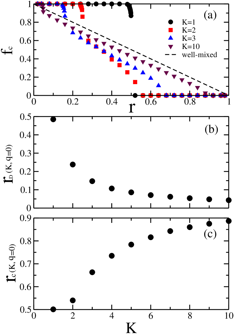
Figure 1: (Color online) (a) The frequency of cooperators $f_{C}$ as a function of the payoff parameter $r$ in a one-dimensional Watts-Strogatz network of size $N=10^{3}$ nodes with $K=1$, $2$, $3$, $10$ before re-wiring ($q=0$). The run time is $10^{4}$ time steps. The dashed line indicates the result $f_{C}=1-r$ for a fully connected network. (b) The extinction payoff $r_{D}(K,q=0)$ as a function of $K$. (c) The extinction payoff $r_{C}(K,q=0)$ as a function of $K$.

Figure 1(a) shows $f_{C}$ as a function of $r$ in regular lattices ($q=0$) of $N=10^{3}$ nodes with different values of $K$. The dashed line gives the result $f_{C}=1-r$ for the well-mixed case. The key features are: (i) there exists a value $r_{D}(K,q=0)$ so that $f_{C}=1$ for $r<r_{D}$, i.e., the extinction of D-nodes and all nodes become cooperative in nature, (ii) for $r<r_{D}$, $f_{C}$ is enhanced when compared with the well-mixed case, (iii) for a wide range of $r$, the frequency of cooperators drops below that in the well-mixed case, (iv) there exists a value $r_{C}(K,q=0)$ so that $f_{C}=0$ for $r>r_{C}$, i.e., the extinction of cooperative nodes remark . These extinction payoffs thus characterize a transition between a homogeneous and an inhomogeneous population as the payoff $r$ is varied. Figures 1(b) and 1(c) show that the extinction payoff for defectors (cooperators) $r_{D}$ ($r_{C}$) decreases (increases) monotonically with $K$ in regular lattices. Numerically, it is found that for $K=1,2$, $r_{D}(K,q=0)$ is close to $1/2K$; while for $K\geq 3$, $r_{D}(K,q=0)$ is closer to $1/(2K+1)$. In addition, we observe that for $K\geq 3$, the relation $2r_{D}+r_{C}\approx 1$ is satisfied. The feature (iii) is analogous to that observed in two-dimensional lattices hauert . We have also found that $r_{D}$ and $r_{C}$ are independent of the number of nodes $N$, as long as $N\gg 1$. As the shortest path $L=N/4K$ scales with $N$ in regular lattices, the results imply that the $K$-dependence of the extinction payoffs does not come from $L$, although $L$ is an important quantity in the description of networks. Clearly, the time it takes the system from the initial configuration to that in the long time limit would depend on $N$ and hence $L$.

Analytically, the value of $r_{D}(K,q=0)$ can be estimated as follows. Recall that a higher value of $r$ promotes D-character and $r_{D}$ refers to the highest value of $r$ below which no D-node exists. Since replacements are carried out probabilistically, it is, therefore, important to consider cases where there are only a few D-nodes and how these patterns will be replaced. Note that for any value of $K$, a single D-node in an otherwise C-node environment will not be replaced. The reason is the following. The average payoff for the single D-node is $\overline{V_{D}}=1+r$. Note that only the C-nodes that are connected to the D-node may be involved in a possible evolution. For these C-nodes, their average payoff $\overline{V_{C(1D)}}=1-r/2K$, where the subscript indicate that it is the average payoff for a C-node that is linked to one D-node. Thus, for the whole range of $r$, $\overline{V_{D}}>V_{C(1D)}$ and thus a single D-node will not be replaced by its connected C-neighbors.

This leads us to consider the patterns involving D-nodes, called the last surviving patterns, that can be replaced by C-nodes in one time step. The case of $K=1$ serves to illustrate the key ideas in estimating $r_{D}$. For $K=1$, the single D-node pattern will be evolved into one with a pair of neighboring D-nodes. The chain becomes that of …CCCCDDCCCC…. Because each D-node has a D-neighbor and the D-D payoff is $P=0$, the average payoff of the D-nodes becomes $\overline{V_{D}}=(1+r)/2$. The payoff of the C-nodes that are linked to a D-node is $\overline{V_{C(1D)}}=1-r/2$. By equating $\overline{V_{D}}$ and $\overline{V_{C(1D)}}$, we obtain an estimate of $r_{D}=1/2$ for $K=1$, which agrees with numerical results. For $r<1/2$, $\overline{V_{C(1D)}}>\overline{V_{D}}$ and thus the D-D dimer pattern may evolve into an all-C chain, provided that both D-nodes randomly pick the neighboring C-node and evolve into C-character with the probability $w_{ij}$ in the same time step. Thus, the key features for a last surviving pattern are: (i) we need at least two connected D-nodes, and (ii) the C-nodes that are connected to only one of these surviving D-nodes have a higher chance to replace the D-nodes. The discussion also serves to point out the importance of run time in numerical studies. When the system evolves to the last surviving pattern, the pattern may or may not evolve into an all-C pattern. It only happens probabilistically. The time it takes, even when $r<r_{D}$, for the all-C pattern to emerge depends on the values of $r$ and $K$. For $r\rightarrow r_{D}$ and for larger values of $K$, the time may be exceedingly long so that a smaller value of $r_{D}$ than that theoretically allowed will be determined numerically.

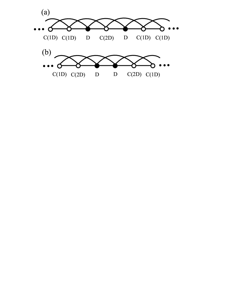
Figure 2: Two last surviving patterns in $K=2$ regular lattices for estimating the extinction payoff $r_{D}$. Typically, these patterns consist of two connected D-nodes in a background of C-nodes. The C-nodes connected to one D-node (labelled C(1D)) and connected to two D-nodes (labelled C(2D)) have different average payoffs. $r_{D}$ is found by equating the average payoffs $\overline{V_{C(1D)}}$ and $\overline{V_{D}}$.

Extending the argument to $K=2$ regular lattices, a single D-node will evolve into one of the last surviving patterns shown in Figure 2. In both patterns, there are two types of neighboring C-nodes. For the C-nodes connected to only one D-node, the average payoff $\overline{V_{C(1D)}}=1-r/4$. For the C-nodes connected to two D-nodes, $\overline{V_{C(2D)}}=1-r/2$. For the D-nodes, $\overline{V_{D}}=3(1+r)/4$. Note that in general $\overline{V_{C(1D)}}>\overline{V_{C(2D)}}$. Since there are more C-nodes with one D-neighbor in the pattern in Figure 2(a) than Figure 2(b), the D-nodes in Figure 2(a) are most likely to be the last surviving pattern in numerical simulations. There are two values of $r$ that are of interest. For $r<1/5=1/(2K+1)$, we have $\overline{V_{C(1D)}}>\overline{V_{C(2D)}}>\overline{V_{D}}$. Therefore, all the neighboring C-nodes have a finite probability to replace the two D-nodes in one time step. This is why it is easier to observe an all-C pattern for $r<1/5$. In principle, $r_{D}$ can be found by equating $\overline{V_{C(1D)}}$ and $\overline{V_{D}}$, giving $r_{D}=1/4$. However, for $1/5<r<1/4$, we have $\overline{V_{C(1D)}}>\overline{V_{D}}>\overline{V_{C(2D)}}$. These inequalities imply that even if we arrive at the patterns in Figure 2, the chance of replacing both D-nodes by C-character is small, since only the C-nodes connected to one D-node can carry out the replacement. Instead, the D-nodes may replace the C-nodes linked to both D-nodes to arrive at a pattern with more D-nodes. This prevents the all-C pattern from emerging in any run of reasonably long run time. This effect is obviously more severe as $K$ increases, as there will be more C-nodes with two D-neighbors.

Generalizing the argument to arbitrary value of $K$, we have $\overline{V_{D}}=(1+r)(1-1/2K)$ and $\overline{V_{C(1D)}}=1-r/2K$. Thus, in principle, $r_{D}(K,q=0)=1/2K$. However, for any practical run times, the all-C pattern is hard to observe for $1/(2K+1)<r<1/(2K)$, except for $K=1$ and $2$. Thus, the numerical results in Figure 1, which are obtained by fixing the run time to be $t=10^{4}$ time steps, give $r_{D}\approx 1/(2K+1)$ for $K\geq 3$. We have tried longer run times, e.g., $3\times 10^{5}$ time steps, and the value of $r_{D}$ only tends to approach the value $1/2K$ very slowly.

IV Results: Watts-Strogatz re-wired networks

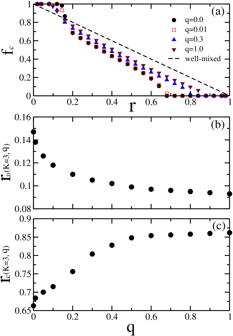
Figure 3: (Color online) (a) The frequency of cooperators $f_{C}$ as a function of the the payoff parameter $r$ in Watts-Strogatz networks of $K=3$ for different values of the re-wiring probability $q=0$, $0.01$, $0.3$, $1.0$. The dashed line indicates the result $f_{C}=1-r$ for a fully connected network. (b) The extinction payoff $r_{D}(K,q)$ as a function of $q$ for $K=3$. (c) The extinction payoff $r_{C}(K,q)$ as a function of $q$ for $K=3$.

Going beyond regular lattices, Figure 3(a) shows $f_{C}$ as a function of $r$ in Watts-Strogatz (WS) networks with different re-wiring probabilities $q=0.01$, $0.3$ and $1.0$. The network consists of $N=10^{3}$ nodes and $K=3$, with the run time fixed at $t=10^{4}$ time steps. Results in a regular lattice ($q=0$) and fully connected networks (dashed line) are also included for comparison. It is noted that the effect of increasing $q$ for fixed $K$ is similar to increasing $K$ for fixed $q=0$ (regular lattices). The main features are that as $q$ increases, the extinction payoff $r_{D}$ decreases and the $f_{C}$ is higher than that in a regular lattice with the same value of $K$ for a large range of $r$. Figures 3(b) and (c) show that, for fixed $K=3$, the extinction payoff $r_{D}$ ($r_{C}$) drops (rises) with the re-wiring probability $q$. We have checked that while the shortest path $L(q)$ changes sensitively with $q$, it is however not the determining factor for the extinction payoffs. Will the clustering coefficient $C$ matter? For regular lattices, $C$ increases with $K$ and saturates at large $K$ following $C(0)=3(2K-2)/[4(2K-1)]$ watts ; albert . If the drop in $r_{D}$ with $K$ in regular lattices were attributed to the increase in $C$, then one would have expected $r_{D}$ to increase with $q$ as $C(q)\simeq C(0)(1-q)^{3}$ decreases with $q$ in WS networks watts ; albert . This is, however, not what is observed in numerical results. Therefore, the clustering coefficient $C$ is also not a determining factor for $r_{D}$ and $r_{C}$. These observations are in sharp contrast to the networking effects in evolutionary PD games abramson ; kim ; ebel ; masuda ; wu . Noting that the WS networks have a fixed $\langle k\rangle=2K$ with or without re-wiring, $r_{D}$ and $r_{C}$ cannot be determined by the mean degree $\langle k\rangle$. Thus, $r_{D}$ and $r_{C}$ are not determined by the commonly studied quantities in networks.

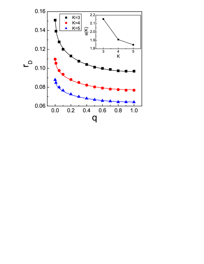
Figure 4: (Color online) The extinction payoff $r_{D}(K,q)$ is plotted against $q$ for different values of $K=3$, $4$, $5$. The results are obtained by runs of $3\times 10^{5}$ time steps. The lines are obtained by fitting to a form given by Eq.(4). The inset gives the dependence of the fitting parameter $a(K)$ on $K$.

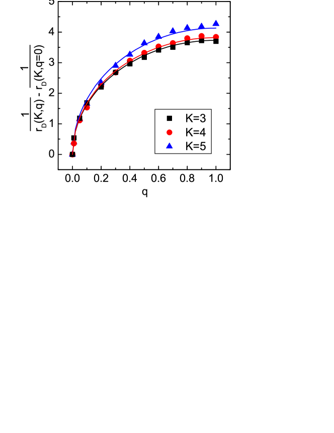
Figure 5: (Color online) By suitably choosing the quantity on the y-axis, the set of scattered data in Fig. 4 can be shown to follow a similar functional dependence on $q$. The dependence is found to follow that of $\sqrt{2q-q^{2}}$ in the standard deviation of the degree distribution in Watts-Strogatz networks after re-wiring for fixed $K$. The lines are obtained by using the fitting parameters obtained in Fig. 4.

The results in Figures 1 and 3 revealed that the extinction payoffs $r_{D}(K,q)$ and $r_{C}(K,q)$ depend on both the structural parameters $K$ and $q$. It does remain an intriguing problem of which geometrical property (properties) of a re-wired network determines $r_{D}$ and $r_{C}$ in the Watts-Strogatz networks. In what follows, we will focus on analyzing $r_{D}(K,q)$, as $r_{C}\approx 1-2r_{D}$. Figure 4 shows collectively the numerical results (symbols) of $r_{D}(K,q)$ for different values of $K$ and $q$, for a longer fixed run time of $3\times 10^{5}$ time steps. As discussed, the numerical results for $r_{D}(K,q=0)$ in a regular lattice may not come out to be $1/2K$ even using a longer run time, we could avoid this problem and focus on the effects of re-wiring, i.e., $q\neq 0$, by exploring the behavior of the difference in $r_{D}(K,q)$ and $r_{D}(K,0)$. Interestingly, we found that by plotting $(1/r_{D}(K,q)-1/r_{D}(K,q=0))$ as a function of $q$, the numerical data for different values of $K$ basically follow the same functional form, as shown by the symbols in Figure 5. Examining the $q$-dependence, we notice that the behavior is similar to that in the standard deviation $\sigma(K,q)$ of the degree distribution $P(k)$ in the Watts-Strogatz networks. The re-wiring process changes $P(k)$ gradually from a delta-function at $k=2K$ for $q=0$ to a distribution that has a lower cutoff at $k=K$ with a finite $\sigma(K,q)$ that increases with $q$ albert . More specifically,

$$\sigma(K,q)=\sqrt{K}\cdot\sqrt{2q-q^{2}},$$ (3)

which follows from the degree distribution of the Watts-Strogatz model. Motivated by this observation, we use the numerical data in Figure 4 and perform a fit to the functional form

$$r_{D}(K,q)=\frac{1}{\frac{1}{r_{D}(K,0)}+a(K)\sigma(K,q)},$$ (4)

where $a(K)$ is a fitting parameter. The first term in the denominator of Eq. (4) imposes the restriction that the fitted line must pass through the $q=0$ data point. The fitted lines are also shown in Figure 4. With only one fitting parameter for each value of $K$, the lines fit the data accurately. This implies that the $q$-dependence follows that in $\sigma(K,q)$. The fitting parameters are found to be $a(3)=2.154$, $a(4)=1.910$, and $a(5)=1.847$. Note that $a(K)$ drops with $K$ (see inset in Fig. 4). Since $\sigma(K,q)$ carries a factor of $\sqrt{K}$, the combination $b(K)=a(K)\sqrt{K}$ becomes quite insensitive to $K$, with $b$ increasing from $3.73$ for $K=3$ to $4.13$ for $K=5$. As a consistency check, we also plot the fitted lines in Figure 5, using the same coefficients $a(K)$ as obtained in Figure 4. Note that even for $q=1$, the spread in the data and fitted lines is small, reflecting the weak $K$-dependence in the coefficients $b(K)$. The extinction payoff is thus found to be described by

$$\frac{1}{r_{D}(K,q)}=\frac{1}{r_{D}(K,q=0)}+b(K)\;\sqrt{2q-q^{2}},$$ (5)

where $b$ carries only a weak $K$-dependence. Our results on the extinction payoff $r_{D}(K,q)$ in the Watts-Strogatz networks can be summarized as follows. The dependence on $K$ is dominated by that in $r_{D}(K,q=0)$ and the $q$-dependence follows that of the standard deviation $\sigma(K,q)$ of the degree distribution.

V Discussion

Our analytic approach in getting $r_{D}$ in regular lattices (see Sec. III) can also be applied to re-wired networks. The difference is that in a re-wired network, different nodes may have different number of neighbors, i.e., different degrees. Again, we consider a last surviving pattern with two connected D-nodes with otherwise C-neighbors. Let $k_{D}$ be the degree of one of the D-nodes. Therefore, this D-node has $(k_{D}-1)$ C-neighbors and one D-neighbor. Let $k_{C}$ be the degree of one of these C-neighbors or the typical degree of these C-neighbors. We assume that the C-nodes are only connected to one D-node, as they are the ones more likely to replace the D-nodes. For the D-node, the average payoff is:

$$\overline{V_{D}}=\frac{k_{D}-1}{k_{D}}+\frac{(k_{D}-1)r}{k_{D}},$$ (6)

while for the C-node, the average payoff is:

$$\overline{V_{C}}=1-\frac{r}{k_{C}}.$$ (7)

For regular lattices, $k_{C}=k_{D}=2K$ and $r_{D}=1/2K$ is recovered when we equate $\overline{V_{D}}$ to $\overline{V_{C}}$. In addition, as $K$ increases in a regular lattice, $r_{D}\rightarrow 0$, which is the result in the well-mixed case. In general, equating Eq. (6) and Eq. (7) gives

$$r^{\prime}_{D}=\frac{k_{C}}{(k_{D}-1)k_{C}+k_{D}}.$$ (8)

The meaning of $r^{\prime}_{D}$ is that, if a last surviving pattern of the considered structure is approached in a numerical simulation, then for $r<r^{\prime}_{D}$, such a pattern may become all-C in one time step.

Equation (8) suggests several possibilities on estimating $r_{D}$. A lower bound of $r_{D}$ can be constructed by noting that a D-node occupying a node of high degree can take advantage of the many C-neighbors and hence requires a lower value of $r$ to replace it. Similarly, a surrounding C-node with fewer C-neighbors has lower average payoff and hence is harder to replace the D-nodes. Let $k_{max}(K,q)$ be the maximum degree in a re-wired network for given $K$ and $q$. The minimum degree in a Watts-Strogatz network is close to $K$ after re-wiring. An extreme (but rare) case is that of a D-node occupying a degree with $k_{max}$ being surrounded by C-nodes that occupy nodes with degree $K$. A more reasonable assumption is to take the degree of the C-nodes as the mean degree $2K$, as any one of the C-nodes may be picked in the evolution step. We can substitute $k_{D}=k_{max}(K,q)$ and $k_{C}=2K$ to get an estimate of a lower bound

$$r_{D}^{lower}=\frac{2K}{2K(k_{max}(K,q)-1)+k_{max}(K,q)}.$$ (9)

We have checked that Eq. (9) indeed gives values that are lower than numerical results. More interestingly, $k_{max}(K,q)$ turns out to depend on $q$ through the standard deviation $\sigma(K,q)$ remark1 . Hence, Eq. (9) does reproduce the drop of $r_{D}$ as $q$ increases, as observed in Fig.4.

It is also possible to relate Eq. (8) to Eqs. (4) and (5). Assuming that, after averaging over runs in numerical studies, that $k_{C}$ and $k_{D}$ can both be approximated as some typical degree $k_{ave}(K,q)$, then Eq. (8) suggests that the extinction payoff would be

$$r_{D}=\frac{1}{k_{ave}(K,q)}.$$ (10)

Since the dynamics in evolutionary SG depends on the average payoffs, which in turn depends on the geometrical structure of the neighborhood of a node, we expect in general $k_{ave}$ is different from the mean degree $2K$. Instead, D-node tends to survive easily by staying on nodes of higher degree. Comparing Eq.(10) with Eq. (4), we notice that the fitted result to numerical data implies that

$$k_{ave}(K,q)=\frac{1}{r_{D}(K,q=0)}+a(K)\sigma(K,q).$$ (11)

where the first term should in principle be $2K$.

In summary, we investigated the extent of cooperation that would emerge in a networked evolutionary snowdrift game. The random re-wiring model of Watts and Strogatz is used. Comparing to a fully connected network, a spatial structure of regular lattices suppresses $f_{C}$ over a wide range of the payoff $r$ and re-wiring lowers the suppression. We identified two extinction payoffs $r_{D}$ and $r_{C}$. For regular lattices, $r_{D}$ should take on the value of $1/2K$, although a value closer to $1/(2K+1)$ is usually observed in numerical studies. The dependence of $r_{D}(K,q)$ on $K$ and $q$ is highly non-trivial. The key network property that gives the $q$-dependence is found to be the standard deviation of the degree distribution. This finding, in turn, implies that it is the existence of nodes with higher degrees due to randomly re-wiring that plays a dominant role in determining the extinction payoffs.

- (1) R. Axelrod and W.D. Hamilton, Science 211, 1390 (1981).
- (2) R. Axelrod, The Evolution of Cooperation (Basic Books, New York, 1984).
- (3) R. Trivers, Social Evolution (Cummings, Menlo Park, 1985).
- (4) M.A. Nowak and K. Sigmund, Nature (London) 355, 250 (1992).
- (5) M.A Nowak and R.M. May, Nature (London) 359, 826 (1992).
- (6) C. Hauert and M. Doebell, Nature (London) 428, 643 (2004).
- (7) M.A. Nowak, A. Sasaki, C. Taylor, and D. Fudenberg, Nature (London) 428, 646 (2004).
- (8) E. Lieberman, C. Hauert, and M.A. Nowak, Nature (London) 433, 312 (2005).
- (9) M.A. Nowak and R.M. May, Int. J. Bifur. Chaos 3, 35 (1993); M.A. Nowak, S. Bonhoeffer, and R.M. May, Int. J. Bifur. Chaos 4, 33 (1994); M.A. Nowak, S. Bonhoeffer, and R.M. May, Proc. Natl. Acad. Sci. USA 91, 4877 (1994).
- (10) M. Doebeli and N. Knowlton, Proc. Natl. Acad. Sci. USA 95, 8676 (1998).
- (11) T. Killingback, M. Doebeli, and N. Knowlton, Proc. R. Soc. Lond. B 266, 1723 (1999).
- (12) G. Abramson and M. Kuperman, Phys. Rev. E 63, 030901(R) (2001).
- (13) B.J. Kim, A. Trusina, P. Holme, P. Minnhagen, J.S. Chung, and M.Y. Choi, Phys. Rev. E 66, 021907 (2002).
- (14) H. Ebel and S. Bornholdt, Phys. Rev. E 66, 056118 (2002).
- (15) N. Masuda and K. Aihara, Phys. Lett. A 313, 55 (2003).
- (16) Z.X. Wu, X.J. Xu, Y. Chen, and Y.H. Wang, Phys. Rev. E 71, 037103 (2005).
- (17) F.C. Santos and J.M. Pacheco, Phys. Rev. Lett. 95, 098104 (2005).
- (18) R. Albert and A.-L. Barabási, Rev. Mod. Phys. 74, 47 (2002).
- (19) J. Hofbauer and K. Sigmund, Evolutionary Games and Population Dynamics (Cambridge Univ. Press, Cambridge, UK, 1998).
- (20) R. Sugden, The Economics of Rights, Co-operation and Welfare (Blackwell, Oxford, UK, 1986).
- (21) J.M. Smith, Evolution and the Theory of Games (Canbridge University Press, Cambridge, UK, 1982).
- (22) D.J. Watts, S.H. Strogatz, Nature (London) 393, 440 (1998); D.J. Watts, Small Worlds: The Dynamics of Networks Between Order and Randomness (Princeton, New Jersey, 1999).
- (23) J. von Neumann and O. Morgenstem, Theory of Games and Economic Behavior (Princeton University Press, Princeton, NJ, 1953).
- (24) A. Rapoport and A.M. Chammah, Prisoner’s Dilemma (University of Michigan Press, Ann Arbor, 1965).
- (25) This is the case except for a few isolated values of with for which the chain can be evolved into a configuration with a majority of D-nodes with isolated C-nodes distributed at equal distances.
- (26) We have checked that the maximum degree for given and takes on the form , where depends on only weakly and takes on values close to for different values of . As increases with , in Eq. (9) drops with , as observed in numerical results.