Parallel Computing for 4-atomic Molecular Dynamics Calculations

Abstract

We report the results of intensive numerical calculations for four atomic H₂+H₂ energy transfer collision. A parallel computing technique based on LAM/MPI functions is used. In this algorithm, the data is distributed to the processors according to the value of the momentum quantum number $J$ and its projection $M$. Most of the work is local to each processor. The topology of the data communication is a simple star. Timings are given and the scaling of the algorithm is discussed. Two different recently published potential energy surfaces for the H${}_{2}-$H₂ system are applied. New results obtained for the state resolved excitation-deexcitation cross sections and rates valuable for astrophysical applications are presented. Finally, more sophisticated extensions of the parallel code are discussed.

Keywords: Parallel algorithm, LAM/MPI application, Star-type cluster, quantum dynamics.

I Introduction

In modern competitive research in science and technology high performance computing plays a paramount role. Its importance is derived from the fact, that correctly chosen and designed numerical methods and algorithms properly adapted to parallel and multithreaded techniques can essentially reduce computation time and active memory usage [1]. The importance of this fact is especially magnified in calculating quantum molecular dynamics and atomic collisions due to their massive complexity.

Generally speaking, modern computation research in scientific applications has taken two twists. First, to provide efficient and stable numerical calculations, and second to provide for the proper use of various high performance techniques like LAM/MPI, OpenMP and/or others [2]. Now it is equally important not only to get the correct numerical results, but also to design and implement efficient high performance algorithms and get faster results with less memory. We would like to note here, that a program/software, which is designed for specific problems in computational physics, chemistry or biology should be able to perform calculations in either serial or parallel.

The problem we selected for our parallel computation in this work is taken from molecular/chemical physics. Specifically we carry out detailed quantum-mechanical calculations of state-resolved cross sections and rates in hydrogen molecular collisions H₂+H₂. Interaction and collisions between hydrogen molecules, and hydrogen molecular isotopes, for example H₂+HD, is of great theoretical and experimental interest for many years [3-14]. Specifically we will explore the quantum-mechanical 4-atomic system shown in Fig. 1 using six independent variables resulting in the full description of the system. The main goal of this investigation is to carry out a comparative analysis of two recently published potential energy surfaces (PESs) for H${}_{2}-$H₂.

Our motivation for selecting this problem is, that the hydrogen molecule plays an important role in many areas of astrophysics [15-16] This is the simplest and most abundant molecule in the universe especially in giant molecular clouds. Because of low number of electrons in H${}_{2}-$H₂ this is one of few four-center systems for which potential energy surface (PES) can be developed with very high precision. Therefore H₂+H₂ may be also a benchmark collision for testing other dynamical methods. Additionally, the H₂+H₂ elastic and inelastic collisions are of interest in combustion, spacecraft modeling and at the present hydrogen gas is becoming a very important potential energy supplier, see for example [17].

We test two PESs: the first one is a global 6-dimensional potential from work [18], the second one is very accurate interaction potential calculated from the first principles [19]. Because we are going to carry out detailed quantum-mechanical calculations using two PESs the computation work is at least doubled and therefore even more time consuming. We needed to carry out convergence tests with respect to different chemical and numerical parameters for both PESs and, finally, we have to make production calculations for many points of kinetic energy collisions. Clearly, an application of parallel computing techniques shall be very useful in this situation.

In this work we carry out parallel computation with up to 14 processors. The scattering cross sections and their corresponding rate coefficients are calculated using a non reactive quantum-mechanical close-coupling approach. In the next section we will shortly outline the quantum-mechanical method and the parallelization approach. Our calculations for H₂+H₂, scaling and timing results are presented in Sec. III. Conclusions are given in Sec. IV. Atomic units (e=m_e=$\hbar$=1) are used throughout the work.

Figure 1: 4-body coordinates for the H${}_{2}-$H₂ system used in this work.

II Method

II-A Quantum-mechanical approach

In this section we briefly represent a quantum-mechanical approach and the parallel algorithm used in this work. The 4-atomic H${}_{2}-$H₂ system is shown in Fig. 1. It can be described by six independent variables: $r_{1}$ and $r_{2}$ are interatomic distances in each hydrogen molecule, $\Theta_{1}$ and $\Theta_{2}$ are polar angles, $\Phi$ is torsional angle and $R$ is intermolecule distance. The hydrogen molecules are treated as linear rigid rotors, that is distances $r_{1}=r_{2}=0.74A$ are fixed in this model. We provide a numerical solution for the Schrödinger equation for an $ab+cd$ collision in the center of the mass frame, where $ab$ and $cd$ are linear rigid rotors.

To solve the equation the total 4-atomic H${}_{2}+$H₂ wave function is expanded into channel angular momentum functions $\phi^{JM}_{\alpha^{\prime}}(\hat{r}_{1},\hat{r}_{2},\vec{R})$ [4]. This procedure followed by separation of angular momentum provides a set of coupled second order differential equations for the unknown radial functions $U^{JM}_{\alpha}(R)$

$$\left(\frac{d^{2}}{dR^{2}}-\frac{L(L+1)}{R^{2}}+k_{\alpha}^{2}\right)U_{\alpha}^{JM}(R)=2M_{12}\sum_{\alpha^{\prime}}\int<\phi^{JM}_{\alpha}(\hat{r}_{1},\hat{r}_{2},\vec{R})$$

$$|V(\vec{r}_{1},\vec{r}_{2},\vec{R})|\phi^{JM}_{\alpha^{\prime}}(\hat{r}_{1},\hat{r}_{2},\vec{R})>U_{\alpha^{\prime}}^{JM}(R)d\hat{r}_{1}d\hat{r}_{2}d\hat{R},$$ (1)

where $\alpha\equiv(j_{1}j_{2}j_{12}L)$, $j_{1}+j_{2}=j_{12}$, $j_{12}+L=J$ and $j_{1},j_{2},L$ are quantum angular momentum corresponding to vectors $\vec{r}_{1}$, $\vec{r}_{2}$ and $\vec{R}$ respectively, $M_{12}=(m_{a}+m_{b})(m_{c}+m_{d})/(m_{a}+m_{b}+m_{c}+m_{d})$, $V(\vec{r}_{1},\vec{r}_{2},\vec{R})$ is the potential energy surface for the 4-atomic system $abcd$, and $k_{\alpha}$ is channel wavenumber.

Figure 2: Schematic diagram of the topology of interprocessor communication: an example of a star-type cluster with one main and four satellite computers.

We apply the hybrid modified log-derivative-Airy propagator in the general purpose scattering code MOLSCAT [20] to solve the coupled radial equations (1). We have tested other propagator schemes included in the code. Our calculations showed that other propagators are also quite stable for both the H${}_{2}-$H₂ potentials considered in this work.

Since all experimentally observable quantum information about the collision is contained in the asymptotic behaviour of functions $U^{JM}_{\alpha}(R\rightarrow\infty)$, the log-derivative matrix is propagated to large $R$-intermolecular distances. The numerical results are matched to the known asymptotic solution to derive the physical scattering $S$-matrix [4]. The method was used for each partial wave until a converged cross section was obtained. It was verified that results are converged with respect to the number of partial waves as well as the matching radius $R_{max}$ for all channels included in the calculations. Cross sections for rotational excitation and relaxation phenomena can be obtained directly from the $S$-matrix. In particular the cross sections for excitation from $j_{1}j_{2}\rightarrow j^{\prime}_{1}j^{\prime}_{2}$ summed over final $m^{\prime}_{1}m^{\prime}_{2}$ and averaged over initial $m_{1}m_{2}$ are given by

$$\sigma(j^{\prime}_{1},j^{\prime}_{2};j_{1}j_{2},\epsilon)={\pi}/{(2j_{1}+1)(2j_{2}+1)k_{\alpha\alpha^{\prime}}}\sum_{Jj_{12}j^{\prime}_{12}LL^{\prime}}(2J+1)|\delta_{\alpha\alpha^{\prime}}-S^{J}(j^{\prime}_{1},j^{\prime}_{2},j^{\prime}_{12}L^{\prime};j_{1},j_{2},j_{12},L;E)|^{2}.$$ (2)

The kinetic energy is $\epsilon=E-B_{1}j_{1}(j_{1}+1)-B_{2}j_{2}(j_{2}+1),$ where $B_{1(2)}$ are rotation constants of rigid rotors $ab$ and $cd$ respectively.

The relationship between a rate coefficient $k_{j_{1}j_{2}\rightarrow j^{\prime}_{1}j^{\prime}_{2}}(T)$ and the corresponding cross section $\sigma_{j_{1}j_{2}\rightarrow j^{\prime}_{1}j^{\prime}_{2}}(E_{kin})$ can be obtained through the following weighted average

$$k_{j_{1}j_{2}\rightarrow j^{\prime}_{1}j^{\prime}_{2}}(T)=\frac{8k_{B}T}{\pi\mu}\frac{1}{(k_{B}T)^{2}}\int_{\epsilon_{s}}^{\infty}\sigma_{j_{1}j_{2}\rightarrow j^{\prime}_{1}j^{\prime}_{2}}(\epsilon)e^{-\epsilon/k_{B}T}\epsilon d\epsilon,$$ (3)

where $T$ is temperature, $k_{B}$ is Boltzmann constant, $\mu$ is reduced mass of the molecule-molecule system, and $\epsilon_{s}$ is the minimum kinetic energy for the levels $j_{1}$ and $j_{2}$ to become accessible.

II-B Parallelization

In this work to support parallel computation the following machines are used: Sun Netra-X1 (UltraAX-i2) with 128 MB RAM (512 MB Swap) and 500 Mhz UltraSPARC-IIe processor. The master computer is SunFire v440 with 8 GB RAM four 1.062 Ghz UltraSPARC-IIIi processors. The system is schematically shown in Fig. 2. In this work we apply LAM/MPI to provide the parallel environment in the cluster.

It is important in the parallel algorithm used in this work, that calculations for specific values of $J$ and $M$ are essentially independent. In the PMP MOLSCAT program [21], which is used the parallelization is done over the loop on values $J$ and $M$. The code distributes the required $JM$ pairs across the available processors. The computational work distribution is shown schematically in Fig. 3. The same idea has been used in works [22, 23] for semiquantal atomic collisions. In these works the parallelization was done along the impact factor $\rho$ of colliding particles, because the solution of the resulting dynamical equations doesn’t depend on $\rho$. It is well known, that in the semiclassical approach the impact factor $\rho$ is an analog of quantum $J$ number.

Figure 3: $J/M$-parallelization method, see text.

As mentioned above, in the quantum-mechanical approach used in this work, a partial wave expansion is applied. A set of coupled channel differential equations has to be solved for many values of the total angular momentum $J$. To calculate the state resolved cross sections and then the rate coefficients (3) the resulting $S$-matrix elements have to be summed from different $J$s. Calculations for a single $J$ can be broken into two or more sectors corresponding to different values of $M$, which is a projection of $J$.

There are two methods to distribute the work among satellite computers. In the static method in the beginning of the job each computer makes a list of the total $J/M$ tasks to be solved. Then each computer selects a subset of the tasks to carry out. Obviously each computer has to get a different subset and an approach needs to be used which gives an approximately equal amount of work to each computer. There is no interprocessor communication in this method.

In the case of a dynamic approach one computer acts as a dispatcher. It makes a list of all the $J/M$ tasks to be done, then waits for the computational processes to call in requesting work. Starting with the longest tasks, the dispatcher hands out $J/M$ tasks to computing processes until all of them have been completed. The next time the computational process asks for work, the dispatcher sends it a message, and the computational process then does its end-of-run cleanup and exits.

III Results

Our results from the parallel calculations using MPI functions to determine rotational transitions in collisions between $para/para$- and ortho-/ortho-hydrogen molecules:

$$\mbox{H}_{2}(j_{1})+\mbox{H}_{2}(j_{2})\rightarrow\mbox{H}_{2}(j^{\prime}_{1})+\mbox{H}_{2}(j^{\prime}_{2}).$$ (4)

are presented in this section together with scaling results.

As we mentioned in the Introduction we are applying the new PESs from the works [18] and [19]. The DJ PES [19] is constructed for the vibrationally averaged rigid monomer model of the H₂$-$H₂ system to the complete basis set limit using coupled-cluster theory with single, double and triple excitations. A four term spherical harmonics expansion model was chosen to fit the surface. It was demonstrated, that the calculated PES can reproduce the quadrupole moment to within 0.58 % and the experimental well depth to within 1 %.

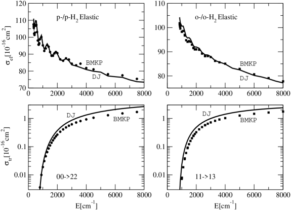
Figure 4: Rotational state resolved integral cross sections for elastic scattering in the case of para-/para- and ortho-/ortho-hydrogen and transitions, when $j_{1}=j_{2}=0\rightarrow j^{\prime}_{1}=2,j^{\prime}_{2}=2$ and $j_{1}=j_{2}=1\rightarrow j^{\prime}_{1}=1,j^{\prime}_{2}=3$. Calculations are done with the BMKP and DJ PESs (the compensating factor of 2 is included only in the elastic cross sections).

The bond length was fixed at 1.449 a.u. or 0.7668 Å. DJ PES is defined by the center-of-mass intermolecular distance, $R$, and three angles: $\theta_{1}$ and $\theta_{2}$ are the plane angles and $\phi_{12}$ is the relative torsional angle. The angular increment for each of the three angles defining the relative orientation of the dimers was chosen to be $30^{\circ}$.

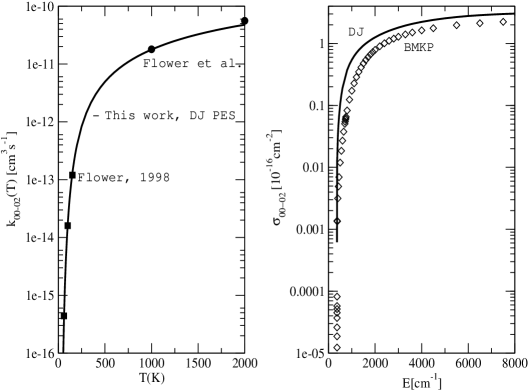
Figure 5: Temperature dependence of the state-resolved thermal rate constant (left panel) and corresponding cross section (right panel) for the transition $j_{1}=j_{2}=0\rightarrow j^{\prime}_{1}=2,j^{\prime}_{2}=0$. Results from other works for the thermal rate $k_{00-02}(T)$ are also included. The results for the DJ PES are given in solid lines. The diamonds are the theoretical data of this work calculated with the BMKP PES.

The BMKP PES [18] is a global six-dimensional potential energy surface for two hydrogen molecules. It was especially constructed to represent the whole interaction region of the chemical reaction dynamics of the four-atomic system and to provide an accurate as possible van der Waals well. In the six-dimensional conformation space of the four atomic system the conical intersection forms a complicated three-dimensional hypersurface. The authors of the work [18] mapped out a large portion of the locus of this conical intersection.

The BMKP PES uses cartesian coordinates to compute distances between four atoms. We have devised some fortran code, which converts spherical coordinates used in Sec. 2 to the corresponding cartesian coordinates and computes the distances between the four atoms. In all our calculations with this potential the bond length was fixed at 1.449 a.u. or 0.7668 Å as in DJ PES.

The main goal of this work is to carry out quantum-mechanical calculations for different transitions in $p$-H₂+$p$-H₂ and $o$-H₂+$o$-H₂ collisions and to provide a comparative study of the two PESs presented above. The energy dependence of the elastic integral cross sections $\sigma_{el}(E_{kin})$ are represented in Fig. 4 (upper plots) together with the state-resolved integral cross sections $\sigma_{j_{1}j_{2}\rightarrow j^{\prime}_{1}j^{\prime}_{2}}(E_{kin})$ for the $j_{1}=j_{2}=0\rightarrow j^{\prime}_{1}=2,j^{\prime}_{2}=2$ and $j_{1}=j_{2}=1\rightarrow j^{\prime}_{1}=1,j^{\prime}_{2}=3$ rotational transitions (lower plots) for both the BMKP and DJ PESs respectively. As can be seen both PESs provide the same type of the behaviour in the cross section. These results are in basic agreement with recent calculations, but using a time-dependent quantum-mechanical approach [10]. Our calculation show, that DJ PES generates higher values for the cross sections.

A large number of test calculations have also been done to secure the convergence of the results with respect to all parameters that enter into the propagation of the Schrödinger equation. This includes the intermolecular distance $R$, the total angular momentum $J$ of the four atomic system, $N_{lvl}$ the number of rotational levels to be included in the close coupling expansion and others (see the MOLSCAT manual [20]).

We reached convergence for the integral cross sections, $\sigma(E_{kin})$, in all considered collisions. In the case of DJ PES the propagation has been done from 2 Å to 10 Å, since this potential is defined only for those specific distances. For the BMKP PES we used $r_{min}=1$ Å to $r_{max}=30$ Å. We also applied a few different propagators included in the MOLSCAT program.

A convergence test with respect to the maximum value of the total orbital momentum showed, that $J_{max}=100$ is good enough for the considered range of energies in this work. We tested various rotational levels $j_{1}j_{2}$ included in the close coupling expansion for the numerical propagation of the resulting coupled equations (1). In these test calculations we used two basis sets: $j_{1}j_{2}$=00, 20, 22, 40, 42 with total basis set size $N_{lvl}=13$ and $j_{1}j_{2}$=00, 20, 22, 40, 42, 44, 60, 62 with $N_{lvl}=28$. We found [24], that the results are quite stable for the 00$\rightarrow$20 and 00$\rightarrow$22 transitions and somewhat stable for the highly excited 00$\rightarrow$40 transition. Nontheless, for our production calculations we used the first basis set.

It is important to point out here, that for comparison purposes we don’t include the compensating factor of 2 mentioned in [5]. However, in Fig. 4 (upper plots) and in our subsequent calculations of the thermal rate coefficients, $k_{jj^{\prime}}(T)$, the factor is included.

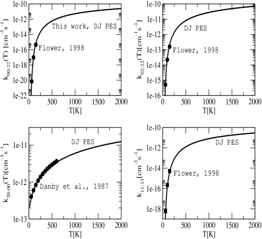
Figure 6: Temperature dependence of the state-resolved thermal rate constants for the $j_{1}=j_{2}=0\rightarrow j^{\prime}_{1}=2,j^{\prime}_{2}=2$, $j_{1}=0,j_{2}=2\rightarrow j^{\prime}_{1}=2,j^{\prime}_{2}=2$, $j_{1}=2,j_{2}=0\rightarrow j^{\prime}_{1}=0,j^{\prime}_{2}=0$ and $j_{1}=1,j_{2}=1\rightarrow j^{\prime}_{1}=1,j^{\prime}_{2}=3$. Results obtained with the DJ PES. Theoretical data from other works are included.

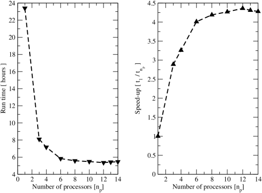
Figure 7: Computation time and speed-up $t_{1}/t_{n_{p}}$ depending on number of parallel processors $n_{p}$ using the dynamic approach, see text.

The differences in the cross sections of the two potentials are reflected in the state-resolved transition states $j_{1}=0,j_{2}=0\rightarrow j^{\prime}_{1}=0,j^{\prime}_{2}=2$, as shown in Fig. 5 (right panel). It seems that the DJ PES can provide much better results, as seen in the same figure in the left panel, when we present the results for the corresponding thermal rates $k_{00-02}(T)$ calculated with the DJ potential together with results of other theoretical calculations. The agreement is perfect. Thus, one can conclude, that DJ PES is better suited for the H${}_{2}-$H₂ system. In Fig. 6 we provide thermal rates for different transition states calculated with only the DJ PES and in comparison with other theoretical data obtained within different dynamical methods and PESs. Again the agreement is very good.

In Fig. 7 we present an example of our timing results using the dynamic method for a specific H${}_{2}(j_{1})$+H${}_{2}(j_{2})$ calculations. It can be seen, that including additional processors reduces the computation time. Here we present two results. The left plot shows dependence of the computing time on amount of active parallel processors. The right plot illustrates the degree of speed-up of the calculations. The speed-up for a fixed test calculation is defined as $t_{1}/t_{n_{p}}$, where $t_{1}$ is the calculation with only one processor and $t_{n_{p}}$ with $n_{p}$ processors.

IV Conclusion

We carried out parallel computations for state-resolved rotational excitation and deexcitation cross sections and rates in molecular $para$-/$para$- and ortho-/ortho-H₂ collisions of astrophysical interest. The LAM/MPI technique allowed us to speed up the computation process at least $\sim 4.5$ times within our 14 processor Sun Unix cluster. We tested the two newest potential energy surfaces for the considered systems. Thus the application of the parallel algorithm reduced the computation time used to test the two potentials. A test of convergence and the results for cross sections and rate coefficients using two different potential energy surfaces for the H${}_{2}-$H₂ system have been obtained for a wide range of kinetic energies.

We would like to point out here, that the hydrogen problem is very important for many reasons. The main motivation has been described in the introduction of this paper. It is also necessary to stress, that the hydrogen-hydrogen collision may be particularly interesting in nanotechnology applications, when the system is confined inside a single wall carbon nanotube (SWNT) [25].

Careful treatment of such collisions can bring useful information about the hydrogen adsorption mechanisms in SWNTs and quantum sieving selectivities [26]. However, in this problem particular attention should be paid not only to the H${}_{2}-$H₂ potential, but also to the many body interaction between H₂ molecules and the carbon nanotube [27-28]. The inclusion of additional complex potentials in the Schrödinger equation may essentially increase the computation difficulties.

It is also very attractive to upgrade the four-dimensional model for the linear rigid rotors used in this work to complete six-dimensional consideration of the H${}_{2}+$H₂ collisions. However, because of two additional integrations over $r_{1}$ and $r_{2}$ distances such calculations should be very time consuming

$$\left(\frac{d^{2}}{dR^{2}}-\frac{L(L+1)}{R^{2}}+k_{\alpha}^{2}\right)U_{\alpha}^{JM}(R)=2M_{12}\sum_{\alpha^{\prime}}\int\int<\phi^{JM}_{\alpha}(\hat{r}_{1},\hat{r}_{2},\vec{R})\chi_{vj_{1}j_{2}}(r_{1},r_{2})$$

$$|V(\vec{r}_{1},\vec{r}_{2},\vec{R})|\chi_{v^{\prime}j^{\prime}_{1}j^{\prime}_{2}}(r_{1},r_{2})\phi^{JM}_{\alpha^{\prime}}(\hat{r}_{1},\hat{r}_{2},\vec{R})>U_{\alpha^{\prime}}^{JM}(R)d^{3}\vec{r}_{1}d^{3}\vec{r}_{2}d\hat{R}.$$ (5)

Here $\chi_{v^{\prime}j^{\prime}_{1}j^{\prime}_{2}}(r_{1},r_{2})$ is the product of the real vibrational wavefunctions of the two molecules

$$\chi_{vj_{1}j_{2}}(r_{1},r_{2})=w_{v_{1}j_{1}}(r_{1})w_{v_{2}j_{2}}(r_{2}),$$ (6)

where $v$ designates the vibrational quantum numbers $v_{1}$ and $v_{2}$ [29]. Nontheless, the application of a parallel computing techniques together with shared memory methodology could be a very effective computational approach, as it was partially demonstrated in this work.

Although our calculations revealed, that both the H${}_{2}-$H₂ PESs used in this work can provide the same type of behaviour in regard to cross sections and rates, there are still significant differences. Considering the results of these calculations we conclude that subsequent work is needed to further improve the H${}_{2}-$H₂ PES, and that work will require parallel processing if it is to be done in a timely manner.

References

- [1] D.M. Medvedev, E.M. Goldfield, S.K. Gray, Comput. Phys. Commun. 166 (2005) 94.
- [2] R. Chandra, R. Menon, L. Dagum, D. Kohr, D. Maydan, J. McDonald, ”Parallel Programming in OpenMP”, Elsevier, Morgan Kaufmann (2000).
- [3] H. Rabitz, J. Chem. Phys., 57, (1972) 1718.
- [4] S. Green, J. Chem. Phys., 62 (1975) 2271; J. Chem. Phys., 67 (1977) 715.
- [5] G. Danby, D.R. Flower, T.S. Monteiro, Mon. Not. R. Astr. Soc., 226 (1987) 739.
- [6] D.W. Schwenke, J. Chem. Phys., 89 (1988) 2076.
- [7] D.R. Flower, Mon. Not. R. Astron. Soc., 297 (1998) 334.
- [8] D.R. Flower, E. Roueff, J. Phys. B: At. Mol. Opt. Phys., 31 (1998) 2935.
- [9] D.R. Flower, J. Phys. B: At. Mol. Opt. Phys., 33 (2000) L193.
- [10] S.Y. Lin, H. Guo, J. Chem. Phys., 117 (2002) 5183.
- [11] M.E. Mandy, S.K. Pogrebnya, J. Chem. Phys., 120 (2004) 5585.
- [12] M. Bartolomei, M.I. Hernandez, J. Campos-Martinez, J. Chem. Phys., 122 (2005) 064305.
- [13] B. Mate, F. Thibault, G. Tejeda, J.M. Fernandez, S. Montero, J. Chem. Phys., 122 (2005) 064313.
- [14] R.J. Hinde, J. Chem. Phys., 122 (2005) 144304.
- [15] G. Shaw, G.J. Ferland, N.P. Abel, P.C. Stancil, P.A.M. van Hoof, Astrophys. J. 624 (2005) 794.
- [16] R.A. Sultanov, N. Balakrishnan, Astrophys. J. 629 (2005) 305.
- [17] A. Züttel, Naturwissenschaften, 91 (2004) 157.
- [18] A.I. Boothroyd, P.G. Martin, W.J. Keogh, M.J. Peterson, J. Chem. Phys., 116 (2002) 666.
- [19] P. Diep, J.K. Johnson, J. Chem. Phys., 113 (2000) 3480; ibid. 112 (2000) 4465.
- [20] J.M. Hutson, S. Green, MOLSCAT VER. 14 (1994) (Distributed by Collabor. Comp. Proj. 6, Daresbury Lab., UK, Eng. Phys. Sci. Res. Council, 1994)
- [21] G. C. McBane, ”PMP Molscat”, a parallel version of Molscat version 14 available at http://faculty.gvsu.edu/mcbaneg/pmpmolscat, Grand Valley State University (2005).
- [22] D. Guster, R.A. Sultanov, Q. Chen, ”Adaptation of a Parallel Processing Technique Used to Solve a Physics Problem to a Computer Network Management Application”, Proceedings of the Information Resources Management Association International Conference, Philadelphia, PA (2003) 165-167.
- [23] R.A. Sultanov, D. Guster, ”Parallel Computing for Semiquantal Few-Body Systems in Atomic Physics”, Lecture Notes in Computer Science, 2667, Springer-Verlag (2003) 568-576.
- [24] R.A. Sultanov, D. Guster, ”State resolved rotational excitation cross sections and rates in H2+H2 collisions”, LANL e-Preprint Archive, lanl.arXiv.org: arXiv:physics/0512093 v1 11 Dec 2005.
- [25] T. Lu, E.M. Goldfield, S.K. Gray, J. Phys. Chem. B 107 (2003) 12989.
- [26] Q.Y. Wang, S.R. Challa, D.S. Sholl, J.K. Johnson, Phys. Rev. Lett., 82 (1999) 956.
- [27] M.K. Kostov, M.W. Cole, J.C. Lewis, P. Diep, J.K. Johnson, Chem. Phys. Lett., 332 (2000), 26.
- [28] G.E. Froudakis, J. Phys.: Condens. Matter, 14 (2002) R453.
- [29] M.H. Alexander, A.E. DePristo, J. Chem. Phys. 66 (1977) 2166.