Dynamics of polydisperse irreversible adsorption:
a pharmacological example

Abstract: Many drug delivery systems suffer from undesirable interactions with the host immune system. It has been experimentally established that covalent attachment (irreversible adsorption) of suitable macromolecules to the surface of the drug carrier can reduce such undesirable interactions. A fundamental understanding of the adsorption process is still lacking. In this paper, the classical random irreversible adsorption model is generalized to capture certain essential processes involved in pharmacological applications, allowing for macromolecules of different sizes, partial overlapping of the tails of macromolecules, and the influence of reactions with the solvent on the adsorption process. Working in one dimension, an integro-differential evolution equation for the adsorption process is derived and the asymptotic behaviour of the surface area covered and the number of molecules attached to the surface is studied. Finally, equation-free dynamic renormalization tools are applied to study the asymptotically self-similar behaviour of the adsorption statistics.

1 Introduction

Random sequential adsorption (RSA) is a classical model for various physical, chemical or biological problems [5]. In the simplest form, RSA processes can be formulated as sequential addition to a structure of objects that cannot overlap, and once inserted, cannot move or leave the structure [1]. In this paper, we present a pharmacological example in which application of the RSA model can provide meaningful qualitative insights. Motivated by pharmacological applications, we present a slight generalization of the classical RSA model to enable us to study the effects of polydispersity and partial overlap of adsorbing macromolecules on the surface of a virus. We also study the dependence of the adsorption process on interactions (reactions) of the adsorbing macromolecules with the solvent.

The paper is organized as follows. In Section 2, we will introduce the motivating pharmacological example and our questions of interest. In Section 3, we will introduce the generalized random sequential adsorption (gRSA) model suitable for capturing essential features of the pharmacological problem from Section 2, which we formulate in one dimension. The analytical results for this model are presented in Section 4. We derive the governing integro-differential equation for the evolution of gaps between polymers, and compute the asymptotical properties of the quantities of interest, namely the number of macromolecules adsorbed and the total area (in one dimension, length) they cover. In Section 5, we apply equation-free methods to the computational study of the system. The main idea that underlies this equation-free computer-assisted analysis is the design and execution of appropriately-initialized short bursts of stochastic simulations; the results of these are processed to estimate coarse-grained quantities of interest - in this case the self-similarly evolving shape of the gap statistics in the problem. Finally, in Section 6, we discuss the higher dimensional case and summarize the connections between the theory and the experimental data.

2 Pharmacological background

Many medical conditions such as cancer, heart disease and heritable disorders (hemophilia, cystic fibrosis, muscular dystrophy etc) have faulty, mutant genes as an underlying cause. Healthy, normal genes can be readily synthesized in the laboratory but introducing them into diseased cells remains a challenge. Many research groups are studying viruses, such as adenovirus, as a means to introduce normal genes into diseased cells. For therapeutic use, the virus’ own DNA is usually partially or completely replaced by the gene of interest. The most common adenovirus strain used for this purpose is adenovirus type 5 (Ad5), because it is easy to manipulate and is non-pathogenic in humans [14]. Ad5 has been used with great success to treat diseases in laboratory animals but the results have not been replicated in humans. One of the greatest problems with using Ad5 in humans is the presence of neutralizing antibodies. In addition, the viruses often infect non-target cells, particularly the liver, causing unwanted toxicity. Our laboratory is exploring the use of hydrophilic polymers such as poly[N-(2-hydroxypropyl)methacrylamide] (pHPMA) to coat virus particles and protect them from neutralising antibodies by steric shielding. This technique is very effective at protecting the virus and permitting it to be retargeted to specific cell types [6, 7, 12]. The polymer has multiple esters along its length that are used to bind to the amino side chain of lysine residues on the virus surface. In a coating reaction the polymers bind randomly to the virus surface until (a) all of the lysine residues are occupied or (b) lysine residues are rendered inaccessible (obscured) by polymer chains. We know little about the orientation of polymers on the virus surface or how to optimise the coating reaction because there are no techniques to visualise the orientation of polymers on the virus surface.

Representative questions one would like to answer are: How many polymer molecules will become attached to the viral surface by a given time? How large is the surface area covered by the polymer coat at that time? In this paper, the theoretical approach is chosen to address these questions for simplified models of the adsorption process. Since the adsorption process is driven by the diffusion of molecules to the surface of the virus, and since the adsorption is effectively irreversible, a suitable modification of the classical RSA might be applied to model the process. It is important to take into account polydispersity in the polymer size. Even if we prepare the polymer molecules with a specified target molecular weight, some relatively small molecules of the polymer will always be present, and they will diffuse faster than the larger molecules. A smaller molecule can reach the surface of the virus at a higher rate. We will consider the adsorption of polymers whose diameters are distributed according to a probability distribution function $P(z).$ The solution is assumed to be well-mixed. We also define $p(z)$ as the probability distribution function of the particles which can reach the surface in a single time step. An important modelling issue lies in a good choice of $P(z)$ (e.g. it might be the Gamma distribution) and in a realistic relation between $P(z)$ and $p(z)$. In Section 3, we simply specify $p(z)$ (avoiding the above questions). The long term dynamics of the polydisperse adsorption depends on the behaviour of $p(z)$ close to zero. We will use different distributions $p(z)$ given by (3.1).

Finally, the reactive groups of the polymer molecules can also react with the solvent before reaching the surface. This is the case for commonly used biocompatible pHPMA reactive polymers [15]. If all reactive groups of a polymer are already hydrolyzed then the polymer cannot covalently bind to the surface of the virus. Hence, we have to consider that only a fraction $r(t)$ of the polymers is still reactive at time $t$. Depending on the form of $r(t)$, different polymer coats may be created. This issue will be discussed in more detail in Section 4.4.

Polymers are long flexible molecules [4]. The pHPMA polymer molecule has (one or more) reactive group(s) which can react with the primary amino groups on the viral surface. As a result, a polymer molecule becomes covalently (irreversibly) attached to the surface at a point. The rest of the polymer is not attached (unless another covalent bond is created) and it freely “wiggles” in the space above the viral surface. Having in mind that the “wiggling tail” does not perfectly shield the underlying surface, we generalize the classical RSA model to allow partial overlap of the adsorbing macromolecules, i.e. we allow some squeezing of the polymers.

Let $N(t)$ be the number of polymers attached to the surface at time $t$. Let $A(t)$ be the total area of the surface covered by adsorbed polymers at time $t$. Since we cover the surface by polymers of different sizes, there is no obvious relation between $A(t)$ and $N(t)$. However, both variables $A(t)$ and $N(t)$ are of practical interest as discussed below.

We cover the surface of the virus by polymers to protect the surface from unwanted interactions. Hence, the number $A(t)$ gives us the simple characterization of the area of the surface which is protected by the polymer coat. The unwanted interactions are not the only problem which one has to overcome in order to use viruses as a drug delivery system. Another important task is to retarget the virus to infect the cells of interest (e.g. cancer cells) via new receptors. Assuming that we put one “targeting” group per polymer molecule, the number of targeting molecules will be equal to $N(t).$

If we considered the adsorption of the same-size nonoverlapping objects of the area $a$, then we would have $A(t)=aN(t)$. In our case, the adsorbing molecules have different sizes. There is no obvious relation between $A(t)$ and $N(t)$ and both quantities are of interest. In the following sections, we will present theoretical approaches to compute the time evolution of $A(t)$ and $N(t)$.

3 A simple generalization of random sequential adsorption

Random sequential adsorption has been extensively studied during the last several decades [5]. The theoretical work is more mature in one dimension with information in higher dimensions mostly coming from numerical simulations [10]. If we consider fixed size objects, then RSA usually starts from an empty surface and continues until the time when no further object can be placed, the so-called “jamming limit”. If the objects to be covered have spherical symmetry [13] then the coverage approaches the jamming limit as $t^{-1/d}$ where $t$ is time and $d$ is the dimension. The asymptotic behaviour can be more complicated for objects of different shape [5].

As argued in Section 2, polydispersity is often present in real systems. If we allow adsorbing particles (in one spatial dimension) of arbitrarily small length, then the coverage approaches the full coverage as $t\to\infty.$ Relatively less is known for polydisperse adsorption. One-dimensional analytical results can be found in [10], where it is assumed that the attached polymers prevent binding of other polymer molecules that would overlap with them. In reality, the polymer molecules are stretching during the adsorption process, creating a polymer brush (for semitelechelic polymers) after sufficiently long time [11, 3]. Thus each molecule “covers” a smaller surface area at later times. Consequently, it is possible to adsorb more molecules onto the surface. Here, we take this fact into account and we modify the random sequential adsorption algorithm accordingly. We state our generalized random sequential algorithm (gRSA) in one dimension as follows.

gRSA algorithm: We consider adsorption of small intervals of different sizes onto the interval $[0,1]$, the adsorbing domain. At each time step, the size of a small interval is chosen randomly according to the probability distribution function $p(z).$ We select randomly the position of the center $w$ inside the adsorbing domain $[0,1]$ and we make an attempt to place the small interval of length $z$ there. If the center $w$ of the segment to be adsorbed lies inside a segment already placed, the adsorption is rejected. If the position of the center $w$ is chosen in the gap $(x_{1},x_{2})$ between attached polymers, then the new polymer segment is adsorbed with probability $\xi(z,w-x_{1},x_{2}-w)$ where $w-x_{1}$ and $x_{2}-w$ are distances of the center $w$ of the polymer from the endpoints of the gap $(x_{1},x_{2})$.

The parameters of gRSA which have to be specified include the probability distribution function $p(z)$ and the probability $\xi(z,w-x_{1},x_{2}-w)$. In what follows, we assume that the lengths of polymers are distributed according to the formula

$$p(z)=\left\{\begin{array}[]{ll}(\alpha+1)\varepsilon^{-\alpha-1}z^{\alpha}&\mbox{for}\;z<\varepsilon,\\ 0&\mbox{for}\;z\geq\varepsilon,\end{array}\right.$$ (3.1)

for $\alpha>-1$ and small $\varepsilon\ll 1.$ Let us assume that the position of the center $w$ of the new polymer is chosen in the gap $[x_{1},x_{2}],$ i.e. $w\in[x_{1},x_{2}]$. Then we take the probability (per unit time) of adsorbing the polymer segment of length $z\leq x=x_{1}-x_{2}$ as

$$\xi(z,w-x_{1},x_{2}-w)=\left\{\begin{array}[]{ll}\displaystyle\frac{2(w-x_{1})}{z}&\mbox{for}\;w\in\left[x_{1},x_{1}+\displaystyle\frac{z}{2}\right];\\ 1\raisebox{-10.243pt}{\rule{0.0pt}{28.45274pt}}&\mbox{for}\;w\in\left[x_{1}+\displaystyle\frac{z}{2},x_{2}-\displaystyle\frac{z}{2}\right];\\ \displaystyle\frac{2(x_{2}-w)}{z}&\mbox{for}\;w\in\left[x_{2}-\displaystyle\frac{z}{2},x_{2}\right];\end{array}\right.$$ (3.2)

and the probability of adsorbing the polymer segment of length $z>x$ as

$$\xi(z,w-x_{1},x_{2}-w)=\left\{\begin{array}[]{ll}\displaystyle\frac{2(w-x_{1})}{z}\raisebox{-10.243pt}{\rule{0.0pt}{28.45274pt}}&\mbox{for}\;w\in\left[x_{1},\displaystyle\frac{x_{1}+x_{2}}{2}\right];\\ \displaystyle\frac{2(x_{2}-w)}{z}\raisebox{-7.39772pt}{\rule{0.0pt}{28.45274pt}}&\mbox{for}\;w\in\left[\displaystyle\frac{x_{1}+x_{2}}{2},x_{2}\right].\end{array}\right.$$ (3.3)

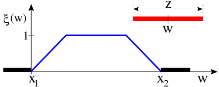
In the latter case, the maximum probability of adsorption is achieved for $w=\frac{x_{1}+x_{2}}{2}$, for which $\xi(w)=\frac{x}{z}$. The formulas (3.2) and (3.3) give the same probability density function $\xi(\cdot)$ for $z=x$ as is desirable. The plot of $\xi$ as a function of $w$ is given in Figure 1.

(a)   (b)

Figure 1: The probability $\xi$ as a function of $w$ for gRSA model $(\ref{defxi1})$ – $(\ref{defxi2})$: (a) for the case $z\leq x=x_{2}-x_{1}$; (b) for the case $z>x=x_{2}-x_{1}$.

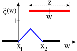
Formula (3.2) is shown in Figure 1(a) where the gap size $x=x_{2}-x_{1}$ is greater than the length of the new polymer segment $z$. Formula (3.3) is shown in Figure 1(b) where the gap size $x=x_{2}-x_{1}$ is less than the length of the new polymer $z$.

To explain the motivation behind formula (3.2), three possible cases of the relative position of the new (red) interval of the length $z\leq x$ and the gap $(x_{1},x_{2})$ are shown in Figure 2.

(a)​​​​​    (b)​​​​​​​​​​​​    (c)​​​​​​​​​​​​

Figure 2: Schematic of gRSA. (a) Polymer is refused; (b) polymer is adsorbed with the probability $\xi(z,w-x_{1},x_{2}-w)$; (c) polymer is adsorbed.

In Figure 2(a), the red interval is rejected because its middle point $w$ lies inside a polymer segment which is already adsorbed to the surface. Hence, the probability of adsorption is $0$, the same probability as in the classical RSA model. In Figure 2(c), the red segment of the length $z$ does not overlap with neighbouring polymers, and we allow it to be adsorbed with probability $\xi=1$. Cases in Figure 2(a) and Figure 2(c) are treated as in the classical RSA model.

In Figure 2(b), the center of the red polymer is inside the gap but the red polymer overlaps with neighboring polymers segments. This polymer would be rejected by the classical RSA model. We believe it is more realistic to consider that such a polymer will be adsorbed with some nonzero probability which continuously interpolates between the cases shown in Figures 2(a) and 2(c), i.e. between zero for $w-x_{1}=0$ and 1 for $w-x_{1}=z$. Formula (3.2) takes this fact into account, using simple linear interpolation. Formula (3.3) naturally extends the formula (3.2) for polymer segment lengths greater than the gaps (see also Figure 1).

Having explained the new rules for adsorbing the polymer, we must also specify what part of the surface is actually covered. We will assume that the new polymer covers only the intersection of the intervals

$$\left[w-\frac{z}{2},w+\frac{z}{2}\right]\bigcap\left[x_{1},x_{2}\right].$$ (3.4)

This guarantees that a possibly long, newly adsorbed polymer will not “spill over” and cover any part of the neighboring gaps.

4 Analysis of gRSA

Let $G(x,t)$ be the concentration of gaps (holes) of length $x$ at time $t$ and let $C(x,t)$ be the corresponding cumulative probability distribution function; that is,

$$C(x,t)=\frac{1}{\int_{0}^{\infty}G(y,t)\mbox{d}y}\int_{0}^{x}G(y,t)\mbox{d}y.$$ (4.1)

The total length of the surface that is covered by polymers at time $t$, $A(t)$, is directly related to $G(x,t)$ by

$$A(t)=1-\int_{0}^{1}xG(x,t)\mbox{d}x.$$ (4.2)

The number of polymers attached to the surface at time $t$, $N(t)$, can be also related to $G(x,t)$, as we will see in Section 4.1. Thus, the starting point of the analysis of the system is the derivation of the evolution equation for the distribution function of gaps $G(x,t)$.

A gap of length $x$ can be created from a larger gap (of length $y>x$) by adsorbing a suitable interval to the system. Thus the evolution of the concentration of gaps $G(x,t)$ is given by the equation

$$\frac{\partial G}{\partial t}(x,t) = -\;G(x,t)\int_{0}^{\infty}\left[\int_{0}^{x}\xi(z,u,x-u)\mbox{d}u\right]p(z)\mbox{d}z\;+$$

$$+\int_{x}^{\infty}\left[\int_{0}^{2(y-x)}2\,\xi\left(z,x+\frac{z}{2},y-x-\frac{z}{2}\right)p(z)\mbox{d}z\right]G(y,t)\mbox{d}y.$$

Using (3.2) and (3.3), equation (4) can be rewritten in the following form

$$\frac{\partial G}{\partial t}(x,t)=-G(x,t)\int_{0}^{x}\left[\int_{0}^{z/2}\frac{2u}{z}\mbox{d}u+\int_{z/2}^{x-z/2}1\,\mbox{d}u+\int_{x-z/2}^{x}\frac{2(x-u)}{z}\mbox{d}u\right]p(z)\mbox{d}z-$$

$$-G(x,t)\int_{x}^{\infty}\left[\int_{0}^{x/2}\frac{2u}{z}\mbox{d}u+\int_{x/2}^{x}\frac{2(x-u)}{z}\mbox{d}u\right]p(z)\mbox{d}z+$$ (4.4)

$$+\int_{x}^{\infty}\int_{0}^{y-x}2G(y,t)p(z)\mbox{d}z\mbox{d}y+\int_{x}^{\infty}\int_{y-x}^{2(y-x)}2\frac{2(y-x)-z}{z}G(y,t)p(z)\mbox{d}z\mbox{d}y.$$

Hence,

$$\frac{\partial G}{\partial t}(x,t)=-G(x,t)\int_{0}^{x}\left[x-\frac{z}{2}\right]p(z)\mbox{d}z-G(x,t)\int_{x}^{\infty}\left[\frac{x^{2}}{2z}\right]p(z)\mbox{d}z+$$ (4.5)

$$+\int_{x}^{\infty}\int_{0}^{y-x}2G(y,t)p(z)\mbox{d}z\mbox{d}y+\int_{x}^{\infty}\int_{y-x}^{2(y-x)}2\left[\frac{2(y-x)}{z}-1\right]G(y,t)p(z)\mbox{d}z\mbox{d}y.$$

We assume that the lengths of polymers are distributed according to formula (3.1) for $\alpha>-1$ and small $\varepsilon\ll 1.$ Moreover, we assume that there are already no holes of the length greater than $\varepsilon/2$ in the system, i.e. $G(x,t)=0$ for $x>\varepsilon/2.$ Then (using (3.1)), equation (4.5) can be rewritten (for $x<\varepsilon/2$ and $\alpha\neq 0$) as

$$\frac{\partial G}{\partial t}(x,t)=-\frac{G(x,t)(\alpha+1)}{\varepsilon^{\alpha+1}}\int_{0}^{x}\left[x-\frac{z}{2}\right]z^{\alpha}\mbox{d}z-\frac{G(x,t)(\alpha+1)}{\varepsilon^{\alpha+1}}\int_{x}^{\varepsilon}\left[\frac{x^{2}}{2z}\right]z^{\alpha}\mbox{d}z+$$

$$+\frac{2(\alpha+1)}{\varepsilon^{\alpha+1}}\int_{x}^{\infty}G(y,t)\int_{0}^{y-x}z^{\alpha}\mbox{d}z\mbox{d}y+$$

$$+\frac{2(\alpha+1)}{\varepsilon^{\alpha+1}}\int_{x}^{\infty}G(y,t)\int_{y-x}^{2(y-x)}\left[\frac{2(y-x)}{z}-1\right]z^{\alpha}\mbox{d}z\mbox{d}y$$

which implies

$$\frac{\partial G}{\partial t}(x,t)=\frac{x^{\alpha+2}G(x,t)}{\alpha(\alpha+2)\varepsilon^{\alpha+1}}-\frac{x^{2}G(x,t)(\alpha+1)}{2\alpha\varepsilon}+\frac{2^{\alpha+2}-4}{\alpha\varepsilon^{\alpha+1}}\int_{x}^{\infty}G(y,t)(y-x)^{\alpha+1}\mbox{d}y.$$ (4.6)

If $\alpha=0$, equation (4.5) implies (for $x<\varepsilon/2$)

$$\frac{\partial G}{\partial t}(x,t)=-\frac{x^{2}G(x,t)}{2\varepsilon}\left(\frac{3}{2}+\ln\left[\frac{\varepsilon}{x}\right]\right)+\frac{4\ln 2}{\varepsilon}\int_{x}^{\infty}G(y,t)(y-x)\mbox{d}y.$$ (4.7)

Equation (4.6) (or (4.7)) is the desired integro-differential equation for $G(x,t)$. If we solve (4.6), we can compute the evolution of $A(t)$ by (4.2). The equation for the evolution of $N(t)$ is given in the next section.

4.1 Evolution of $N(t)$

At each time step, an interval of length between $(z,z+\mbox{d}z)$ is chosen with probability $p(z)\mbox{d}z.$ This interval can be placed in any gap of size $x$ with probability $\int_{0}^{x}\xi(z,u,x-u)\mbox{d}u.$ There exist $G(x,t)\mbox{d}x$ gaps whose size lies in the interval $(x,x+\mbox{d}x).$ Hence, the integral $\int_{0}^{\infty}[\int_{0}^{x}\xi(z,u,x-u)\mbox{d}u]G(x,t)\mbox{d}x$ gives the probability that the randomly chosen position of the polymer of length $z$ will be accepted. Thus the probability of attaching a polymer of any length at one time step is equal to

$$\int_{0}^{\infty}\int_{0}^{\infty}\left[\int_{0}^{x}\xi(z,u,x-u)\mbox{d}u\right]G(x,t)p(z)\mbox{d}x\mbox{d}z.$$ (4.8)

Using a continuous approximation for $N(t)$, we find that $N(t)$ satisfies the following ordinary differential equation

$$\frac{\mbox{d}N}{\mbox{d}t}=\int_{0}^{\infty}\int_{0}^{\infty}\left[\int_{0}^{x}\xi(z,u,x-u)\mbox{d}u\right]G(x,t)p(z)\mbox{d}z\mbox{d}x.$$ (4.9)

Taking $p(z)$ to be given by (3.1) and $\xi(z,u,x-u)$ to be given by (3.2) – (3.3), and considering the regime where all gaps are already less than $\varepsilon$ (i.e. $G(x,t)=0$ for $x>\varepsilon$), we obtain

$$\int_{0}^{\infty}\int_{0}^{\infty}\left[\int_{0}^{x}\xi(z,u,x-u)\mbox{d}u\right]G(x,t)p(z)\mbox{d}z\mbox{d}x=$$

$$\int_{0}^{\infty}\int_{0}^{x}\left[\int_{0}^{z/2}\frac{2u}{z}\mbox{d}u+\int_{z/2}^{x-z/2}1\mbox{d}u+\int_{x-z/2}^{x}\frac{2(x-u)}{z}\mbox{d}u\right]G(x,t)p(z)\mbox{d}z\mbox{d}x+$$

$$+\int_{0}^{\infty}\int_{x}^{\infty}\left[\int_{0}^{x/2}\frac{2u}{z}\mbox{d}u+\int_{x/2}^{x}\frac{2(x-u)}{z}\mbox{d}u\right]G(x,t)p(z)\mbox{d}z\mbox{d}x=$$

$$=\int_{0}^{\varepsilon}G(x,t)\int_{0}^{x}\left[x-\frac{z}{2}\right]p(z)\mbox{d}z\mbox{d}x+\frac{1}{2}\int_{0}^{\varepsilon}G(x,t)x^{2}\int_{x}^{\infty}\frac{p(z)}{z}\mbox{d}z\mbox{d}x=$$

$$=\frac{\alpha+1}{\varepsilon^{\alpha+1}}\int_{0}^{\varepsilon}G(x,t)\int_{0}^{x}\left[x-\frac{z}{2}\right]z^{\alpha}\mbox{d}z\mbox{d}x+\frac{\alpha+1}{2\varepsilon^{\alpha+1}}\int_{0}^{\varepsilon}G(x,t)x^{2}\int_{x}^{\varepsilon}z^{\alpha-1}\mbox{d}z\mbox{d}x=$$

$$=-\frac{1}{\alpha(\alpha+2)\varepsilon^{\alpha+1}}\int_{0}^{\varepsilon}G(x,t)x^{\alpha+2}\mbox{d}x+\frac{\alpha+1}{2\alpha\varepsilon}\int_{0}^{\varepsilon}G(x,t)x^{2}\mbox{d}x.$$

Hence

$$\frac{\mbox{d}N}{\mbox{d}t}=-\frac{1}{\alpha(\alpha+2)\varepsilon^{\alpha+1}}\int_{0}^{\varepsilon}G(x,t)x^{\alpha+2}\mbox{d}x+\frac{\alpha+1}{2\alpha\varepsilon}\int_{0}^{\varepsilon}G(x,t)x^{2}\mbox{d}x.$$ (4.10)

Before analyzing (4.6) and (4.10) further, we summarize some results from the literature on classical RSA.

4.2 Some results for the classical RSA

If we consider particles of the same length $\varepsilon$ so that $p(z)=\delta(z-\varepsilon)$, and if we choose $\xi(z,w-x_{1},x_{2}-w)$ of the form

$$\xi(z,w-x_{1},x_{2}-w)=\left\{\begin{array}[]{ll}1\raisebox{-10.243pt}{\rule{0.0pt}{22.76219pt}}&\mbox{for}\;\;x_{1}+\displaystyle\frac{z}{2}\leq w\leq x_{2}-\displaystyle\frac{z}{2};\\ 0\raisebox{-7.39772pt}{\rule{0.0pt}{22.76219pt}}&\mbox{otherwise};\end{array}\right.$$ (4.11)

then our gRSA algorithm reduces to the classical RSA algorithm. The evolution equation (4) can be used to verify known one-dimensional results about fixed segment size, non-overlapping random sequential adsorption [10], namely one can show that the jamming limit is asymptotically approached as $t^{-1}$ [13].

Random sequential adsorption with a probability distribution $p(z)$ given by (3.1) and probability $\xi(z,w-x_{1},x_{2}-w)$ given by (4.11) has been studied in [10]. Then equation (4) for $x<\varepsilon$ reads as follows (assuming that initially there exist no holes of length greater than $\varepsilon$ in the system, i.e. $G(x,t)=0$ for $x>\varepsilon$)

$$\frac{\partial G}{\partial t}(x,t)=-\frac{x^{\alpha+2}G(x,t)}{(\alpha+2)\varepsilon^{\alpha+1}}+\frac{2}{\varepsilon^{\alpha+1}}\int_{x}^{x+\varepsilon}G(y,t)(y-x)^{\alpha+1}\mbox{d}y.$$ (4.12)

The scaling ansatz [10] for the concentration $G(x,t)$ can be written as

$$G(x,t)\sim t^{a}\Phi\left(x\,t^{b}\,\right)\quad\mbox{for}\quad x\ll 1,\quad t\gg 1,\quad\mbox{and}\quad xt^{b}\;\mbox{finite}.$$ (4.13)

Defining the moments

$$M_{\gamma}(t)=\int_{0}^{\infty}x^{\gamma}G(x,t)\mbox{d}x,\qquad m_{\gamma}=\int_{0}^{\infty}\xi^{\gamma}\Phi(\xi)\mbox{d}\xi$$ (4.14)

and using (4.13), we obtain

$$M_{\gamma}(t)\sim t^{a-b-b\gamma}m_{\gamma}.$$ (4.15)

Moreover, multiplying equation (4.12) by $x^{\gamma}$ and integrating over $x$, one can derive the equation for moments,

$$\frac{\partial M_{\gamma}}{\partial t}(x,t)=\frac{F(\gamma,\alpha)}{\varepsilon^{\alpha+1}}M_{\gamma+\alpha+2}\quad\mbox{where}\quad F(\gamma,\alpha)=2B(\gamma+1,\alpha+2)-\frac{1}{\alpha+2},$$ (4.16)

where $B(\cdot,\cdot)$ is Beta function. We define the function $\widehat{\gamma}(\alpha)$ implicitly by the equation $F(\widehat{\gamma},\alpha)=0$. If $\gamma$ is equal to $\widehat{\gamma}(\alpha)$, then the moment $M_{\gamma}$ is independent of time. Hence, using (4.15), we obtain the relation $a=b+b\,\widehat{\gamma}(\alpha)$ between the coefficients of the scaling ansatz (4.13) and the parameter $\alpha$ of the model. Finally, substituting the scaling ansatz (4.13) in (4.12), we find that $b=(\alpha+2)^{-1}.$ Thus, the scaling of moments (4.15) can be rewritten in the form

$$M_{\beta}(t)\sim t^{\mu}\qquad\mbox{where}\quad\mu=\frac{\widehat{\gamma}(\alpha)-\beta}{\alpha+2}.$$ (4.17)

Using (4.2) and (4.17), we obtain

$$1-A(t)=\int_{0}^{1}xG(x,t)\mbox{d}x\sim t^{-\omega(\alpha)}\qquad\mbox{where}\quad\omega(\alpha)=\frac{1-\widehat{\gamma}(\alpha)}{\alpha+2}.$$ (4.18)

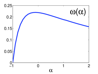
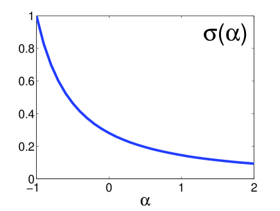
The graph of the function $\omega(\alpha)$ is given in Figure 3(a).

(a)   (b)

Figure 3: (a) The graph of the exponent $\omega(\alpha)$ given by $(\ref{scalingAt})$. (b) The graph of the exponent $\sigma(\alpha)$ given by $(\ref{scalingNt})$.

The equation (4.9) for $p(z)$ given by (3.1) and probability $\xi(z,w-x_{1},x_{2}-w)$ given by (4.11) reads as follows:

$$\frac{\mbox{d}N}{\mbox{d}t}=\frac{\varepsilon^{-\alpha-1}}{\alpha+2}\int_{0}^{\varepsilon}x^{\alpha+2}G(x,t)\mbox{d}x.$$ (4.19)

Using (4.17), we obtain (for $\sigma(\alpha)>0$)

$$N(t)\sim t^{\sigma(\alpha)}\qquad\mbox{where}\;\;\sigma(\alpha)=\frac{\widehat{\gamma}(\alpha)}{\alpha+2}.$$ (4.20)

The graph of the function $\sigma(\alpha)$ is given in Figure 3(b).

4.3 Evolution of gRSA

The temporal evolution of the gRSA model is more complex than the cases discussed in Section 4.2. To see this, we use the moments $M_{\gamma}(t)$ defined by (4.14). Multiplying equation (4.6) by $x^{\gamma}$ and integrating over $x$, we can derive the equation for moments (for $\alpha\neq 0$),

$$\frac{\partial M_{\gamma}}{\partial t}(x,t)=\frac{1}{\alpha(\alpha+2)\varepsilon^{\alpha+1}}M_{\gamma+\alpha+2}-\frac{\alpha+1}{2\alpha\varepsilon}M_{\gamma+2}\;+$$

$$+\;\int_{0}^{\infty}\frac{2^{\alpha+2}-4}{\alpha\varepsilon^{\alpha+1}}\int_{x}^{\infty}G(y,t)x^{\gamma}(y-x)^{\alpha+1}\mbox{d}y\mbox{d}x=$$

$$=\frac{1}{\alpha(\alpha+2)\varepsilon^{\alpha+1}}M_{\gamma+\alpha+2}-\frac{\alpha+1}{2\alpha\varepsilon}M_{\gamma+2}+\int_{0}^{\infty}\frac{2^{\alpha+2}-4}{\alpha\varepsilon^{\alpha+1}}G(y,t)\int_{0}^{y}x^{\gamma}(y-x)^{\alpha+1}\mbox{d}x\mbox{d}y=$$

$$=\frac{M_{\gamma+\alpha+2}}{\alpha(\alpha+2)\varepsilon^{\alpha+1}}+\frac{2^{\alpha+2}-4}{\alpha\varepsilon^{\alpha+1}}\int_{0}^{\infty}G(y,t)y^{\gamma+\alpha+2}\mbox{d}y\int_{0}^{1}\xi^{\gamma}(1-\xi)^{\alpha+1}\mbox{d}\xi-\frac{\alpha+1}{2\alpha\varepsilon}M_{\gamma+2}=$$

$$=\frac{1}{\varepsilon^{\alpha+1}}\left(\frac{2^{\alpha+2}-4}{\alpha}B(\gamma+1,\alpha+2)+\frac{1}{\alpha(\alpha+2)}\right)M_{\gamma+\alpha+2}-\frac{\alpha+1}{2\alpha\varepsilon}M_{\gamma+2}=$$

$$=\frac{1}{\varepsilon^{\alpha+1}}H(\gamma,\alpha)M_{\gamma+\alpha+2}-\frac{\alpha+1}{2\alpha\varepsilon}M_{\gamma+2},$$ (4.21)

where $B(\cdot,\cdot)$ is Beta function and $H(\gamma,\alpha)$ is defined as

$$H(\gamma,\alpha)=\frac{2^{\alpha+2}-4}{\alpha}B(\gamma+1,\alpha+2)+\frac{1}{\alpha(\alpha+2)}.$$ (4.22)

First, consider the case $\alpha<0$; the dominant term on the right-hand side of (4.21) is the term $\varepsilon^{-\alpha-1}H(\gamma,\alpha)M_{\gamma+\alpha+2}$. The zeroth order moment,

$$M_{0}(t)=\int_{0}^{\infty}G(x,t)\mbox{d}x,$$

gives the total number of gaps at time $t$. At leading order, we have

$$\frac{\partial M_{0}}{\partial t}(x,t)=\varepsilon^{-\alpha-1}H(0,\alpha)M_{\alpha+2}.$$

There is a constant $\overline{\alpha}\doteq-0.415$ such that $H(0,\alpha)$ is positive for $\alpha<\overline{\alpha}$ and negative for $\alpha>\overline{\alpha}$. We immediately see that

$$\int_{0}^{\infty}G(x,t)\mbox{d}x\quad\to\quad 0\qquad\qquad\mbox{for}\quad\alpha>\overline{\alpha}.$$ (4.23)

To illustrate the result (4.23), we will execute two stochastic simulations with the gRSA algorithm. We will use (3.1), (3.2) and (3.3) where $\alpha=-0.1$ or $\alpha=-0.3$. We choose $\varepsilon=10^{-3}$. The results are given in Figure 4, where the time evolution of the number of gaps and the number of adsorbed polymers are shown. Note that we use a logarithmic scale on the time axis because the long-term dynamics are very slow.

$\alpha=-0.1$             $\alpha=-0.3$

 

 

 

Figure 4: gRSA model for $\alpha=-0.1$ (panels on the left) and $\alpha=-0.3$ (panels on the right). We plot the time evolution of the number of adsorbed polymers (top panels) and the time evolution of the number of gaps (middle panels). The time axis of the top and middle panels is logarithmic. We also plot the time evolution of the quantity $[1-A(t)]^{-1}$ (bottom panels) where time is scaled according to $(\ref{scalingAtgenRSA})$.

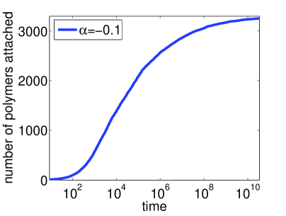
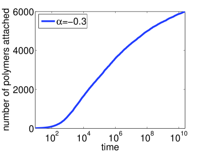
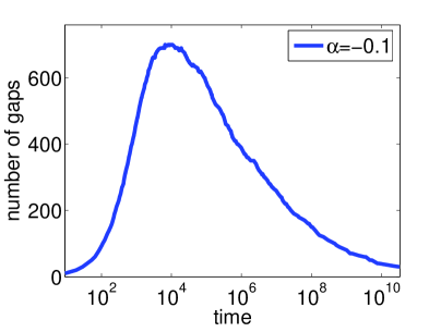
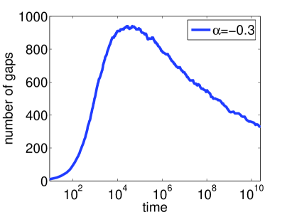
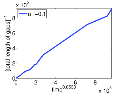
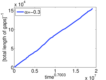
For $\alpha=-0.1$, the stochastic simulation was stopped when $99.9999\%$ of the surface was covered. For $\alpha=-0.3$, the stochastic simulation was stopped when $99.9994\%$ of the surface was covered.

Next, we will study the behaviour of the system for $\alpha<\overline{\alpha}$. Here, we will assume the scaling ansatz (4.13). Differentiating (4.22) with respect of $\gamma$, we obtain

$$\frac{\partial H}{\partial\gamma}(\gamma,\alpha)=\frac{2^{\alpha+2}-4}{\alpha}B(\gamma+1,\alpha+2)\Big{[}\psi_{0}(\gamma+1)-\psi_{0}(\gamma+\alpha+3)\Big{]}$$ (4.24)

where $\psi_{0}$ is the polygamma function. For each $\alpha<\overline{\alpha}$, the equation

$$H(\overline{\gamma},\alpha)=0$$ (4.25)

defines implicitly the function $\overline{\gamma}(\alpha)$. If $\gamma$ is equal to $\overline{\gamma}(\alpha)$, then the moment $M_{\gamma}$ is independent of time. Hence, using (4.15), we obtain the relation

$$a=b+b\,\overline{\gamma}(\alpha)$$

between the coefficients of the scaling ansatz (4.13) and the parameter $\alpha$ of the model. Finally, substituting the scaling ansatz (4.13) into (4.21), one can find that $b=(\alpha+2)^{-1}.$ Hence, the scaling of moments (4.15) can be rewritten in the form

$$M_{\beta}(t)\sim t^{\overline{\mu}}\qquad\mbox{where}\quad\overline{\mu}=\frac{\overline{\gamma}(\alpha)-\beta}{\alpha+2}.$$ (4.26)

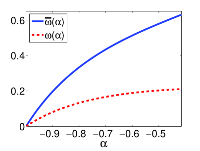
Using (4.2) and (4.26), we obtain

$$1-A(t)=\int_{0}^{1}xG(x,t)\mbox{d}x\sim t^{-\overline{\omega}(\alpha)}\qquad\mbox{where}\quad\overline{\omega}(\alpha)=\frac{1-\overline{\gamma}(\alpha)}{\alpha+2}.$$ (4.27)

The graph of the function $\overline{\omega}(\alpha)$ is given in Figure 5(a). We also plot $\omega(\alpha)$ given by (4.18) for comparison.

(a)   (b)

Figure 5: (a) The graph of the exponent $\overline{\omega}(\alpha)$ given by $(\ref{scalingAtgenRSA})$. The dashed line shows the exponent $\omega(\alpha)$ given by $(\ref{scalingAt})$. (b) The graph of the exponent $\overline{\sigma}(\alpha)$ given by $(\ref{scalingNtgenRSA})$. The dashed line shows the exponent $\sigma(\alpha)$ given by $(\ref{scalingNt})$.

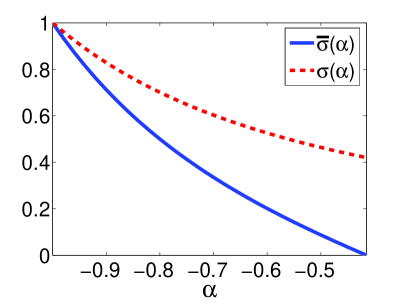
Using (4.10) and (4.26), we also obtain

$$N(t)\sim t^{\overline{\sigma}(\alpha)}\qquad\mbox{where}\;\overline{\sigma}(\alpha)=\frac{\overline{\gamma}(\alpha)}{\alpha+2}.$$ (4.28)

The graph of the function $\overline{\sigma}(\alpha)$ is given in Figure 5(b); we also plot $\sigma(\alpha)$ given by (4.20) for comparison.

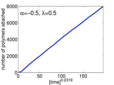
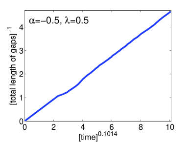
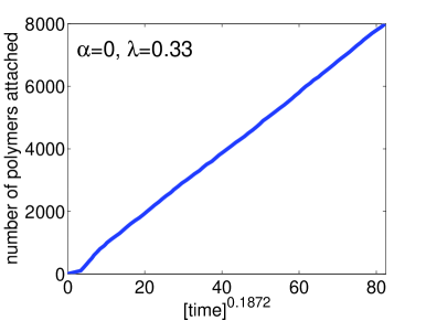
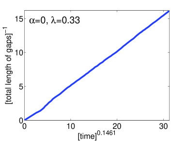
To illustrate the results (4.27) and (4.28), we will execute two gRSA stochastic simulations. We will use (3.1), (3.2) and (3.3) where $\alpha=-0.5$ or $\alpha=-2/3$. We choose $\varepsilon=10^{-3}$. The results are given in Figure 6 where the time evolution of the number of gaps and the number of adsorbed polymers are shown. The time is scaled according to (4.27) and (4.28); we solve (4.25) to obtain the desired exponents

$$\overline{\sigma}(-0.5)=0.0872,\quad\overline{\omega}(-0.5)=0.5795,\quad\overline{\sigma}\left(-\frac{2}{3}\right)=0.2875,\quad\overline{\omega}\left(-\frac{2}{3}\right)=0.4625,$$ (4.29)

and then we plot the results of stochastic simulations using the corresponding scaling (4.29).

$\alpha=-\displaystyle\frac{1}{2}$               $\alpha=-\displaystyle\frac{2}{3}$

 

 

 

Figure 6: gRSA model for $\alpha=-0.5$ (panels on the left) and $\alpha=-2/3$ (panels on the right). We plot the time evolution of the number of adsorbed polymers (top panels) and the time evolution of the inverse gap size $[1-A(t)]^{-1}$ (middle panels). Time is scaled according to $(\ref{scalingexample})$ (top and middle panels). We also plot the cumulative distribution function $C(x,t)$ at different times for both simulations (bottom panels).

$\alpha=-\displaystyle\frac{1}{2}$               $\alpha=-\displaystyle\frac{2}{3}$

 

Figure 7: Scaled cumulative distribution function of gaps for gRSA model for $\alpha=-0.5$ (panel on the left) and $\alpha=-2/3$ (panel on the right).

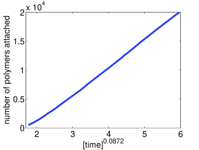
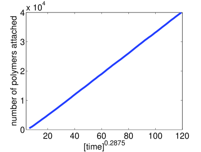
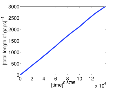
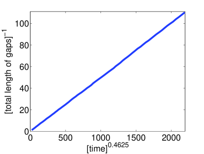
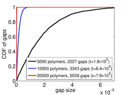
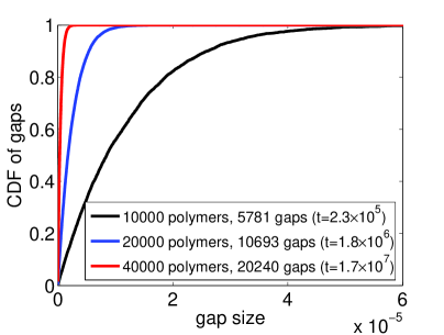
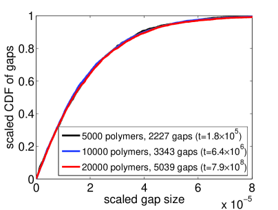
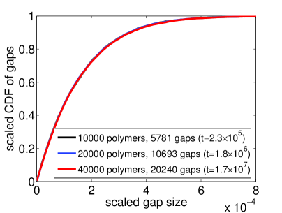
In Figure 6, we also plot the cumulative distribution function $C(x,t)$ for different times (i.e. for different numbers of polymers attached). Using the suitable rescaling $\widehat{C}(x,t)=C(kx,t)$, the curves collapse to a single curve as shown in Figure 7.

Finally, one can easily show that formula (4.27) works also for the case $\overline{\alpha}\leq\alpha<0.$ To illustrate it, we plot the time evolution of the quantity $[1-A(t)]^{-1}$ for $\alpha=-0.1$ and $\alpha=-0.3$ in Figure 4 (bottom panel) using the scaling (4.27). On the other hand, formula (4.28) is no longer correct because integrating of (4.10) implies that $N(t)$ is approaching a constant value. More precisely, $N(t)\sim C+t^{\overline{\sigma}(\alpha)}$ for $\overline{\sigma}(\alpha)<0.$ If $\alpha$ is positive than (4.23) is valid, i.e. we have (4.23) for any $\alpha>\overline{\alpha}$.

4.4 Time dependent concentration of reactive polymers

As discussed before, the reactive groups on our polymers are capable of reacting with the solvent before reaching the surface [15]. It may therefore be more realistic to consider that only a fraction of polymers $r(t)$ is still reactive at time $t$. Here, $r(t)\in[0,1]$, $r(0)=1$ and $r(t)$ is a decreasing function of time.

The random sequential adsorption algorithm has to be modified as follows: at each time step, we generate the random number uniformly distributed in the interval $(0,1)$. If this number is greater than $r(t)$, then the selected polymer has lost its binding site through reaction with the solvent (it cannot be adsorbed), and we continue with the next step. Otherwise, we choose randomly a position on the interval and we attempt to place the polymer there.

Depending on the form of function $r(t)$, different dynamics can be observed. First, let us suppose that

$$r(t)=\frac{1}{t^{\lambda}}\qquad\mbox{for}\;\lambda\in[0,1).$$ (4.30)

In this case, we can find a relation between the modified random sequential algorithm and the previous results. At each time $t$, we can compute the average waiting time $\Delta t$ before a reactive polymer hits the surface as the solution of the equation

$$\int_{t}^{t+\Delta t}\frac{1}{\tau^{\lambda}}\;\mbox{d}\tau=1.$$ (4.31)

Solving (4.31), we find

$$(t+\Delta t)^{1-\lambda}=t^{1-\lambda}+1-\lambda.$$

Hence,

$$\Delta t=\Big{[}t^{1-\lambda}+1-\lambda\Big{]}^{1/(1-\lambda)}-\,t\quad\sim\quad t^{\lambda}.$$

Consequently, we can make use of the formulas (4.18) and (4.20), or formulas (4.27) and (4.28), in the case (4.30). For example, using (4.18) and (4.20), we obtain that the quantities $A(t)$ and $N(t)$ satisfy the following asymptotic behaviour

$$A(t)\sim t^{(1-\lambda)\omega(\alpha)}\qquad\mbox{and}\qquad N(t)\sim t^{(1-\lambda)\sigma(\alpha)}.$$ (4.32)

To illustrate the formula (4.32), we stochastically simulate the gRSA model with the probability distribution $p(z)$ given by (3.1) and the probability $\xi(z,w-x_{1},x_{2}-w)$ given by (4.11), where the fraction of the reactive polymers in the system decreases with time according to (4.30). We select $\varepsilon=10^{-3}$ and verify the asymptotic behaviour (4.32) for $\alpha=-0.5$ and $\lambda=0.5$. Then (4.32) implies

$$1-A(t)\sim t^{-0.1014}\qquad\mbox{and}\qquad N(t)\sim t^{0.2319}.$$

The time evolution of $A(t)$ and $N(t)$ is given in Figure 8 (top panels). We also present results for $\alpha=0$ and $\lambda=0.33$ in Figure 8 (bottom panels). Again, we scale the time according to (4.32).

  

  

Figure 8: Modified RSA model from Section $\ref{sectimedependent}.$ The time evolution of the number of polymer molecules attached to the surface $N(t)$ (left). Time evolution of the inverse of the total gap size $[1-A(t)]^{-1}$ (right). Time is scaled according to $(\ref{scalingANtlambda})$.

The reactive group is lost by chemical reaction with the solvent. It might be more natural to consider (instead of (4.30)) that the fraction of reactive polymers is exponentially decreasing, i.e.

$$r(t)=e^{-\lambda t}\qquad\mbox{for}\;\lambda>0.$$ (4.33)

The formula (4.33) gives rise to qualitatively different dynamics for the system, as opposed to the dynamics associated with (4.30). For simplicity, let us assume that every polymer with a functional reactive group can be adsorbed (which will give a bound on $N(t)$ from above). Then the average number of adsorbed polymers $N(t)$ is

$$N(t)=\frac{1}{\lambda}\Big{(}1-e^{-\lambda t}\Big{)},$$

which implies that the number of adsorbed polymers does not approach infinity as in the previous case.

5 Equation-free analysis of gRSA

In the previous theory, we assumed the scaling ansatz (4.13) (see also [10]) for $G(x,t)$ and we computed the time dependence of the quantities of interest $A(t)$ and $N(t)$. A related interesting question is whether we can also compute the profile $\Phi$ from (4.13). One possibility is to substitute (4.13) in equation (4.6) and solve it numerically for $\Phi$ but we will not proceed this way. Instead, we demonstrate the computation of self-similar profile $\Phi$ using only short-time appropriately initialized simulations of the stochastic gRSA model. In this equation-free context [9, 2], it is easier to work with the cumulative distribution function $C(x,t)$, which can be obtained from $G(x,t)$ through (4.1); $C(x,t)$ is less noisy than $G(x,t)$ (e.g. [8]). Using (4.1) and (4.13), we obtain

$$C(x,t)=\frac{1}{\int_{0}^{\infty}G(y,t)\mbox{d}y}\int_{0}^{x}G(y,t)\mbox{d}y=$$

$$=\frac{1}{\int_{0}^{\infty}\Phi\left(y\,t^{b}\,\right)\mbox{d}y}\int_{0}^{x}\Phi\left(y\,t^{b}\,\right)\mbox{d}y=\frac{1}{\int_{0}^{\infty}\Phi\left(\xi\right)\mbox{d}\xi}\int_{0}^{xt^{b}}\Phi\left(\xi\right)\mbox{d}\xi.$$

Hence, we see that the cumulative density function $C(x,t)$ scales as

$$C(x,t)\equiv\overline{C}(xt^{b}).$$ (5.1)

To compute the profile $\overline{C}$, we can use an equation-free iterative fixed point algorithm which is shown schematically in Figure 9.

Figure 9: Schematic of the equation-free mapping $\Psi$.

Starting with the initial guess $\overline{C}_{0}$, we compute the sequence of profiles $\overline{C}_{K}$, $K=1,2,3,\dots$, where

$$\overline{C}_{K+1}=\Psi(\overline{C}_{K}),\qquad\mbox{for}\;K=0,1,2,3,\dots,$$ (5.2)

and where the mapping $\Psi$ is obtained as the composition of the following four steps:

(a) Given the cumulative density profile $\overline{C}_{K}$, create one or more microscopic realizations of gaps in the unit interval such that the initial cumulative density function is $C(\cdot,0)=\overline{C}_{K}$.

(b) Use the microscopic simulator (i.e. use the gRSA algorithm) for a short time $\Delta t.$

(c) Compute the new cumulative distribution function $C(\cdot,\Delta t)$ at time $\Delta t.$

(d) Rescale $C(\cdot,\Delta t)$ to compute $\overline{C}_{K+1}$.

One possible way to rescale $C(\cdot,\Delta t)$ is to compute the average gap size $a_{0}$ from $C(\cdot,0)$ and the average gap size $a_{\Delta t}$ from $C(\cdot,\Delta t)$. Then the $\overline{C}_{K+1}$ can be computed by

$$\overline{C}_{K+1}(x)=C\left(\frac{a_{\Delta t}}{a_{0}}x,\Delta t\right).$$ (5.3)

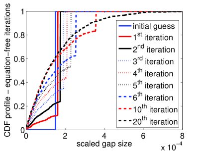
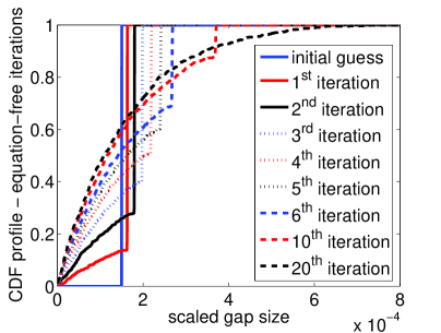
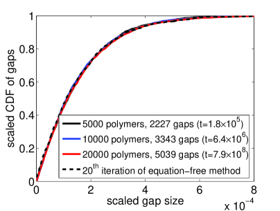
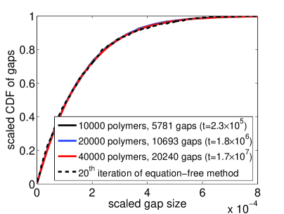
We now present illustrative results obtained by this fixed point computation (5.2) using the gRSA algorithm. We will use (3.1), (3.2) and (3.3) where $\alpha=-0.5$ or $\alpha=-2/3$. We choose $\epsilon=10^{-3}$. The results of long term simulations for these parameter values were already shown in Figure 6. Our goal is to use the iterative formula (5.2) to compute the scaled cumulative distribution function profile which was shown in Figure 7. This algorithm allows us to find the self-similar shape by performing simulations while simulating at a scale (at relatively larger average gap sizes) where the evolution is relatively fast, compared to the long-term dynamics close to jamming. The initial guess is given as

$$\overline{C}_{0}(x)=\left\{\begin{array}[]{ll}0&\mbox{for}\;x\leq 1.5\times 10^{-4};\\ 1&\mbox{for}\;x>1.5\times 10^{-4};\\ \end{array}\right.$$

which means that initially all our gaps have the same size $1.5\times 10^{-4}$. At each iteration step (see Figure 9), we place 1000 gaps according to the cumulative distribution function $\overline{C}_{K}$ to the interval $[0,1].$ We evolve the simulation until 100 new polymers are placed. We then rescale the new cumulative distribution according to (5.3) and we compute $\overline{C}_{K+1}$. Several first iterations are shown in Figure 10 (top panels). We see that after 20 iterations, we have effectively reached the steady state (the stationary shape of the self-similarly evolving gap distribution). More precisely, the error between iterations is small and it is not further systematically decreasing. The comparison of the equation-free 20th iteration with the results obtained by the long-time simulations are also shown in Figure 10 (bottom panels).

$\alpha=-\displaystyle\frac{1}{2}$               $\alpha=-\displaystyle\frac{2}{3}$

 

 

Figure 10: Equation free gRSA computational results for $\alpha=-0.5$ (left panels) and $\alpha=-2/3$ (right panels). Iterations of the equation-free dynamic renormalization algorithm $(\ref{formulapsi})$ (top panels). Comparison with the steady steate profile obtained through long time simulations (bottom panels).

Finally, we note that many other algorithmic possibilities for the computation of the profile $\overline{C}$ exist. The equation (5.2) seeks a fixed point of the mapping $\Psi$. Instead of successive substitution, other fixed point algorithms implemented in a matrix-free fashion through short simulation bursts can be used to find stationary solutions - for example, Newton-GMRES iterations [2]; these would be able to converge on even dynamically unstable self-similarly evolving distributions.

6 Discussion

In this paper, motivated by a pharmacological example involving polymer coating of a virus surface, we studied certain aspects of polydisperse adsorption of macromolecules in one spatial dimension. We presented an extension of the classical random sequential adsorption algorithm to capture better certain essential properties of the pharmacological model system currently used in drug development research. We introduced partial overlapping of adsorbing macromolecules, i.e. we considered that the polymers are not rigid objects but they can be deformed while attaching to the surface. We found two distinct asymptotic regimes. Depending on the parameters of the processes involved, we can observe that either (a) the number of gaps between polymers asymptotically approaches zero, or that (b) the number of gaps asymptotes to infinity and the gap distribution acquires an asymptotically self-similar profile.

We also briefly discussed the impact of a possible reaction of the polymers with the solvent on gRSA dynamics. Again, two possibilities exist. If the decay of the reactive groups is relatively weak, then the dynamics of the system remains qualitatively unchanged and the system only evolves on a slower time scale. On the other hand, if the reactive groups decay exponentially, this decay ultimately wins over the polynomial time asymptotics of gRSA. From the applications point of view, it therefore becomes crucial to know the corresponding rate constants in order to reliably predict what type of behaviour one might expect over the time scales of interest. Typically, the coating process is performed overnight in the laboratory and different reactive groups have different half lives; measuring these rates becomes an important task.

In this paper we worked in one spatial dimension and provided analytical results about the long time behaviour of gRSA models. The analytical approach was based on two important facts: we knew what the good macroscopic observables for describing the system behaviour were and we were able to write down analytically tractable equations for these observables. The good observable for our system was a distribution of gaps $G(x,t)$ between adsorbed polymers. If we know the initial distribution of gaps $G(0,t)$ one could easily predict $G(x,t)$ at future times.

On the other hand, if we know (hope) that the gap distribution $G(x,t)$ is a good observable for the system of interest but we do not know the evolution equation for $G(x,t)$, then it is still possible to use the equation-free methods [9]. The main idea of the equation-free methods is to use the short bursts of appropriately initialized microscopic/stochastic computations to estimate macroscopic quantities of interest on demand. Hence, if one does not have an explicit coarse-grained evolution equation for the system statistics, one can in principle avoid long, brute-force simulations. This might be the case for one-dimensional adsorption problems with more complicated microscopic evolution rules.

The situation becomes significantly more difficult in the higher dimensional case. Here, the analytical theory is far behind in development, and the literature contains mostly computational results. The first question for higher dimensional adsorption is the nature of the “good” coarse-grained observables for the system. Good observables (the variables in terms of which the unavailable effective model would be written) are necessary for developing a useful analytical theory. Knowing appropriate coarse-grained observables is also an important feature of equation-free algorithms. Having one-dimensional analogues in mind, we see that one needs an effective way to describe the statistics of “gaps” (free space) in higher dimensions. If we cannot estimate (by intuition or by suitable algorithms for the detection of low-dimensionality in high-dimensional data) effectively good observables for the system, then the direct, brute-force computationally intensive simulations might be the only modelling option. In this paper we showed cases where we could do more than brute-force simulation and provided analytical results giving insights into the dynamics of gRSA.

The problems studied in this paper were motivated by the pharmacological example mentioned above, and realistic predictive modelling of the problem clearly requires extensive model parameter information that must come from experimental data. As we showed, we can expect different dynamics of the problem depending on the values of the parameters of the polymer and the virus which are used. Obtaining reliably such parameters and bounds on their uncertainty for our particular model problem is non-trivial, and we are not yet ready to report about it.

References

- [1] N. Brilliantov, Y. Andrienko, P. Krapivsky, and J. Kurths, Fractal formation and ordering in random sequential adsorption, Physical Review Letters 76 (1996), no. 21, 4058–4061.
- [2] L. Chen, I. Kevrekidis, and P. Kevrekidis, Equation-free dynamic renormalization in a glassy compaction model, 4 pages, available as arXiv.org/cond-mat/0412773, 2005.
- [3] P. de Gennes, Conformations of polymers attached to an interface, Macromolecules 13 (1980), 1069–1075.
- [4] M. Doi, Introduction to Polymer Physics, Oxford University Press, 1996.
- [5] J. Evans, Random and cooperative sequential adsorption, Reviews of Modern Physics 65 (1993), no. 4, 1281–1329.
- [6] K. Fisher, Y. Stallwood, N. Green, K. Ulbrich, V. Mautner, and Seymour L., Polymer-coated adenovirus permits efficient retargeting and evades neutralising antibodies, Gene therapy 8 (2001), no. 5, 341–348.
- [7] K. Fisher, K. Ulbrich, V Subr, C. Ward, V. Mautner, D. Blakey, and Seymour L., A versatile system for receptor-mediated gene delivery permits increased entry of dna into target cells, enhanced delivery to the nucleus and elevated rates of transgene expression, Gene therapy 7 (2000), no. 15, 1337–1343.
- [8] C. Gear, Projective integration methods for distributions, NEC TR 2001-130 (2001), 1–9.
- [9] I. Kevrekidis, C. Gear, J. Hyman, P. Kevrekidis, O. Runborg, and K. Theodoropoulos, Equation-free, coarse-grained multiscale computation: enabling microscopic simulators to perform system-level analysis, Communications in Mathematical Sciences 1 (2003), no. 4, 715–762.
- [10] P. Krapivsky, Kinetics of random sequential parking on a line, Journal of statistical physics 69 (1992), no. 1/2, 135–150.
- [11] S. Milner, T. Witten, and M. Cates, Theory of the grafted polymer brush, Macromolecules 21 (1988), 2610–2619.
- [12] C. Pouton and L. Seymour, Key issues in non viral gene delivery, Advanced Drug Delivery Reviews 34 (1998), 3–19.
- [13] R. Swendsen, Dynamics of random sequential adsorption, Physical Review A 24 (1981), no. 1, 504–508.
- [14] S. Vorburger and K. Hunt, Adenoviral gene therapy, Oncologist (2002), no. 7, 46–59.
- [15] V. Šubr, Č. Koňák, R. Laga, and K. Ulbrich, Coating of DNA/Poly(L-lysine) complexes by covalent attachment of poly[N-(2-hydroxypropyl)methacrylamide], preprint, 31 pages, 2005.