Hidden Forces and Fluctuations from Moving Averages:
A Test Study

Abstract

The possibility that price dynamics is affected by its distance from a moving average has been recently introduced as new statistical tool. The purpose is to identify the tendency of the price dynamics to be attractive or repulsive with respect to its own moving average. We consider a number of tests for various models which clarify the advantages and limitations of this new approach. The analysis leads to the identification of an effective potential with respect to the moving average. Its specific implementation requires a detailed consideration of various effects which can alter the statistical methods used. However, the study of various model systems shows that this approach is indeed suitable to detect hidden forces in the market which go beyond usual correlations and volatility clustering.

, , , ,

1 Introduction

The concept of moving average is very popular in empirical trading algorithms bib1 but, up to now, it has received little attention from a scientific point of view bib2 , bib3 , bib4 . Recently we have proposed that a new definition of roughness can be introduced by considering fluctuations from moving averages with different time scales bib5 . This new definition seems to have various advantages with respect to the usual Hurst exponent in describing the fluctuations of high frequencies stock-prices.

A more specific analysis of these fluctuations can be found in two recent papers bib6 , bib7 which attempt to determine the tendency of the price to be attracted or repelled from its own moving average (Fig. 1). This is completely different from the use of moving averages in finance, in which empirical rules and predictions are defined in terms of a priori concepts bib1 . The idea is instead to introduce a statistical framework which is able to extract these tendencies from the price dynamics.

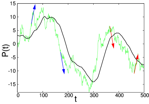
Figure 1: Example of a model of price dynamics (in this case a simple random walk) together with its moving average defined as the average over the previous $50$ points. The idea is that the distance of the price from its moving average can lead to repulsive (blue arrows) or attractive (red arrows) effective forces.

2 The Effective Potential Model

The basic idea is to describe price dynamics in terms of an active random walk (RW) which is influenced by its own moving average. This induces complex long range correlations which cannot be determined by the usual correlation functions and that can be explored by this new approach bib6 , bib7 . The basic ansatz is that price dynamics $P(t)$ can be described in terms of a stochastic equation of type:

$$P (t\!+\!\!1\!)\!-\!P(t)\!=$$ (1)

$$= \!-b(t)\frac{d}{d\Big{(}P(t)\!-\!P_{M}(t)\Big{)}}\Phi\Big{(}P(t)\!-\!P_{M}(t)\Big{)}\!+$$

$$+ \sigma(t)\omega(t)$$

where $\omega(t)$ corresponds to a random noise with unitary variance and

$$P_{M}(t)\equiv\frac{1}{M}\sum_{k=1}^{M}P(t-k)$$ (2)

is the moving average over the previous $M$ steps.

The potential $\Phi$ together with the pre-factor $b(t)$ describe the interaction between the price and the moving average. In both approaches bib6 , bib7 it is assumed to be quadratic:

$$\phi\Big{(}P(t)-P_{M}(t)\Big{)}={\Big{(}P(t)-P_{M}(t)\Big{)}}^{2}.$$ (3)

Despite this similar starting point the two studies proceed along rather different perspectives. In Ref. bib6 the three essential parameters of the model $(b;M;\sigma)$ are considered as constants with respect to $t$. Then, by analyzing the price fluctuations over a suitable time interval and for a long time series, the values of the three parameters are identified.

In Ref. bib7 instead the analysis is performed by looking directly at the relation between $P(t+1)-P(t)$ and $P(t)-P_{M}(t)$. This permits to derive the form of the potential and to identify the parameter $b(t)$ and its time variation. For the US$/Yen exchange rates the potential is found to be quadratic and it is possible to rescale it with the term $1/(M-1)$ observing a good data collapse. This would imply that it is not necessary to specify the time scale of the moving average.

3 Test Studies

Given these different perspectives, which arise from the same basic model, we decided to perform a series of tests of this approach which we present in this paper. We believe that these tests can elucidate various properties and limitations of the new approach and represent a useful information for its future developments and applications.

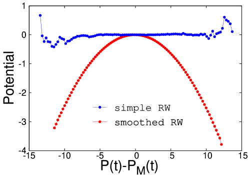
Figure 2: Effective potential for a random walk (flat line) and a smoothed random walk (convex parabola). The apparent repulsive potential corresponding to the smoothed RW is spurious and due to the correlations corresponding to the smoothing procedure. The units of the potential are defined by Eq.(1).

In Fig. 1 we show a simple RW and a moving average which represents its own smoothed profile. The analysis is performed by plotting the values of $P(t+1)-P(t)$ as a function of $P(t)-P_{M}(t)$ and deriving the potential by integrating from the center bib7 . The simple RW leads to a flat potential (no force) as expected (Fig. 2). Than we can take the smoothed profile (previous moving average) as a dataset by itself and repeat the analysis by comparing it to a new, smoother moving average (not shown). As one can see in Fig. 2 this leads to an apparent repulsive potential which should be considered as spurious.

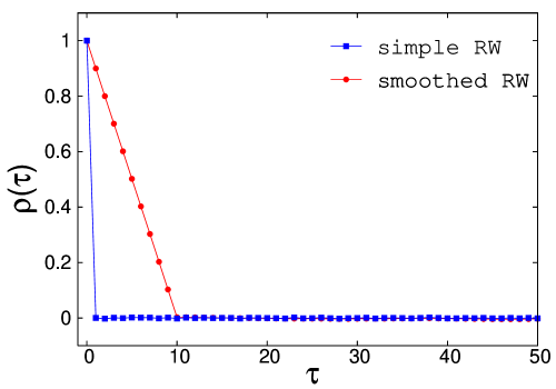
Figure 3: Autocorrelation ($\rho$) of the price increments for the simple RW and its smoothed profile. One can see that the smoothing procedure induces positive correlations up to the smoothing length (in this case $10$ steps).

This is due to the fact that the smoothed curve implies some positive correlations as shown in Fig. 3. Therefore in this framework positive correlations lead to a destabilizing potential with respect to the moving average.

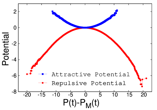
Figure 4: Effective potential reconstructed from a series of data obtained by a dynamics corresponding to Eqs.(1, 2) for the two cases of attractive and repulsive potentials. In this case $M=30$ and $b=\pm 1$. The units of the potential are defined by Eq.(1).

The opposite would happen for negative correlations (zig-zag behavior).

The interesting question is however if one can identify a non trivial situation in terms of the effective potential but in absence of simple correlations. This would be the new, interesting situation and the corresponding forces can be considered as hidden, in the sense that they do not have any effect in the usual correlation functions. Real stock-prices data clearly do not show any appreciable correlation, otherwise they would violate the simple arbitrage hypothesis. In the exchange rates instead there is a zig-zag behavior (negative correlation) at very short times which should be filtered with suitable methods in order to perform the potential analysis bib7 .

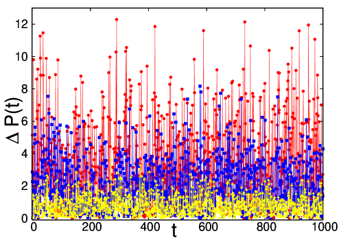
Figure 5: Absolute price variations for different time steps($\tau=1$ (yellow); $\tau=5$ (blue); $\tau=10$ (red)) corresponding to the dynamics of Eqs.(1, 2).

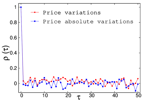
Figure 6: The correlation analysis of price variations shows no correlations between price differences and no volatility clustering effect. This implies that the presence of attractive or repulsive forces with respect to the moving averages is not detectable with the usual statistical indicators.

We now consider the model of the quadratic potential as in Refs. bib6 , bib7 . The effective potential is easily reconstructed as shown in Fig. 4. We also show in Fig. 5 the behavior of the absolute price variations for different time steps. The correlation function for the price and volatility are shown in Fig. 6 which clarifies that, in this case, no simple correlation is present, nor is there any volatility clustering effect. This is an interesting result because it shows that the new method is able to detect hidden forces which have no effect in the usual correlations of prices or volatility.

4 Probabilistic Models

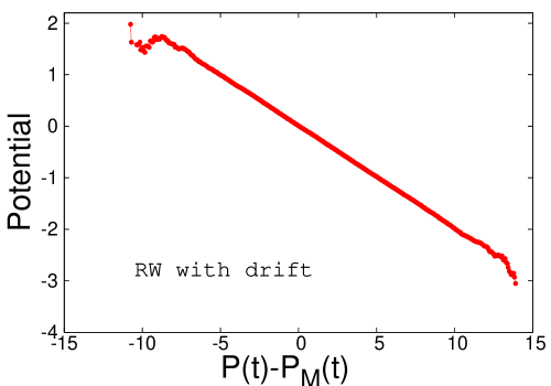
Figure 7: Effective potential corresponding to a RW with a constant drift which alters the probability for a step up or down. The units of the potential are defined by Eq.(1).

We now consider some variations to the RW which depend on $P(t)-P_{M}(t)$. We modify the probability of a certain step rather than the size of the step as in Eq.(1). The simplest model is to add a constant drift, independent on the value of $P_{M}(t)$. The effective potential corresponding to this case is simply linear as shown in Fig. 7. One can see that in this case the point where $P(t)-P_{M}(t)=0$ is not a special point and this model appears to be oversimplified with respect to the dataset analyzed up to now bib6 , bib7 .

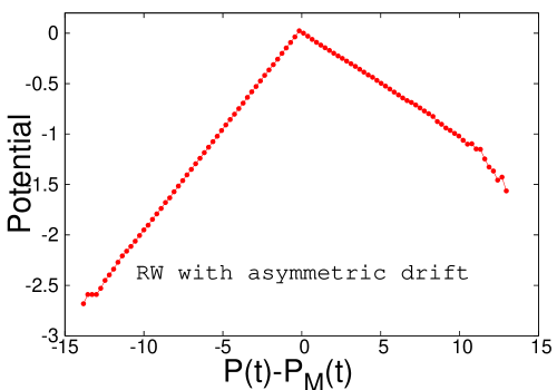
Figure 8: Effective potential corresponding to the dynamics of Eq.(6) with $\epsilon_{1}=0.05$ and $\epsilon_{2}=0.10$. One can see that in this case the distribution is asymmetric and it extends more in the direction for which the instability is stronger. In this model the effective force only depends on the sign of $P(t)-P_{M}(t)$ and not on its specific value. The units of the potential are defined by Eq.(1).

A more interesting model is represented by the following dynamics for a RW with only up and down steps:

$$\Bigg{\{}\begin{array}[]{ll}p(\uparrow)=1/2+\epsilon_{1}\;\;\;\mbox{for}\;\;\;P(t)-P_{M}(t)>0\\ p(\downarrow)=1/2-\epsilon_{1}\end{array}$$ (6)

$$\Bigg{\{}\begin{array}[]{ll}p(\uparrow)=1/2-\epsilon_{2}\;\;\;\mbox{for}\;\;\;P(t)-P_{M}(t)<0\\ p(\downarrow)=1/2+\epsilon_{2}\;.\end{array}$$

This implies a tendency of destabilization (repulsion from $P_{M}(t)$) whose strength is only dependent on the sign of $P(t)-P_{M}(t)$. In principle the situation can be asymmetric with $\epsilon_{1}\neq\epsilon_{2}$. The potential analysis for this case leads to a piecewise linear potential in which the slopes are related to $\epsilon_{1}$ and $\epsilon_{2}$ (Fig. 8).

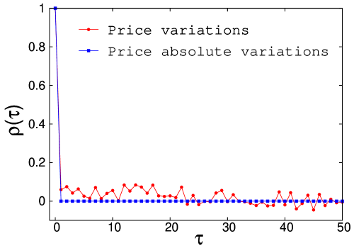
Figure 9: Correlation analysis of price variations and volatility for the model of Eq. (6). Also in this case no detectable correlations are present.

One can also see that one line extends more than the other indicating an asymmetric distribution. Also in this case the correlation of the price variations and volatilities show no detectable effect as shown in Fig. 9. Clearly in this case the effective potential is just a representation of the correlations between $P(t+1)-P(t)$ and $P(t)-P_{M}(t)$ whose microscopic origin is instead in the modification of the probability for unitary steps.

5 Fractal Model

It may be interesting to consider also the case of a fractal model constructed by an iterative procedure bib2 , Fig. 10.

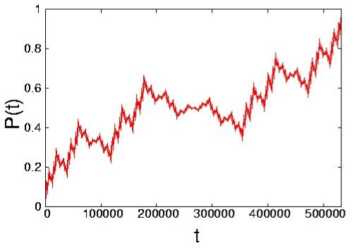
Figure 10: Example of a fractal model distribution of price

The fractal model does not have a specific dynamics but, since it is often considered as to capture some properties of real prices, we consider of some interest to study if this model would correspond to some type of effective potential. In Fig. 11 we can see that the effective potential is slightly attractive. Given the symmetry of the model construction, the asymmetry observed in the effective potential is probably due to the backward construction of the corresponding moving average.

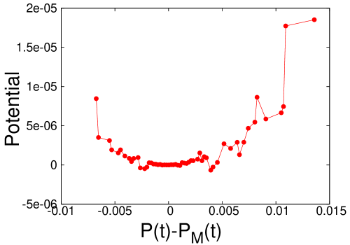
Figure 11: Effective potential corresponding to the fractal price model. The units of the potential are defined by Eq.(1).

6 Analysis of the Fluctuations

We now consider the nature of fluctuations from the moving average by analyzing the probability distribution $W\Big{(}P(t)-P_{M}(t)\Big{)}$ for the various models. In Fig. 12 we show the distributions corresponding to the quadratic potential as compared to that of a reference RW $(b=0)$. The first observation is that the repulsive potential makes the distribution broader (super diffusion) while the attractive potential makes it narrower (sub diffusion).

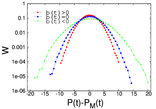
Figure 12: Distribution of the fluctuations, $W(P(t)-P_{M}(t))$, for the dynamics of Eq. (1-3) and different values of the parameter $b$.

This behavior was already observed in Refs. bib6 , bib7 . Less trivial is the fact that the distributions are well represented by gaussian curves.

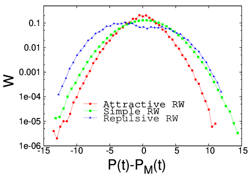
Figure 13: Distributions of the fluctuations, $W(P(t)-P_{M}(t))$, for the dynamics of Eq. (LABEL:eq14). In this case the distributions became asymmetric due to different values of ${\epsilon}_{1}$ and ${\epsilon}_{2}$.

In Fig. 13 we show the same distributions corresponding to the probabilistic model of Eq. (6) for the case of asymmetric attractive and repulsive effects. In this case there is a marked deviation from the gaussian behavior and the case of repulsive trend develops two separate peaks. It will be interesting to check the corresponding distribution on real stock-prices which we intend to perform in the future.

7 Conclusions and Perspectives

In summary the idea to consider price dynamics as influenced by an effective force dependent on the distance of price $P(t)$ from its own moving average $P_{M}(t)$ represents a new statistical tool to detect hidden forces in the market. The implementation of the analysis can be seriously affected by the eventual presence of positive or negative correlations. However, we have shown by a series of models and tests, that this new method is able to explore complex correlations which have no effect on the usual statistical tools like the correlations of price variation and the volatility clustering.

The method provides an analysis of the sentiment of the market: aggressive for the case of repulsive forces and conservative for attractive ones. In this respect it may represent a bridge between the financial technical analysis and the application of statistical physics to this field. In addition it may also be useful to analyze the results of the different strategies and behaviors which arise in agent based models.

References

- [1] B.J. Murphy, Technical Analysis of the Financial Markets, Prentice Hall Press, 1999.
- [2] B.B. Mandelbrot, Fractals and Scaling in Finance, Springer Verlag, New York, 1997.
- [3] R.N. Mantegna, H.E. Stanley, An Introduction to Econophysics, Cambridge University Press, Cambridge, 2000.
- [4] J.P. Bouchaud, Theory of Financial Risk and Derivative Pricing, Cambridge University Press, Cambridge, 2003.
- [5] V. Alfi, F. Coccetti, M. Marotta, A.Petri, L.Pietronero, Roughness and Finite Size Effect in the NYSE Stock-Price Fluctuations, preprint 2006.
- [6] VR. Baviera, M. Pasquini, J. Raboanary, M.Serva, Moving Averages and Price Dynamics, International Journal of Theoretical and Applied Finance, vol.5, num. 6, pag. 575-583, 2002.
- [7] M. Takayasu, T. Mizuno, H. Takayasu, Potentials of Unbalanced Complex Kinetics Observed in Market Time Series, http://arxiv.org/abs/physics/0509020.