Characterizing the reflectance near the Brewster angle: a Padé-approximant approach

Abstract

We characterize the reflectance peak near the Brewster angle for both an interface between two dielectric media and a single slab. To approach this problem analytically, we approximate the reflectance by a first-order diagonal Padé. In this way, we calculate the width and the skewness of the peak and we show that, although they present a well-resolved maximum, they are otherwise not so markedly dependent on the refractive index.

I Introduction

As it is well known, the behavior of the light reflected at the boundary between two dielectrics drastically depends on whether the associated electric field lies parallel ($p$ polarization) or perpendicular ($s$ polarization) to the plane of incidence. This is quantified by the Fresnel formulas BornWolf1999 , which also confirm that at a certain angle $\theta_{B}$ the $p$-polarized field drops to zero. This angle is commonly referred to as the Brewster angle and, in spite of its simplicity, it is a crucial concept in the optics of reflection Lekner1987 .

In fact, this notion is at the heart of a number of methods for optical thin-film characterization. These include Brewster-angle microscopy Honig1991 ; Henon1991 ; Lheveder1998 , which furnishes a direct visualization of the morphology of the film, or the Abelès Brewster-angle method Abeles1950 ; Traub1957 ; Hacskaylo1964 ; Heavens1991 ; Wu1993 for determining the refractive index. They are quite popular because are noncontact, easy to set up and simple to use. The basic idea can be concisely stated as follows: coated and bare regions of a substrate are illuminated with $p$-polarized light and the angle of incidence is scanned for a reflectance-match angle. Visual observation is often used because it reveals local variations in film thickness and in homogeneity of refractive index.

These techniques rely on the dependence of reflectance near the Brewster angle on the refractive indices involved. Of course, one could rightly argue that all the relevant information is contained in the Fresnel formulas. However, given their nonlinear features, no physical insights on the behavior around $\theta_{B}$ can be easily inferred, nor an analysis of the error sources can be easily carried out, except by numerical methods Burns1974 . Some qualitative comments can be found scattered in the literature: for example, it is sometimes argued that the amplitude reflection coefficient for $p$ polarization is approximately linear around $\theta_{B}$ Holmes1965 . Nevertheless, we think that a comprehensive study of the reflectance near the Brewster angle behavior is missing and it is precisely the main goal of this paper.

To this end, we propose to look formally at the reflectance as a probability distribution and focus on its central moments, which leads us to introduce very natural measures of the width and the skewness of that peak through the second and third moments Evans2000 . Since all these calculations must be performed only in a neighborhood of $\theta_{B}$, we replace the exact reflectance by a Padé approximant Baker1996 : apart from the elegance of this approach, it is sometimes mysterious how well this can work. In addition, we can then compute the relevant parameters in a closed way and deduce their variation with the refractive indices. This program is carried out in Section II for a single interface and in Section III for a homogeneous slab. Finally, our conclusions are summarized in Section IV.

II Behavior of the Brewster angle at an interface

Let two homogeneous isotropic semi-infinite dielectric media, described by real refractive indices $n_{0}$ and $n_{1}$, be separated by a plane boundary. We assume an incident monochromatic, linearly polarized plane wave from medium 0, which makes an angle $\theta_{0}$ with the normal to the interface and has amplitude $E^{(i)}$. This wave splits into a reflected wave $E^{(r)}$ in medium 0, and a transmitted wave $E^{(t)}$ in medium 1 that makes an angle $\theta_{1}$ with the normal. The angles of incidence $\theta_{0}$ and refraction $\theta_{1}$ are related by Snell’s law.

The wave vectors of all waves lie in the plane of incidence. When the incident fields are $p$ or $s$ polarized, all plane waves excited by the incident ones have the same polarization, so both basic polarizations can be treated separately. By demanding that the tangential components of $\mathbf{E}$ and $\mathbf{H}$ should be continuous across the boundary, and assuming nonmagnetic media, the reflection and transmission amplitudes are given by BornWolf1999

$$r_{s}&=\frac{E^{(r)}_{s}}{E^{(i)}_{s}}=\frac{n_{0}\cos\theta_{0}-n_{1}\cos\theta_{1}}{n_{0}\cos\theta_{0}+n_{1}\cos\theta_{1}},\\ \\ r_{p}=\frac{E^{(r)}_{p}}{E^{(i)}_{p}}=\frac{n_{1}\cos\theta_{0}-n_{0}\cos\theta_{1}}{n_{1}\cos\theta_{0}+n_{0}\cos\theta_{1}}.$$ (1)

These are the famous Fresnel formulas, represented in Fig. 1 and whose physical content is discussed in any optics textbook. The Brewster angle occurs when $r_{p}=0$, which immediately gives the condition

$$\theta_{B}=\tan^{-1}n,$$ (2)

where $n=n_{1}/n_{0}$ is the relative refractive index. Without loss of generality, in the rest of this section we assume $n_{0}=1$ and then $n=n_{1}$. Also, we deal exclusively with $p$ polarization and drop the corresponding subscript everywhere.

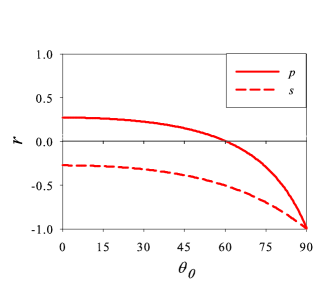
Figure 1: Plot of the amplitude reflection coefficients $r_{p}$ and $r_{s}$ as functions of the angle of incidence $\theta_{0}$ (in degrees) for an interface between air ($n_{0}=1$) and a homogeneous, isotropic dielectric medium ($n_{1}=1.75$).

To treat the reflectance

$$\mathfrak{R}=|r|^{2}$$ (3)

near the Brewster angle it proves convenient to use

$$\vartheta=\theta_{0}-\theta_{B},$$ (4)

which is the angle of incidence centered at $\theta_{B}$. Since we are interested only in a local study, we take into account only a small interval around $\theta_{B}$; that is, angles from $-\Delta\vartheta$ to $+\Delta\vartheta$. The length of this interval is largely an arbitrary matter: we shall take henceforth $\Delta\vartheta=15^{\circ}$, although the analysis is largely independent of this choice.

To quantify the peak near the Brewster angle, we treat the reflectance as a probability distribution in the interval $[-\Delta\vartheta,+\Delta\vartheta]$ and borrow some well-established concepts from statistics Evans2000 . In this manner we define

$$\bar{\vartheta}=\frac{\int_{-\Delta\vartheta}^{+\Delta\vartheta}d\vartheta\,\vartheta\ \mathfrak{R}(\vartheta)}{\int_{-\Delta\vartheta}^{+\Delta\vartheta}d\vartheta\,\mathfrak{R}(\vartheta)}.$$ (5)

For a symmetric peak $\bar{\vartheta}=0$, while the fact that $\bar{\vartheta}\neq 0$ reveals an intrinsic asymmetry.

The central moments are

$$\mu_{k}=\frac{\int_{-\Delta\vartheta}^{+\Delta\vartheta}d\vartheta\,\left(\vartheta-\bar{\vartheta}\right)^{k}\ \mathfrak{R}(\vartheta)}{\int_{-\Delta\vartheta}^{+\Delta\vartheta}d\vartheta\,\mathfrak{R}(\vartheta)},$$ (6)

and, as it happens for $\bar{\vartheta}$, they are functions of the refractive index $n$. The second moment is a measure of the width of the distribution, while the third moment can be immediately related with a lack of symmetry. More concretely, we take the width and the skewness of the Brewster peak as

$$w&=2\sqrt{\mu_{2}},\\ \\ \gamma=\frac{\mu_{3}}{\sqrt{\mu_{2}^{3}}}.$$ (7)

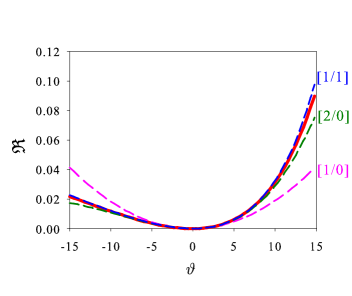
Figure 2: Reflectance (for $p$ polarization) of the same interface as in Fig. 1, but calculated in terms of the local angle of incidence $\vartheta$ (in degrees) for an interval $\pm\Delta\vartheta=15^{\circ}$. The exact reflectance is represented by the thick continuous line, while the broken lines are the Padé approximants in Eqs. (8). The corresponding orders $[L/M]$ are labeled in the right axis.

Of course, these parameters can be computed numerically by using the Fresnel formulas. However, since we are working in a small neighborhood of $\theta_{B}$, it seems more convenient to work with some local approximation to $r$ (and therefore to $\mathfrak{R}$). Here, we resort to Padé approximants (to maintain the paper as self-contained as possible, in the Appendix we briefly recall the essentials of such an approach). After some calculations, the approximations to the reflection coefficient $r$ turn out to be

$$r^{[1/0]}&=\frac{(1-n^{4})\vartheta}{2n^{3}},\\ r^{[2/0]}=\frac{(1-n^{4})\vartheta}{2n^{3}}\\ -\frac{(n^{8}+n^{6}+n^{4}-n^{2}-2)\vartheta^{2}}{4n^{6}},\\ r^{[1/1]}=\frac{(1-n^{4})\vartheta}{2n^{3}-(n^{4}+n^{2}+2)\vartheta},$$ (8)

whence one immediately gets the corresponding reflectances as $\mathfrak{R}^{[L/M]}=|r^{[L/M]}|^{2}$, which have been plotted in Fig. 2. As we can see, the term $\mathfrak{R}^{[1/0]}$ reproduces the exact reflectance only in a very small interval. The next polynomial approximation $\mathfrak{R}^{[2/0]}$ improves a little bit the situation, but fails again as soon we are, say $\pm 10^{\circ}$ away from $\theta_{B}$. On the contrary, the diagonal Padé $\mathfrak{R}^{[1/1]}$ fits remarkably well with the exact behavior. We thus conclude that $\mathfrak{R}^{[1/1]}$ provides an excellent approximation and we use it in subsequent calculations.

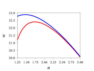
Figure 3: Width (in degrees) of the reflectance peak near the Brewster angle as a function of the refractive index $n$ for the same interface as in Fig. 1 (lower curve) and for a slab of index $n$ and thickness $d=\lambda/4$ (upper curve).

An additional and remarkable advantage of $\mathfrak{R}^{[1/1]}$ is that the central moments $\mu_{k}$ can be expressed in a closed analytical form. In Fig. 3 we have plotted the width $w$ as a function of the refractive index $n$ (lower curve). We have also computed $w$ by numerically integrating the Fresnel formulas: no appreciable differences can be noticed. The width has a maximum that can be calculated by imposing $dw/dn=0$, which immediately gives $n=\sqrt{3}$. Beyond this value, $w$ decreases almost linearly with $n$. However, for the range of indices plotted in the figure, this variation is smooth, with a total change in $w$ of around $3^{\circ}$.

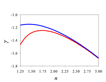
Figure 4: Skewness $\gamma$ of the reflectance peak near the Brewster angle as a function of the refractive index, for the same cases as in Fig. 3. The lower curve also corresponds to the interface, while the upper one if for the slab.

In Fig. 4 we have plotted the skewness $\gamma$ in terms of $n$. This parameter is always negative what, for a peak, means that the left tail is less pronounced than the right tail. There is again a maximum in the skewness that can be calculated by imposing $d\gamma/dn=0$. However, one can check that $\mu_{3}\simeq 1$ for all the values of $n$, so that $\gamma\simeq-8/w^{3}$: this maximum coincides then with that of $w$. Apart from a scale factor, $\gamma$ shows an aspect quite similar to that of $w$.

III Behavior of the Brewster angle at a single slab

We focus our attention now on a homogeneous, isotropic dielectric slab of refractive index $n$ and thickness $d$ imbedded in air and illuminated with monochromatic light (the case when the slab lies on a substrate can be dealt with much in the same way). A standard calculation gives the following amplitude reflection coefficient for the slab Azzam1987

$$R=\frac{r[1-\exp(-i2\beta)]}{1-r^{2}\exp(-i2\beta)},$$

where $r$ is the Fresnel reflection coefficient at the interface air-medium (which again will be considered for $p$ polarization only) and $\beta$ is the slab phase thickness

$$\beta=\frac{2\pi}{\lambda}d\sqrt{n^{2}-\sin^{2}\theta_{0}}.$$ (9)

Here $d$ is the thickness, $\lambda$ the wavelength in vacuo of the incident radiation and $\theta_{0}$ the angle of incidence. This coefficient $R$ presents a typical periodic variation with the slab phase thickness $\beta$. Apart from that dependence, it is obvious that $R=0$ when $r=0$; i. e., precisely at the Brewster angle for the interface air-medium. However, the form of this reflectance peak, calculated now as

$$\mathfrak{R}=|R|^{2},$$ (10)

differs from the case of a single interface, since (III) is more involved than (1). Although the analysis can be carried out for any value of $d$ such that $R\neq 0$, for definiteness and to avoid as much as possible any spurious detail, we take $d=\lambda/4$. In Fig. 5 we have plotted the exact form of the reflectance for this thickness, as a function of the local angle of incidence, defined as in Eq. (4), for several values of $n$

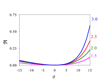
Figure 5: Reflectance (for $p$ polarization) of a slab of thickness $d=\lambda/4$ in terms of the local angle of incidence $\vartheta$, for various values of the refractive index (labeled in the right axis).

Instead of Eq. (III), we use again a Padé approximant of order $[1/1]$, which can be written as

$$R^{[1/1]}=\frac{p_{1}\vartheta}{1+q_{1}\vartheta}$$ (11)

where

$$p_{1}&=i\frac{1-n^{4}}{n^{3}}e^{-i\nu}\sin\nu,\\ \\ q_{1}=\frac{\nu}{n^{3}e^{i\nu}\sin\nu}-\frac{n^{4}+n^{2}+2}{2n^{3}},$$ (12)

and

$$\nu=\frac{2\pi n^{2}d}{\sqrt{n^{2}+1}}.$$ (13)

With this approximation, that still reproduces pretty well the exact reflectance, we have analytically obtained $w$ and $\gamma$ for the slab. The results are plotted in the upper curves of Figs. 3 and 4, respectively. For high values of $n$, the reflectance peak for the slab essentially coincides with that for the interface. Differences are only noticeable for small values of $n$. In fact, the maximum of $w$ can be evaluated by imposing $dw/dn=0$, whose numerical solution gives $n\simeq 1.45$. The behavior of $\gamma$ is quite similar, because here we have also that $\mu_{3}\simeq-1$ for all the values of $n$.

IV Conclusions

In summary, we have presented a simple and comprehensive treatment of the reflectance near the Brewster angle. By combining the notions of width and skewness with Padé approximants, we have fully characterized this reflectance peak. We hope that these results fill a gap for a full understanding of the Brewster angle.

Appendix: Padé approximants

A Padé approximant is a rational function (of a specified order) such that its power series expansion agrees with a given power series to the highest possible order. In other words, let us define

$$R^{[L/M]}(x)=\frac{P_{L}(x)}{Q_{M}(x)},$$ (A1)

where $P_{L}(x)$ and $Q_{M}(x)$ are polynomials of degrees $L$ and $M$, respectively:

$$P_{L}(x)&=p_{0}+p_{1}x+\ldots+p_{L}x^{L},\\ \\ Q_{M}(x)=1+q_{1}x+\ldots+q_{M}x^{M}.$$ (A2)

The rational function $R^{[L/M]}(x)$ is said to be a Padé approximant to the function $f(x)$, which has a Taylor expansion at $x=0$

$$f(x)=\sum_{k=0}^{\infty}f_{k}\ x^{k},$$ (A3)

if

$$&f(0)=R^{[L/M]}(0),\\ \\ \displaystyle\left.\frac{d^{k}}{dx^{k}}f(x)\right|_{x=0}=\left.\frac{d^{k}}{dx^{k}}R^{[L/M]}(x)\right|_{x=0},$$ (A4)

for $k=1,2,\ldots,L+M$. These conditions furnish $L+M+1$ equations for $p_{0},\ldots,p_{L}$ and $q_{1},\ldots,q_{M}$. The coefficients can be found by noticing that Eqs. (A4) are equivalent to

$$f(x)-\frac{P_{L}(x)}{Q_{M}(x)}=0,$$ (A5)

up to terms of order $L+M+1$. This gives directly the following set of equations:

$$f_{0}=p_{0},$$

$$f_{1}+f_{0}q_{1}=p_{1},$$

$$f_{2}+f_{1}q_{1}+f_{0}q_{2}=p_{2},$$

$$\;\vdots$$

$$f_{L}+f_{L-1}q_{1}+\ldots+f_{L-M+1}q_{M}=0,$$

$$\;\vdots$$

$$f_{L}+f_{L-1}q_{1}+\ldots+f_{L-M+1}q_{M}=0,$$

$$q_{L+M}+f_{L+M-1}q_{1}+\ldots+f_{L}q_{M}=0.$$ (A6)

Solving this directly gives

$$R^{[L/M]}(x)=\frac{\left|\begin{array}[]{cccc}f_{L-M+1}&f_{L-M+2}&\ldots&f_{L+1}\\ \vdots&\vdots&\ddots&\vdots\\ f_{L}&f_{L+1}&\ldots&f_{L+M}\\ \displaystyle\sum_{J=M}^{L}f_{J-M}\ x^{J}&\displaystyle\sum_{J=M-1}^{L}f_{J-M+1}\ x^{J}&\ldots&\displaystyle\sum_{J=0}^{L}f_{J}\ x^{J}\end{array}\right|}{\left|\begin{array}[]{cccc}f_{L-M+1}&f_{L-M+2}&\ldots&f_{L+1}\\ \vdots&\vdots&\ddots&\vdots\\ f_{L}&f_{L+1}&\ldots&f_{L+M}\\ x^{M}&x^{M-1}&\ldots&1\end{array}\right|}.$$ (A7)

Nevertheless, experience shows that Eqs. (Appendix: Padé approximants) are frequently close to singular, so that one should solve them by e. g. a full pivotal lower-upper triangular (LU) decomposition Numericalrecipes .

By contrast with techniques like Chebyshev approximation or economization of power series, that only condense the information that you already know about a function, Padé approximants can give you genuinely new information about your function values Numericalrecipes . We conclude by noting that, for a fixed value of $L+M$, the error is usually smallest when $L=M$ or when $L=M+1$.

References

- (1) M. Born and E. Wolf, Principles of Optics (Cambridge University Press, Cambridge, 1999).
- (2) J. Lekner, Theory of Reflection (Dordrecht, The Netherlands, 1987).
- (3) D. Hönig and D. J. Möbius, “Direct visualization of monolayers at the air-water interface by Brewster angle microscopy,” J. Phys. Chem. 95, 4590–4592 (1991).
- (4) S. Hénon and J. Meunier, “Microscope at the Brewster angle, direct observation of first-order phase transitions in monolayers,” Rev. Sci. Instrum. 62, 936–939 (1991).
- (5) C. Lheveder, S. Hénon, R. Mercier, G. Tissot, P. Fournet, and J. Meunier, “A new Brewster angle microscope,” Rev. Sci. Instrum. 69, 1446–1450 (1998).
- (6) O. S. Heavens, Optical Properties of Thin Solid Films (Dover, New York, 1991).
- (7) Q. H. Wu and I. Hodgkinson, “Precision of Brewster-angle methods for optical thin films,” J. Opt. Soc. Am. A 10, 2072–2075 (1993).
- (8) M. Hacskaylo, “Determination of the refractive index of thin dielectric films,” J. Opt. Soc. Am. 54, 198–203 (1964).
- (9) F. Abelès, “La détermination de l’ indice et de l’epaisseur des couches minces transparentes,” J. Phys. Radium 11, 310–318 (1950).
- (10) A. C. Traub and H. Osterberg, “Brewster angle apparatus for thin-film index measurements,” J. Opt. Soc. Am. 47, 62–64 (1957).
- (11) W. K. Burns and A. B. Lee, “Effect of thin film thickness on Abelès-type index measurement,” J. Opt. Soc. Am. 64, 108–109 (1974).
- (12) D. A. Holmes and D. L. Feucht, “Polarization state of thin film reflection,” J. Opt. Soc. Am. 55, 577–578 (1965).
- (13) M. Evans, N. Hastings, and B. Peacock, Statistical Distributions (Wiley, New York, 2000), 3 edn.
- (14) G. A. Baker and P. Graves-Morris, Padé Approximants (Cambridge University Press, Cambridge, 1996).
- (15) R. M. A. Azzam and N. M. Bashara, Ellipsometry and Polarized Light (North-Holland, Amsterdam, 1987).
- (16) W. H. Press, B. P. Flannery, S. A. Teukolsky, and W. T. Vetterling, Numerical Recipes in FORTRAN: The Art of Scientific Computing (Cambridge University Press, CAmbridge, 1992), pp. 194–197, 2nd edn.