A paradigmatic model of Earth’s magnetic field reversals

Abstract

The irregular polarity reversals of the Earth’s magnetic field have attracted much interest during the last decades. Despite the fact that recent numerical simulations of the geodynamo have shown nice polarity transitions, the very reason and the basic mechanism of reversals are far from being understood. Using a paradigmatic mean-field dynamo model with a spherically symmetric helical turbulence parameter $\alpha$ we attribute the essential features of reversals to the magnetic field dynamics in the vicinity of an exceptional point of the spectrum of the non-selfadjoint dynamo operator. At such exceptional (branch) points of square root type two real eigenvalues coalesce and continue as a complex conjugated pair of eigenvalues. Special focus is laid on the comparison of numerically computed time series with paleomagnetic observations. It is shown that the considered dynamo model with high supercriticality can explain the observed time scale and the asymmetric shape of reversals with a slow decay and a fast field recovery.

Introduction.

There is ample paleomagnetic evidence that the axial dipole component of the Earth’s magnetic field has reversed its polarity many times. The last reversal, the Brunhes-Matuyama transition, occurred approximately 780000 years ago. The mean rate of reversals varies from nearly zero during the Kiaman and Cretaceous superchrons to approximately 5 per Myr in the present. Some observations suggest a pronounced asymmetry of reversals with the decay of the dipole of a given polarity being much slower than the following recreation of the dipole with opposite polarity VALET ; VALET2005 . Observational data also indicate a possible correlation of the field intensity with the interval between subsequent reversals VALET2005 ; TARDUNO . A third hypothesis concerns the bimodal distribution of the Earth’s virtual axial dipole moment (VADM) with two peaks at approximately 4 $\times$ 10²² Am² and at twice that value PERRIN ; SHCH ; HELLER .

Although these reversal features are still controversially discussed in the literature, it is worthwhile to ask if and how they could be represented within geodynamo theory. With view on the recent dynamo experiments in Riga and Karlsruhe RMP one could also ask about the most essential ingredient for a dynamo experiment to exhibit irregular reversals in a similar way as the geodynamo does.

Figure 1: Magnetic field evolution for $D=0$. With higher values of $C$, the field amplitude increases and the oscillation frequency decreases. Note also the growing anharmonicity (saw-tooth shape) of the oscillations and the transition to a non-oscillatory regime (as seen for $C=7.24$).

In a recent paper PRL we had shown that a simple mean-field dynamo model with a spherically symmetric helical turbulence parameter $\alpha$ can exhibit all three mentioned features of reversals. Interestingly, all of them are attributable to the magnetic field dynamics in the vicinity of an exceptional point KATO of the spectrum of the non-selfadjoint dynamo operator where two real eigenvalues coalesce and continue as a pair of complex conjugate eigenvalues. Typically, this exceptional point is associated with a nearby local maximum of the growth rate dependence on the magnetic Reynolds number. It is the negative slope of this curve between the local maximum and the exceptional point that makes even stationary dynamos vulnerable to some prevailing noise. This way, the system can leave the stable state and run towards the exceptional point and beyond into the oscillatory branch where the polarity transition occurs.

A weakness of this reversal model was the apparent necessity to fine-tune the magnetic Reynolds number and/or the radial profile $\alpha(r)$ in order to adjust the operator spectrum in an appropriate way. In a follow-up paper EPSL it was shown, however, that this fine-tuning is not necessary in the case of higher supercriticality of the dynamo. It turned out that for increasing magnetic Reynolds number there is a strong tendency for the exceptional point and the associated local maximum to move close to the zero growth rate line were the indicated reversal scenario can be actualized. Although exemplified by the simple spherically symmetric $\alpha^{2}$ dynamo model, the main idea of this ”self-tuning” mechanism of saturated dynamos into a reversal-prone state seems transferable to other dynamos. Hence, reversing dynamos might be much more typical than what could be expected from a purely kinematic perspective.

In the present paper we go one step further and compare paleomagnetic data of five reversals from the last two million years with numerical time series resulting from our model. It will be shown that it is again the strong supercriticality of the considered dynamo models that may explain the typical time scales of the observed asymmetric reversals.

I The model.

We consider a simple mean-field dynamo model of $\alpha^{2}$ type with a supposed spherically symmetric, isotropic helical turbulence parameter $\alpha$ KRRA . The induction equation for the magnetic field $\bf B$ reads

$${\dot{\bf{B}}}={\bf\nabla}\times(\alpha{\bf{B}})+(\mu_{0}\sigma)^{-1}\Delta{\bf{B}}\;,$$ (1)

with magnetic permeability $\mu_{0}$ and electrical conductivity $\sigma$. For the Earth’s core we will assume the diffusion time $\tau_{diff}=\mu_{0}\sigma R^{2}$ to be $\sim 200$ kyr.

Figure 2: Explanation of the field dynamics for $C=7.237$ and $D=0$. (a) Half an anharmonic oscillation with nine selected instants $\tau_{i}$, $i=1...9$. (b) Instantaneous growth rates resulting from the instantaneous $\alpha(r,\tau_{i})$ profiles. (c) Instantaneous frequencies. (d) Instantaneous poloidal field $s(r,\tau_{i})$. (e) Profiles $\alpha(r,\tau_{i})$, compared to the unquenched $\alpha(r)$ (K). Note that the deformation of $\alpha(r)$ during a reversal is not very strong. (f) Details of (e) close to the origin. At the instants 6 and 7, the $\alpha(r)$ profile comes close to the unquenched $\alpha(r)$ (K).

The divergence-free magnetic field ${\bf{B}}$ can be decomposed into a poloidal and a toroidal components, according to ${\bf{B}}=-\nabla\times({\bf{r}}\times\nabla S)-{\bf{r}}\times\nabla T$. The defining scalars $S$ and $T$ are expanded in spherical harmonics of degree $l$ and order $m$ with expansion coefficients $s_{l,m}(r,\tau)$ and $t_{l,m}(r,\tau)$. For the envisioned spherically symmetric and isotropic $\alpha^{2}$ dynamo problem, the induction equation decouples for each degree $l$ and order $m$ into the following pair of equations:

$$\frac{\partial s_{l}}{\partial\tau} = \frac{1}{r}\frac{\partial^{2}}{\partial r^{2}}(rs_{l})-\frac{l(l+1)}{r^{2}}s_{l}+\alpha(r,\tau)t_{l}\;,$$ (2)

$$\frac{\partial t_{l}}{\partial\tau} = \frac{1}{r}\frac{\partial}{\partial r}\left(\frac{\partial}{\partial r}(rt_{l})-\alpha(r,\tau)\frac{\partial}{\partial r}(rs_{l})\right)-\frac{l(l+1)}{r^{2}}[t_{l}-\alpha(r,\tau)s_{l}]\;.$$ (3)

Since these equations are independent of the order $m$, we have skipped $m$ in the index of $s$ and $t$. The boundary conditions are $\partial s_{l}/\partial r|_{r=1}+{(l+1)}s_{l}(1)=t_{l}(1)=0$. In the following we consider only the dipole field with $l=1$.

Figure 3: The role of exceptional points for the understanding of reversals. (a) Instantaneous growth rate curves for the kinematic profile and for the quenched $\alpha(r,\tau_{i})$ profiles. The $E_{i}$ indicate, for each of the considered $\alpha$ profiles, the exceptional point. (b) Growth rates for the profiles $\alpha(r)=1.916\,C^{*}\,C\,(1-6\;r^{2}+5\;r^{4})/(1+E_{mag}(r)/E_{mag,0})$ with $C=$6.78, 7.2, 10, 20, 50, 100, 200. The label ”7.2 (m)” refers to the maximally quenched $\alpha$ during the reversal. Note the remarkable move of the exceptional point well above the zero line and back to it (indicated by the thick dashed line).

We will focus on a particular radial profile $\alpha_{kin}(r)=1.916\;C\;(1-6\;r^{2}+5\;r^{4})$, which is characterized by a sign change along the radius (the factor 1.916 results from normalizing the radial average of $|\alpha(r)|$ to the corresponding value for constant $\alpha$). The motivation for this choice is that quite similar $\alpha(r)$ profiles had been shown to exhibit oscillatory behaviour OSZI .

Saturation is ensured by assuming the kinematic profile $\alpha_{kin}(r)$ to be algebraically quenched by the magnetic field energy averaged over the angles which can be expressed in terms of $s_{1}(r,\tau)$ and $t_{1}(r,\tau)$. Note that this averaging over the angles represents a severe simplification, since in reality (even for an assumed spherically symmetric kinematic $\alpha$) the energy dependent quenching would result in a breaking of the spherical symmetry.

In addition to this quenching, the $\alpha(r)$ profiles are perturbed by ”blobs” of noise which are considered constant within a correlation time $\tau_{corr}$. Physically, such a noise term can be understood as a consequence of changing boundary conditions for the flow in the outer core, but also as a substitute for the omitted influence of higher multipole modes on the dominant axial dipole mode.

In summary, the $\alpha(r,\tau)$ profile entering Eqs. (2) and (3) is written as

$$\alpha(r,\tau) = C\frac{1.916\;(1-6\;r^{2}+5\;r^{4})}{1+E^{-1}_{mag,0}\left[\frac{2s_{1}^{2}(r,\tau)}{r^{2}}+\frac{1}{r^{2}}\left(\frac{\partial(rs_{1}(r,\tau))}{\partial r}\right)^{2}+t_{1}^{2}(r,\tau)\right]}$$ (4)

$$+\xi_{1}(\tau)+\xi_{2}(\tau)\;r^{2}+\xi_{3}(\tau)\;r^{3}+\xi_{4}(\tau)\;r^{4}\;,$$

where the noise correlation is given by $\langle\xi_{i}(\tau)\xi_{j}(\tau+\tau_{1})\rangle=D^{2}(1-|\tau_{1}|/\tau_{corr})\Theta(1-|\tau_{1}|/\tau_{corr})\delta_{ij}$. $C$ is a normalized dynamo number, $D$ is the noise strength, and $E_{mag,0}$ is a constant measuring the mean magnetic field energy.

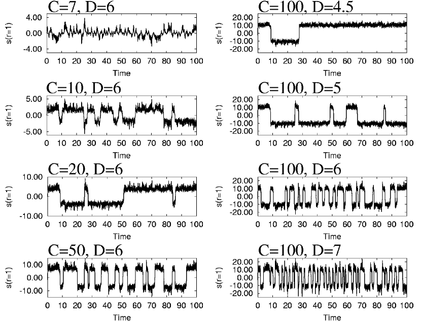
Figure 4: Time series for some selected values of $C$ and $D$.

II Numerical results.

We start with the noise-free case. Figure 1 shows the magnetic field evolution according to the equation system (2-4) for $D=0$ and different dynamo numbers $C$. The critical dynamo number is 6.78. The nearly harmonic oscillation for $C=6.8$ becomes more and more saw-tooth shaped for increasing $C$, with a pronounced asymmetry between the slow field decay and the fast field recreation during the reversal. At $C=7.24$ a transition to a steady dynamo has occurred.

In order to understand this behaviour, we examine in Fig. 2 the evolution of the magnetic field within approximately half a period of the anharmonic oscillation for the particular value $C=7.237$ at which the saw-tooth shape is already very pronounced. Figure 2a shows the time dependence of $s(r=1)$ during this half period, with the typical slow decay and the fast recreation of the field. This behaviour is analyzed in detail at 9 selected instants $\tau_{i}$ ($i=1...9$) for which the instantaneous fields $s(r,\tau_{i})$ (Fig. 2d) and the corresponding $\alpha(r,\tau_{i})$ (Fig. 2e, 2f) are depicted. The latter two plots reveal that $\alpha(r)$ undergoes only slight changes during the oscillation and that it comes very close to the unquenched, kinematic $\alpha_{kin}(r)$ (denoted by K) when the magnetic field is small in the middle of the reversal.

It is instructive to plug the instantaneous $\alpha(r,\tau_{i})$ profiles into an eigenvalue solver (for which the time derivatives on the left hand sides of Eqs. (2) and (3) are replaced by $\lambda s(r)$ and $\lambda t(r)$, respectively). Figure 2b and Fig. 2c show the resulting instantaneous growth rates and frequencies during the half-oscillation. Evidently, the reversal starts with a very slow field decay (slightly negative growth rate) which, however, accelerates itself and drives the system into an oscillatory behaviour (the frequency becomes different from zero for $2.0<\tau<4.5$). Around $\tau=4$, when the quenching of $\alpha$ is weak, the instantaneous growth rate reaches rather high values. Later we will see that for strongly supercritical dynamos these high growth rates result in a field dynamics that is much faster than what would be expected from the diffusion time scale.

In Figure 3a we relate this magnetic field evolution to the existence of exceptional points of the spectrum. It shows the instantaneous growth rate which results from the individual $\alpha(r,\tau_{i})$ profiles, and from the unquenched (kinematic) $\alpha(r)$ profile K. In addition to the growth rates at the actual dynamo number $C=7.237$ (indicated by the dashed vertical line), we have plotted the whole growth rate curves in the interval between $4.5<C<7.5$. At the exceptional point E_k of the kinematic $\alpha_{kin}(r)$, the first eigenvalue branch K1 coalesces with the second branch K2 and both continue as a pair of complex conjugate eigenvalues. For all other curves, only the exceptional point is indicated by $E_{i}$ whereas the branch of the second eigenvalue has been omitted. In this framework, a reversal can be described as follows: At the instant 1, the growth rate is located close to the maximum of the non-oscillatory branch which is slightly below zero. The resulting slow field decay accelerates itself, because the system moves down (instant 2) from the maximum of the real branch towards the exceptional point. Then the system enters the oscillatory branch (3-7). Finally the system moves back again (8,9) but with opposite polarity.

The transition point between oscillatory and steady dynamos ($C=7.239$) is characterized by the fact that the maximum of the non-oscillatory branch crosses the zero growth rate line. Beyond this point, the field is growing rather than decaying, leading to a stable fixed point somewhere to the left of the maximum of the non-oscillatory branch, and hence to a non-oscillatory dynamo (cf. the case $C=7.24$ in Fig. 1). If noise comes into play it will soften the sharp border between oscillatory and steady dynamos. This means, in particular, that even above the transition point, the noise can trigger a jump to the right of the maximum from were the described reversal process can start (Fig. 2).

Figure 5: Field intensity (virtual axial dipole moment) variations across five selected reversals, and their averages, computed for different values of $C$ and $D$. The time interval includes 80 kyr before (negative values) and 20 kyr after (positive values) a polarity transition. Note the quite different time scales for $C=8,D=1$ on one side, and for the other three examples on the other side.

Having identified the exceptional point and the nearby local maximum as the spectral features that are responsible for both the slow decay before and the fast recreation of the field after the polarity transition, one may ask now why the operator of the actual geodynamo should possess just such a special spectrum.

A preliminary answer to this question was given in EPSL and is illustrated in Fig. 3b. Roughly speaking, highly supercritical dynamos seem to have a tendency to saturate in a state for which the exceptional point and its associated local maximum lie close to the zero growth rate line. Interestingly, this happens independently on whether the exceptional point in the original kinematic case was above the zero growth rate line or below it. Our example with $\alpha_{kin}(r)=1.916\;C\;(1-6\;r^{2}+5\;r^{4})$ belongs to the second type. Starting from the kinematic $\alpha_{kin}(r)$, for which the exceptional point is well below the zero line, it rises rapidly above zero to a maximum value, but for even higher $C$ it moves back in direction to the zero line.

Without noise and for $C>7.239$, the position of the local maximum above the zero growth rate line leads to a steady dynamo. The presence of noise will sometimes bring the actual growth rate below zero, and then the indicated reversal process can start. A number of time series for different values of $C$ and $D$ is depicted in Fig. 4.

Figure 5 shows reversal details for four particular choices of $C$ and $D$. For later comparison with paleomagnetic data we have exhibited five typical reversals, and their averages, from 80 kyr before the polarity transition until 20 kyr after (except the case $C=8,D=1$ for which the reversal takes much longer).

III Comparison with paleomagnetic data.

In this section we will validate if our model can be fitted to real paleomagnetic data. For this purpose we have used recently published material about five reversals which occurred during the last two million years VALET2005 . Actually, the data shown in Fig. 6a have been extracted from Fig. 4 of VALET2005 . In all five curves, as well as in their averages, the asymmetry of the reversal process is clearly visible. The dominant features are a field decay over a period of 50-80 kyr and a rather sharp field recreation within 5-10 kyr. It has been an old-standing puzzle to explain in particular this fast recreation when a diffusive timescale of 200 kyr has to be taken into account. A possible solution of this problem is to assume a turbulent resistivity which is much larger than the molecular resistivity (e.g., by a factor 15-20 in HOYNG ).

The comparison of the real data with the numerically time series in Fig. 6b shows that this assumption of turbulent resistivity is by no means necessary. Apart from the slightly supercritical case $C=8,D=1$ which exhibits a much to slow magnetic field evolution, the other examples with $C=$20, 50, 100 and $D=6$ show very realistic time series with the typical slow decay and fast recreation. As noted above, the fast recreation results from the fact that in a small intervall during the transition the dynamo operates with an nearly unquenched $\alpha(r)$ profiles which yields, in case that the dynamo is strongly supercritical, rather high growth rates.

Figure 6: Comparison of paleomagnetic reversal data and numerically simulated ones. (a) Virtual axial dipole moment (VADM) during the 80 kyr preceeding and the 20 kyr following a polarity transition for five reversals from the last 2 million years (data extracted from VALET2005 ), and their average. (b) Comparison of the average curve of (a) with the four average curves of Fig. 5. The field scale for the numerical values has been fixed in such a way that the intensity in the non-reversing periods matches approximately the observed values.

IV Conclusions

Based on former results in PRL and EPSL , we have shown that a simple but strongly supercritical $\alpha^{2}$ dynamo model exhibits a number of features which are typical for Earth’s magnetic field reversals, in particular an asymmetric shape and correct timescales for the field decay and field recreation.

As it does not include the necessary North-South asymmetry of $\alpha$ we cannot claim that our model is an appropriate model of the geodynamo. However, recent papers by Giesecke et al. have shown that a) even in such realistic models $\alpha$ may exhibit a sign change along the radius GIES and b) that such models can also give rise to reversals GIESAN . Therefore, it seems worthwhile to identify the indicated reversal scenario in this and in more complicated geodynamo models.

References

- (1) J.-P. Valet and L. Meynadier. Geomagnetic field intensity and reversals during the past 4 million years. Nature, vol. 366 (1993), pp. 234–238.
- (2) J.-P. Valet, L. Meynadier, and Y. Guyodo. Geomagnetic dipole strength and reversal rate over the past two million years. Nature, vol. 435 (2005), pp. 802–805.
- (3) J. A. Tarduno, R. D. Cottrell, and A. V. Smirnov. High geomagnetic intensity during the mid-Cretaceous from Thellier analyses of single plagioclase crystals. Science, vol. 291 (2001), pp. 1779–1783.
- (4) M. Perrin and V. P. Shcherbakov. Paleointensity of the Earth’s magnetic field for the past 400 Ma: Evidence for a dipole structure during the mesozoic low. J. Geomagn. Geoelectr., vol. 49 (1997), pp. 601-614.
- (5) V. P. Shcherbakov, G. M. Solodovnikov, and N. K. Sycheva. Variations in the geomagnetic dipole during the past 400 million years (volcanic rocks). Izvestiya, Physics of the Solid Earth, vol. 38 (No. 2) (2002), pp. 113-119.
- (6) R. Heller, R. T. Merrill, and P. L. McFadden. The two states of paleomagnetic field intensities for the past 320 million years. Phys. Earth Planet. Inter., vol. 135 (2003), pp. 211–223.
- (7) A. Gailitis, O. Lielausis, E. Platacis, G. Gerbeth, and F. Stefani. Colloquium: Laboratory experiments on hydromagnetic dynamos. Rev. Mod. Phys., vol. 74 (2002), pp. 973–990.
- (8) T. Kato. Perturbation Theory of Linear Operators (Springer, Berlin, 1966).
- (9) F. Stefani and G. Gerbeth. Asymmetric polarity reversals, bimodal field distribution, and coherence resonance in a spherically symmetric mean-field dynamo model. Phys. Rev. Lett., vol. 94 (2005), Art. No. 184506; arxiv.org/physics/0411050
- (10) F. Stefani, G. Gerbeth, U. Günther, and M. Xu. Why dynamos are prone to reversals. Earth Planet. Sci. Lett., submitted (2005); arxiv.org/physics/0509118.
- (11) F. Krause and K.-H. Rädler. Mean-field Magnetohydrodynamics and Dynamo Theory (Akademie-Verlag, Berlin, 1980).
- (12) F. Stefani and G. Gerbeth. Oscillatory mean-field dynamos with a spherically symmetric, isotropic helical turbulence parameter . Phys. Rev. E, vol. 67 (2003); Art. No. 027302; astro-ph/0210412
- (13) P. Hoyng, D. Schmitt, M. A. J. H. Ossendrijver. A theoretical analysis of the observed variability of the geomagnetic dipole field. Phys. Earth Planet. Inter., vol. 130 (2002), pp. 143-157.
- (14) A. Giesecke, U. Ziegler, and G. Rüdiger. Geodynamo alpha-effect derived from box simulations of rotating magnetoconvection. Phys. Earth Planet. Inter., vol. 152 (2005), pp. 90-102.
- (15) A. Giesecke, G. Rüdiger, and D. Elstner. Oscillating -dynamos and the reversal phenomenon of the global geodynamo. Astron. Nachr., vol. 326 (2005), pp. 693–700.