Identification of nonlinear noisy dynamics of an ecosystem from observations of one of its trajectory components

Abstract

The problem of determining dynamical models and trajectories that describe observed time-series data (dynamical inference) allowing for the understanding, prediction and possibly control of complex systems in nature is one of very great interest in a wide variety of fields. Often, however, in multidimensional systems only part of the system’s dynamical variables can be measured. Furthermore, the measurements are usually corrupted by noise and the dynamics is complicated by an interplay of nonlinearity and random perturbations. The problem of dynamical inference in these general settings is challenging researchers for decades. We solve this problem by applying a path-integral approach to fluctuational dynamics Ludwig:75 ; Graham:77a ; Freidlin:84a ; Dykman:90 , and show that, given the measurements, the system trajectory can be obtained from the solution of the certain auxiliary Hamiltonian problem in which measured data act effectively as a control force driving the estimated trajectory toward the most probable that provides a minimum to certain mechanical action. The dependance of the minimum action on the model parameters determines the statistical distribution in the model space consistent with the measurements. We illustrate the efficiency of the approach by solving an intensively studied problem from the population dynamics of predator-prey system Hanski:01 where the prey populations may be observed while the predator populations or even their number is difficult or impossible to estimate. We emphasize that the predator-prey dynamics is fully nonlinear, perturbed stochastically by environmental factors and is not known beforehand (see e.g. Clark:03 ). No overall solution was previously available for this problem even in the deterministic case Kurths:04 ; Wood:01 . We apply our approach to recover both the unknown dynamics of predators and model parameters (including parameters that are traditionally very difficult to estimate) directly from measurements of the prey dynamics. We provide a comparison of our method with the Markov Chain Monte Carlo technique. As a further test of the method we demonstrate the reconstruction of the dynamics of chaotic Lorenz attractor driven by noise from measurements of only one if its trajectory component.

I Introduction

For quantitative understanding, predicting, and controlling time-varying phenomena it is necessary to relate observations to a mathematical model of a system dynamics. In a great number of important problems such model is multidimensional, nonlinear, stochastic and not known from “first principles”. Furthermore, often only part of the system’s variables can be measured and these measurements are corrupted by noise. The rest of the system variables are invisible, or hidden. In these settings, perhaps the most fundamentally difficult unsolved problem of dynamical inference is how and to which extent one can learn both the model parameters and system trajectory from a given set of incomplete trajectory measurements. A solution of this problem is of importance across many disciplines. Examples range from molecular motors Visscher:99 to coupled matter-radiation system Christensen:02 (see e.g.  Abarbanel:01 ; Kurths:04 ; Wood:01 ; Hanski:97 for further examples).

Here we present a solution to this problem using a path-integral approach to fluctuational dynamicsLudwig:75 . We show that, given the measurements, the most probable system trajectory can be obtained from finding the minimum of the mechanical action of a certain auxiliary Hamiltonian system under properly defined boundary conditions. The dependence of the minimum action on the system model parameters determines the statistical likelihood of different parametric models.

The method is used to solve an intensively studied problem from the population dynamics of the predator-prey systemHanski:97 ; Hanski:01 ; Turchin:00 where the cyclic dynamics of populations of small rodents is observed in Kilpisj$\ddot{a}$rvi, Finnish Lapland, 1952-1992 NERC (see Fig. 1(a)) while the number of predators is difficult or impossible to estimate. The predator-prey dynamics is fully nonlinear subject to seasonal and random perturbations. This is a classical longstanding problem in ecology Volterra:1926 and epidemiology (see e.g. Schwartz:84 ). In particular, the cited database accumulates nearly 5000 individual datasets with similar structure collected over more then 150 years of research. It is shown that the proposed approach allows to recover both the unknown dynamics of predators and model parameters directly from measurements of the prey dynamics.

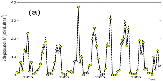
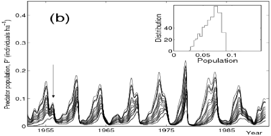
Figure 1: (a) Stochastic trajectory of the population dynamics of small rodents observed in Kilpisj$\ddot{a}$rvi, Finnish Lapland, 1952-1992 Hanski:97 is shown by yellow dots. Black solid line is shown to guide an eye. Dashed lines shows the solution of the optimization problem. (b) Black solid line shows recovered hidden dynamics of the population of the specialists predators obtained by varying parameters $r$ and $rK^{\prime}/K$ of the model (III). Parameters used to obtain these results are: r = 5.2 $\pm$ 2.5, rK’/K = -5.2 $\pm$ 2.5; s = 1.2; a = 15; g = 0.1; e1 = .8; e2 = .5; K = 90; Q = 30; $\sigma_{n}$ = 0.02; $\sigma_{p}$ = 0.02. The insert shows the cross-section of the weighted distribution of the dynamical trajectories for the year 1956 indicated by the arrow in the main figure.

II Path-integral approach to the problem of dynamical inference.

To formalize the discussion above note that in a typical experimental situation we observe $M$-dimensional time series of signals ${\cal Y}\equiv\{{\bf y}(t_{n})={\bf y}(t_{0}+hn),\,~{}n=\overline{0,{\cal K}}\}$, with the sampling step $h$. The unknown is the actual $L$-dimensional dynamical trajectory of the system ${\bf x}(t)$. We are interested in the case where $M\leq L$ so some of the trajectory components are hidden. Quantitative understanding of the time-varying phenomena underlying ${\cal Y}$ requires, in general, an expert input into the observed data in the form of a mathematical modelling framework for the system dynamics and for the measurement scheme. A commonly used dynamical and measurement equations for nonlinear models in the presence of random perturbations that apply to but by far not limited by the predator-prey ecological system described above are

$$\dot{x}_{i}(t)=K_{i}({\bf x}(t),{\bf c})+\xi_{i}(t),\quad\langle\xi_{i}(t)\,\xi_{j}(t^{\prime})\rangle=D_{ij}\delta(t-t^{\prime}),$$ (1)

$$y_{k}(t)=\sum_{i=1}^{L}B_{ki}\,x_{i}(t)+\beta_{k}(t),\quad\langle\beta_{k}(t)\,\beta_{l}(t^{\prime})\rangle=N_{kl}\,\delta(t-t^{\prime}).$$ (2)

Here we introduced continues-time interpolations $y_{k}(t)$ for components of the observed time-series ${\cal Y}$. This approximation can often be justified for a sufficiently small sampling interval $h$ and a large number of data points, ${\cal K}\gg 1$, in the time-series ${\cal Y}$. In (1) $x_{i}(t)$ ($i=1:L$) are dynamical variables composing a vector ${\bf x}(t)$ that describes an instantaneous state of the system. The system dynamics in (1) is governed by $L$-dimensional vector field with components $K_{i}$ depending on the set of parameters $\{c_{\alpha}\}\equiv{\bf c}$ and white Gaussian process with zero-mean components $\xi_{i}(t)$ characterized by a $L\times L$ correlation matrix $\hat{\bf D}$. The deterministic part of the measurement equation in (1) is described by $M\times L$ measurement matrix $\hat{\bf B}$ and the measurement error is described by the white Gaussian process with zero-mean components $\{\beta_{m}(t)\}$ and $M\times M$ measurement noise matrix $N_{n\,m}$ ($M\leq L$). Overall, the dynamical and measurement model (1) is characterized by the full set of the unknown parameters $\{{\cal M}_{\alpha}\}\equiv\{{\bf c},\hat{\bf B},{\bf\hat{D}},{\bf\hat{N}}\}$.

Due to the presence of dynamical and measurement noise the problem of dynamical inference must be cast in probabilistic terms. This can be done within a general framework of the Baeysian statistical approach  Congdon:01 ; Meyer:01 . A key statistical quantity is a so-called likelihood probability density functional (LPDF) ${\cal P}_{{\cal Y}}[{\bf x}(t);{\cal M}]$. It represents a joint probability density that the system trajectory is ${\bf x}(t)$ and the system parameter values are $\{{\cal M}_{\alpha}\}$ conditioned on the observed time-series ${\cal Y}$. We emphasize that in a real physical process the system has a distinct trajectory and parameter values. In this regard the LPDF represents a degree of uncertainty in our knowledge about these quantities obtained from the measurements and assuming some basic properties of the system fluctuational dynamics prior .

The explicit form of the LPDF can be obtained from (1) using the path-integral approach to fluctuational dynamics  Ludwig:75 ; Graham:77a ; Dykman:90 . We write ${\cal P}_{{\cal Y}}[{\bf x}(t);{\cal M}]=A_{{\cal Y}}\exp\left(-S_{{\cal Y}}[{\bf x}(t);\,{\cal M}]\right)$, where $A_{\cal Y}$ is a normalization constant and a negative log-likelihood functional $S_{\cal Y}$ is obtained in the Appendix A

$$S_{{\cal Y}}[{\bf x}(t);{\cal M}]=\frac{1}{2}\int_{0}^{T}dt\left[\left({\bf y}(t)-\hat{\bf B}\,{\bf x}(t)\right)^{T}{\bf\hat{N}}^{-1}\left({\bf y}(t)-\hat{\bf B}\,{\bf x}(t)\right)+{\bm{\nabla}}\cdot{\bf K}({\bf x}(t),{\bf c})\right.$$

$$\left.+\left(\dot{\bf x}(t)-{\bf K}({\bf x}(t),{\bf c})\right)^{T}\hat{\bf D}^{-1}(\dot{\bf x}(t)-{\bf K}({\bf x}(t),{\bf c}))\right]+\frac{{\cal K}}{2}\ln\left(\det(\hat{\bf D})\det(\hat{\bf N})\right).$$ (3)

Here $T={\cal K}h$ is a time length of the data record ${\cal Y}$. In what following we shall focus on the case $M<L$ that implies the existence of hidden variables. We note that despite hidden dynamical variables are not measured directly the functional $S_{\cal Y}$ (II) still depends on them explicitly because of the dynamic coupling between the variables imposed by the force field ${\bf K}$.

In many practically important cases available recording of a system trajectory, while containing only a part of dynamical variables, has sufficiently small time-step, long time duration and limited noise characteristics. Such measurements can provide a strong information that is sufficient to pin down both key model parameters of the system and its trajectory, or at least to extract strong correlations between them. In these cases the joint LPDF $P_{{\cal Y}}({\bf x}(t),{\cal M})$ will be well localized in the vicinity of one or more of its maxima where $\delta S/\delta{\bf x}(t)=0$ and $\{\partial S/\partial{\cal M}_{\alpha}=0\}$. In the case where a single maximum dominates LPDF its position corresponds to the trajectory ${\bf x}^{\rm opt}(t)$ and parameter values $\{{\cal M}_{\alpha}^{\rm opt}\}$ that the system most probably has, given the measurements ${\cal Y}$.

We now put forth a new paradigm in which a solution of the dynamical inference problem with hidden variables is obtained via the calculus of variations for the functional $S_{\cal Y}({\bf x}(t),{\cal M})$. The power of this approach is in its simplicity, efficiency and an insight that it provides to the solution of dynamical inference problem by drawing a close connection to the methods and concepts of classical mechanics, in particular, a least action principle.

We search for the minimum of $S_{\cal Y}({\bf x}(t),{\cal M})$ by alternatively computing the expected values of ${\bf x}(t)$ and model parameters in ${\cal M}$ from the solution of the two variational problems $\frac{\delta S}{\delta{\bf x}(t)}=0$ and $\frac{\delta S}{\delta{\cal M}}=0$. The first condition corresponds to a solution of the boundary value problem for an auxiliary mechanical system with the coordinate ${\bf x}$, momentum ${\bf p}$ and a Hamiltonian function $H({\bf x},{\bf p})$

$$H({\bf x},{\bf p})=-\frac{1}{2}\left({\bf y}-\hat{\bf B}\,{\bf x}\right)^{T}{\bf\hat{N}}^{-1}\left({\bf y}-\hat{\bf B}\,{\bf x}\right)-\frac{1}{2}\frac{\partial{\bf K}}{\partial{\bf x}}+{\bf K}{\bf p}+\frac{1}{2}{\bf p}^{T}\,\hat{\bf D}\,{\bf p},$$ (4)

$${\bf p}=\hat{\bf D}^{-1}(\dot{\bf x}(t)-{\bf K}).$$ (5)

We look for the solution of the Hamiltonian equations

$$\dot{\bf x}={\bf K}+\hat{\bf D}{\bf p},\qquad\dot{\bf p}=\frac{1}{2}\frac{\partial^{2}{\bf K}}{\partial{\bf x}^{2}}-\frac{\partial{\bf K}}{\partial{\bf x}}{\bf p}-\left({\bf y}-\hat{\bf B}\,{\bf x}\right)^{T}{\bf\hat{N}}^{-1}\hat{\bf B}$$ (6)

that satisfy the boundary conditions ${\bf p}(0)={\bf p}(t)=0$. If several solutions exist we choose the one providing a minimum of a functional $S_{{\cal Y}}[{\bf x}(t);{\cal M}]$ playing a role of a mechanical action. We then fix the inferred trajectory ${\bf x}(t)$ and update the value of the parameters in the set ${\cal M}$, using analytical solution of the second variational problem, $\frac{\delta S}{\delta{\cal M}}=0$, developed in our earlier research Smelyanskiy:05b (see Appendix A for details). This procedure is repeated iteratively until the desired convergence is achieved. The outcome of this algorithm is the most probable system trajectory ${\bf x}^{\rm opt}(t)$ and model parameters ${\cal M}^{\rm opt}$. The measure of their fitness to the observed data ${\cal Y}$ is $\propto\exp\left(S^{\rm opt}\right)$ where the globally minimum action $S^{\rm opt}=S_{{\cal Y}}[{\bf x}^{\rm opt}(t);\,{\cal M}^{\rm opt}]$.

The Bayesian approach for dynamical inference was initially proposed by Meyer and Christensenin Meyer:01 for the case where all variables were directly observed. The previous work on this subject (see e.g. Meyer:01 ; Rossi:02a ; Clark:03 ; Friedrich:03a ) was exclusively focusing on brute force numerical methods, such as Markov Chain Monte Carlo (MCMC). However our detailed study of MCMC approach for the problem of dynamical inference with hidden variables has shown that the functional $S_{{\cal Y}}({\bf x}(t),{\cal M})$ has multiple deep spurious minima in the space of piece-wise continuous trajectories $\{{\bf x}(t_{m});\,m=1:M\}$. These minima occur due to the contributions to the cost functions from the terms of the order of $\frac{(x_{i}(t_{k+1})-x_{i}(t_{k}))^{2}}{h^{2}}$. If one starts from a poor guess about both the system trajectory and model parameters MCMC search stacks in those minima and takes a prohibitively large time to converge (see Sec. V for details). In contrary, our approach avoids those spurious minima because the solution of the Hamiltonian boundary value problem (6) is achieved via large smooth variations in the space of continuous trajectories. This key finding reflects a basic property of a hidden-variable and parameter inference in a noisy dynamical system with continuous vector field ${\bf K}({\bf x},{\bf C})$: expected value of the inferred trajectory ${\bf x}^{\rm opt}(t)$ is a smoothly varying function of time whereas the measured signal ${\bf y}(t)$ is not.

We note that the likelihood distribution around the maximum is determined by the second variation $\delta^{2}S_{\cal Y}$ of the action with respect to the both ${\bf x}(t)$ and ${\cal M}$ computed at its minimum. In many cases, in particular in the case of a multi-modal LPDF, it is of interested to explicitly study the full shape of the LPDF in a reduced subspace of the model parameters while marginalizing the LPDF with respect to the other parameters and the system trajectory. Within our approach this can be handily done by computing the minimum action $S_{\rm opt}(c_{1},c_{2})$ using the above algorithm for different values of the parameters $(c_{1},c_{2})$.

However in many complex cases where observational and model errors are significant and hidden variables are present LPDF can have a very large number of local minima. In this case the more informative quantity is a distribution of local minima. To obtain it we pick at random some values of ($c_{1},c_{2})$ and converge to the nearest point ($c_{1}^{\prime},c_{2}^{\prime}$) of a local minimum of the action $S_{\rm opt}(c_{1},c_{2})$ where the conditions $\frac{\delta S}{\delta{\bf x}(t)}=0$ and $\frac{\delta S}{\delta{\cal M}}=0$ are satisfied. We then repeat this procedure many times for different starting values of ($c_{1}.c_{2})$. Then the histogram of the local minima ($c_{1}^{\prime},c_{2}^{\prime}$) weighed with the factors $\exp(-S_{\rm opt}(c_{1}^{\prime},c_{2}^{\prime})$ and appropriately normalized gives the distribution of local minima $P=P_{\cal Y}(c_{1},c_{2})$. We will demonstrate this approach in Sec. III for the inference of the population dynamics.

Finally, we emphasize that the prerequisite of the approach considered in this section is that LPDF computed at any set ${\cal M}$ of relevant parameter values has a sharp peak in the space of the system paths ${\bf x}(t)$ at some ${\bf x}^{\rm opt}(t)$ that depends on ${\cal M}$ (cf. Fig. 5).

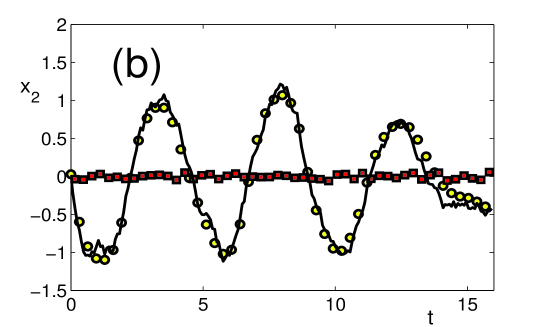
Figure 2: Result of the direct comparison of the path-integral and MCMC techniques for (a) observed variable $x_{1}(t)$ and (b) hidden variable $x_{2}(t)$. The actual dynamical trajectories $x_{1}(t)$ and $x_{2}(t)$ are shown by solid lines. The measured trajectory $y_{1}(t)$ is shown by dashed black line in figure (a) and is taken as initial guess for the solution $x_{1}(t)$. For an unobservable trajectory $x_{2}(t)$ initial guess is taken to be $y_{2}(t)=0$. The solution of the boundary value problem is shown by yellow circles. The MCMC solution is shown by red squares. The inset in the figure (a) shows the variation of the cost function as a function of time for MCMC algorithm (black dots) and for boundary value method (yellow circle).

III Inference of predator-prey model.

We now apply the method described above to reconstruction of the unknown predator dynamics and model parameters from the observed oscillations of small rodents in Finish Lapland. The observed time-series data is shown by yellow circles in the Fig. 1(a). To formulate the problem we first briefly summarize an expert input into observed data, see e.g.  Hanski:97 ; Turchin:00 ; Hanski:01 ; Hanski:03 for more details. It was argued Hanski:97 ; Hanski:01 that the most likely predators to potentially maintain oscillatory dynamics in rodent populations are small mustelids, weasels, and stoats which are notoriously difficult to observe and study in the field. It was further argued Hanski:97 ; Hanski:01 ; Hanski:03 that in addition to the dominating effect of these so-called specialist predators the population of rodents is strongly affected by generalists predators (such as foxes, owls and skua) and by seasonal (periodic) and stochastic variations of the environment. Based on these arguments the following equations were introduced to model observed ecological time series

$$\dot{N}=rN\left(1-e_{1}\sin(2\pi t)+\sigma_{n}\xi_{n}(t)\right)-(r/K)N^{2}-\frac{GN^{2}}{N^{2}+H^{2}}-\frac{CNP}{N+D},$$

$$\dot{P}=sP\left(1-e_{2}\sin(2\pi t)+\sigma_{p}\xi_{p}(t)\right)-sQ\frac{P^{2}}{N}.$$ (7)

Here the state of the system is characterized by the dynamical variables $N$ and $P$, corresponding to the density of rodents and predators, respectively. Taking into account a log-normal distribution of the measurement errors the measured rodent density $N^{\prime}$ is related to the actual (unknown) value $N$ via $N^{\prime}=N\exp(\sigma_{obs}\eta(t))$ where $\eta(t)$ is a white Gaussian noise of unit intensity. The predator density is not measured so the variable $P$ is hidden. In (III) $\{\xi_{n}(t),\xi_{p}(t)\}$ is a zero-mean white Gaussian vector of dynamical noise. The precise functional form is known neither for predation nor for numerical response of the predators and some modifications of the equations (III) where considered in the literature Turchin:00 .

The problem of dynamical inference is the following: Use 80 experimental points of corrupted by noise measurements to recover both hidden dynamics of predators $P=P(t)$ and the model of the nonlinear stochastic dynamics of small rodent in Fennoscandia represented by the full set of parameters from Eq. (III) and $\sigma_{osb}$. Since there were no general methods to recover neither hidden dynamics nor nonlinear models of stochastic systems it was always assumed (see e.g. Turchin:00 ; Hanski:01 ) that the goal to obtain solution of this problem is unrealistic and no attempt was made to solve it in the earlier research. Instead a number of models were developed Hanski:97 ; Turchin:00 ; Hanski:01 ; Hanski:03 from the first ecological principles and from the extensive field studies of the small rodents ecology. The outcome of the simulation of these models was compared to the experimental points to decide whether or not the model is capable of producing reasonable predictions. This approach although very valuable and often the only one available in practice has very limited statistical significance and can hardly be generalized.

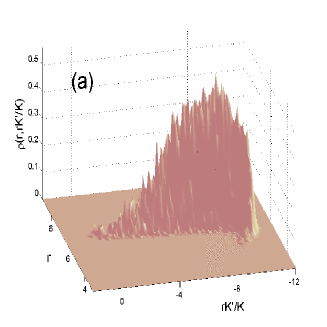
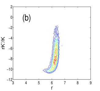
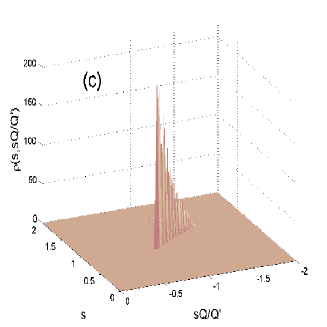
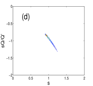
Figure 3: (a) Weighted distribution of the inferred values of the model parameters $r$ and $rK^{\prime}/K$. (b) The same distribution top view. (c) Weighted distribution of the inferred values of the model parameters $s$ and $sQ/Q^{\prime}$. (d) Top view of the same distribution.

The method introduced above provides a general and effective alternative approach to a solution of this ecological problem. First, we map the predator-pray model (III) directly onto the dynamical model with additive white noise considered in Eqs. (1) by making the change of variables: $x_{1}(t)=\log(N(t)/K^{\prime})$ and $x_{2}(t)=\log(Q^{\prime}P/K^{\prime})$ (here some known nominal values are used for the scaling coefficients $K^{\prime}$ and $Q^{\prime}$). Then the full set of unknown parameters ${\bf c}=\{r,s,e_{1},e_{2},K,G,C,Q,H,D,\sigma_{n},\sigma_{p},\sigma_{obs}\}$ and the trajectory of the predator density $P=P(t)$ is inferred from the observed data using the dynamical inference scheme described above (for the scaling of dynamical equations and precise ecological meaning of these parameters see Hanski:97 ; Hanski:01 ; Hanski:03 ). To present the solution of this inference problem we investigate the marginalized LPDF as a function of key model parameters that are notoriously difficult to estimate Hanski:97 using other techniques: carrying capacity $K$ and equilibrium ration between two populations $Q$ (see online supplement material for further details).

The results are shown in the Fig 1 and Fig. 3. It can be seen from the Fig 1 (a) that the model (III) can fit experimental data very well in a wide range of values of e.g. parameters $r$ and $rK^{\prime}/K$. This gives rise to a broad distribution of the possible dynamical trajectories of hidden predators shown in the Fig 1 (b). However, the likelihood functions of various trajectories are exponentially different. This fact is taken into account by weighting the corresponding distributions of the model parameters with the factor $\exp(-S_{\cal Y}\left[{\bf x}(t),{\bf c}\right])$. The weighted distributions of trajectories and model parameters is the main outcome of the statistical analysis of the ecological experimental data.

The weighted joint distributions of the inferred pairs of parameters ($r$, $r/K$) and ($s$, $sQ/Q^{\prime}$) are shown in the Fig. 3. Analysis of these distributions gives the following estimates of the model parameters $r=5.69\pm 0.49$, $rK^{\prime}/K=-6.0494\pm 1.25$, $K=76\pm 17$ $s=1.08\pm 0.31$, $sQ/Q^{\prime}=-1.17\pm 0.50$, $Q=43\pm 22$, $g=0.12\pm 0.3$, $a=13.2\pm 2.5$, $e_{1}=1.4\pm.4$, and $e_{2}=1\pm.5$ which are close to the values considered in the earlier ecological research Hanski:97 ; Turchin:00 ; Hanski:01 ; Hanski:03 . At the same time statistical analysis reveals that distributions for the parameters $\{H,D\}$ (in the range of values ???) are very flat and further information is needed for a more accurate estimate of their values.

IV Lemming oscillations in the high-arctic tundra in Greenland

The method can be further verified by analyzing experimental data obtained for the small rodents-predators community in high-arctic Greenland Hanski:03 . This data is very similar to the data collected in Fennoscandia with a important exception, namely, dynamics of both populations prey and predator was recorded very carefully in Greenland. Therefore, it has become possible to check if the predator dynamics reconstructed from the prey population alone coincides with the actual observations of the predator time series.

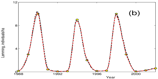
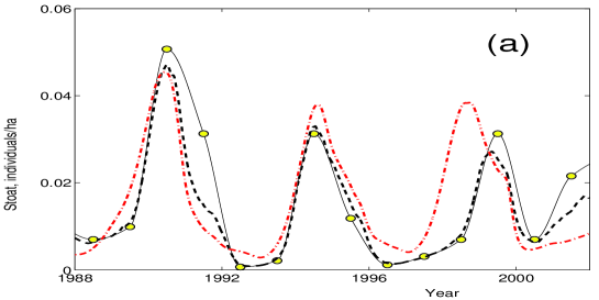
Figure 4: Lemming (a) and (b) stoat population (individuals/ha) observed in the high-arctic tundra in 1988–2002 Hanski:03 are shown by yellow circles. The thing solid line is shown to guide the eye. Dashed black lines show population dynamics inferred using model (IV) under assumption that the dynamics of both populations was measured in the experiment with measurement error 0.2. Dashdot lines show population dynamics inferred using model (IV) under assumption that only the dynamics of prey populations was measured in the experiment with measurement error 0.2 and the predator dynamics is hidden.

The experimental data (see Fig. 3) for the population oscillation in the lemming-stoat predator prey community were collected in the high-Arctic tundra in Greenland in 1988–2002 Hanski:03 . The time-variation of the predator and prey oscillations are also influenced by a number of generalists predators such as arctic fox, snowy owl, and long-tailed skua. We note that a very detailed model with experimentally measured numerical responses of various predators is available Hanski:03 to simulate this data. However, to analyze hidden predator population along the lines outlined in the previous section we notice that the organization of the lemming-stoat community in the high-arctic Greenland is very similar to the vole-weasel community in Finnish Lapland. So we attempt to fit the lemming-stoat population oscillations using the model (III) developed for the latter community Hanski:97 ; Turchin:00 ; Hanski:01 .

In this model the populations are scaled as $x=log(N/K^{\prime})$ and $y=log(\frac{Q^{\prime}P}{K^{\prime}})$ with some assumed values of the carrying capacity $K^{\prime}$ and proportionality constant $Q^{\prime}$ ($K^{\prime}$ and $Q^{\prime}$ are known, while actual values $K$ and $Q$ are not known and have to be inferred). The time-variations of $x(t)$ and $y(t)$ are described by the following set of equations Hanski:97

$$\dot{x}=r\left(1-e_{1}\sin(2\pi t)\right)-r\frac{K^{\prime}}{K}e^{x}-g\frac{e^{x}}{e^{2x}+h^{2}}-a\frac{e^{x}}{e^{2}+d},+D_{n}\xi_{n}(t)$$

$$\dot{y}=s\left(1-e_{2}\sin(2\pi t)\right)-s\frac{Q}{Q^{\prime}}e^{y-x}+D_{p}\xi_{p}(t).$$ (8)

The parameters of these equations have the following Hanski:97 meaning. The vole population is characterized by: (i) the intrinsic rate of the vole population growth $r$ with possible values in the range: 4 - 7 yr^-1; (ii) the dimensionless amplitude of seasonal forcing $e$ with range: 0.5 - 1; (iii) prey carrying capacity $K$ with range: 100 - 300 voles ha^-1. The specialist predator population is described by: (i) intrinsic rate of weasel population growth $s$ with range: 1- 1.5 yr^-1; (ii) minimum consumption per predator $C$ with range: 500-700 voles yr^-1 weasel^-1; (iii) half saturation constant $D$ with range: 5-6 voles ha^-1; (iv) predator-prey constant ratio $Q$ with range: 20-40 voles weasel^-1. The generalist predation is characterized by: (i) the maximum rate of mortality $G$ with range: 70 - 125 voles ha^-1 yr^-1 and (ii) half-saturation prey density $H$ with range: 11-16 voles ha^-1.

First, we try to fit this model to the experimental data taking into account measurements of both populations. To avoid the problem related to the fact that continuous model is being fitted to the experimental points measured only once a year we interpolate experimental points for predator and prey using a piecewise cubic Hermite interpolation with time step $h=0.001$ year. The corresponding results of the fit are shown by the dashed black line in the Fig. 4(a) and (b). We note that the model (IV) can fit very well experimental data. However, this agreement has a limited statistical significance since we are fitting 30 experimental points by a nonlinear model with 18 parameters. It turns out that the same experimental data can be well fit in a broad range of the values of the model parameters. A detailed study of the landscape of the log-likelihood function is needed to choose the most probable model. We defer this study to a future publication. In the present study our main goal is to verify that even in the absence of the measurements of the predator population we can still recover both hidden dynamics of the predator and the model parameters although with degraded accuracy.

Table 1: Inference results for the parameters of the model (IV) obtained by two methods: Value I were obtained assuming that both populations (lemming and stoat) were measured; Value II were obtained assuming that only lemming population were measured. Experimental points in both cases were interpolated using piecewise cubic Hermite interpolation with time step $h=0.001$ year.

Parameter	Value I		Value II
$r$	$2$.	$24$	$4$.	$53$
$s$	$0$.	$76$	$0$.	$99$
$rK^{\prime}/K$	$-4$.	$07$	$-7$.	$26$
$a$	$-7$.	$96$	$-14$.	$18$
$g$	$0$.	$41$	$0$.	$39$
$sQ/Q^{\prime}$	$-0$.	$82$	$-0$.	$95$
$e_{11}$	$0$.	$63$	$0$.	$35$
$e_{21}$	$0$.	$32$	$0$.	$09$
$e_{12}$	$0$.	$28$	$0$.	$40$
$e_{22}$	$-0$.	$21$	$-0$.	$29$

To this end we now infer both hidden dynamics of the stoat population and the model parameters assuming that only population of lemming was measured. The corresponding inference results are shown in the Fig. 4(a) and (b) by the red dash-dot lines. The values of the parameters inferred in both cases are summarized in the Table 1.

We conclude that even in the case of incomplete corrupted by noise measurements of the population dynamics our method allows one to recover both hidden dynamics of invisible predator and the model parameters.

IV.1 3D distribution of the predator trajectories

Finally we analyze a distribution of the most probable predator trajectories for different model parameter values taken at multiple minima of LPDF discussed above (see Fig. 3). We search for local minima of LPDF with respect to the set of coefficients ${\cal M}=\{r,rK^{\prime}/K,s,sQ/Q^{\prime}\}$ in the region $\{5.2000\pm 4,-5.2000\pm 4,1.2000\pm 1.1,-1.2000\pm 1.1\}$. At each local minima ${\cal M^{\prime}}$ we find the most probable predator trajectory ${\bf x}_{\rm opt}(t)$ by solving a boundary value problem described above and attach the statistical weight to this trajectory $\propto\exp(-S({\bf x}_{\rm opt}(t),{\cal M^{\prime}})$. The resulting 3D distribution of the weighted predator trajectories is shown in the Fig 5.

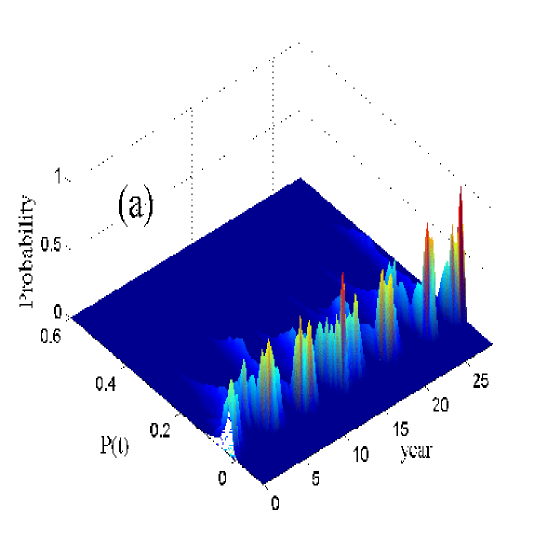
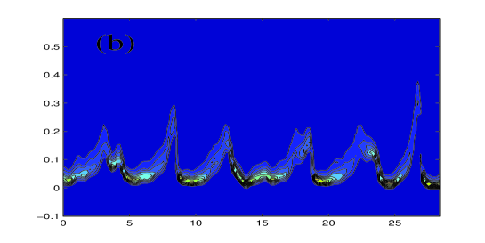
Figure 5: (a) probaility distribution of the predator trajectories at local minima of LPDF; (b) the corresponding contour plot. Local minima of LPDF with respect to four model parameters were sampled in the region: $r=\{5.2000\pm 4,rK^{\prime}/K=-5.2000\pm 4,s=1.2000\pm 1.1,sQ/Q^{\prime}=-1.2000\pm 1.1\}$. Other parameters in this test were: $C/Q^{\prime}=20.9223$, $G/K^{\prime}=0.2401$, $re_{1}=2.2493$, $se_{2}=0.5027$, $(H/K^{\prime})^{2}=0.04$, $D/K^{\prime}=0.04$.

V Comparison of path-integral based inference with Markov Chain Monte Carlo method

To compare directly the results of the reconstruction obtained by the path-integral method and by MC algorithm we simplify problem and consider oscillations in a two-dimensional system of the form

$$\begin{array}[]{ll}&\dot{x}_{1}=1.5x_{2}+x_{1}^{2}x_{2}-0.2x_{1}^{3}+\sqrt{D_{11}}\xi_{1}(t),\\ &\dot{x}_{2}=-x_{1}+\epsilon(1-x_{1}^{2})x_{2}+\sqrt{D_{22}}\xi_{2}(t),\\ \end{array}$$ (11)

where $\epsilon=0.1$ and $D_{11}=D_{22}=0.04$. We assume that only $x_{1}(t)$ is measured with measurement noise $\eta(t)$ of intensity $N=0.2$ to produce an observed time series

$$y_{1}(t)=x_{1}(t)+\sqrt{N}\eta(t),$$

while the second variable is missing.

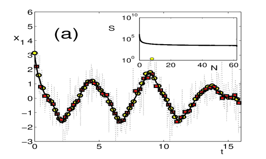
Figure 6: Result of the direct comparison of the path-integral and MCMC techniques for (a) observed variable $x_{1}(t)$ and (b) hidden variable $x_{2}(t)$. The actual dynamical trajectories $x_{1}(t)$ and $x_{2}(t)$ are shown by solid lines. The measured trajectory $y_{1}(t)$ is shown by dashed black line in figure (a) and is taken as initial guess for the solution $x_{1}(t)$. For an unobservable trajectory $x_{2}(t)$ initial guess is taken to be $y_{2}(t)=0$. The solution of the boundary value problem is shown by yellow circles. The MCMC solution is shown by red squares. The inset in the figure (a) shows the variation of the cost function as a function of time for MCMC algorithm (black dots) and for boundary value method (yellow circle).

We find maximum of the posterior PDF $p_{\rm ps}({\bf x},{\cal M}|{\bf y})$ in the space of dynamical trajectories $\{{\bf x}(t)\}$ by applying two methods: path-integral approach as described above and Markov Chain Mote Carlo (MCMC) using Metropolis-Hastings algorithm within Gibbs sampling scheme (see e.g. Ruanaidh:96 ). The results are shown in the Fig. 4. It can be seen from the figure that the MCMC algorithm can indeed be used to reconstruct dynamical trajectory from the noisy measurements. However, in the case of missing variable the MCMC fails to recover correct solution. The reason is that the later requires large smooth variations of the trajectory, while the MCMC algorithm is searching in the space of discontinuous nondifferentiable trajectories and as a result converges to multiple deep spurious minima produced by the terms of the order $\frac{(x_{k+1}-x_{k})^{2}}{h^{2}}$ in the cost function (II). Similar problem appears already in deterministic case Kurths:04 , where the multiple shooting technique is applied to solve the problem. We note that our approach is more general. It is valid both in stochastic and deterministic case and avoids logistic and technical problems related to dividing trajectory on arbitrary number of piece-wise continuous solutions and on gluing these solution together.

V.1 Lorenz attarctor

WE found our method to be sufficiently robust to work in the case of more then one hidden variable. To demonstrate this we consider the archetypical chaotic nonlinear system of Lorenz,

$$\begin{array}[]{rcl}{\dot{x}}_{1}&=&\sigma\,(x_{2}-x_{1})+\xi_{1}(t),\\ {\dot{x}}_{2}&=&r\,x_{1}-x_{2}-x_{1}\,x_{3}+\xi_{2}(t),\\ {\dot{x}}_{3}&=&x_{1}\,x_{2}-b\,x_{3}+\xi_{3}(t),\end{array}$$ (12)

driven by zero-mean white Gaussian noise processes $\xi_{l}(t)$ with covariance $\langle\xi_{l}(t)\,\xi_{l^{\prime}}(t^{\prime})\rangle=D_{ll^{\prime}}\,\delta(t-t^{\prime})$. Synthetic data (with no measurement noise) were generated by simulating (12) using the standard parameter set $\sigma=10$, $r=28$, $b=\frac{8}{3}$, and for various levels of dynamical noise intensities. It is assumed that the trajectory component $x(t)$ shown in Fig. 7(a) is measured directly (no measurement noise) while the components $y(t)$ and $z(t)$ are not observed (hidden variables). The results of the trajectory inference are shown in Fig. 7(b,c,d).

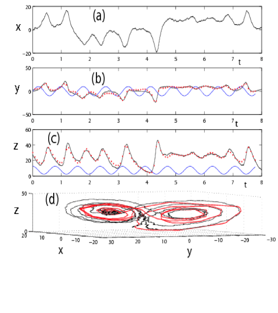
Figure 7: (a) Measured variable $x(t)$ for the following system parameters: $D_{11}=2.5$, $D_{22}=3.0$, and $D_{33}=3.5$, $r=28$, $\sigma=10$, $b=8/3$. (b) and (c) Actual values of the unknown dynamical variables $y(t)$ and $z(t)$ are shown by the black line. Inferred values are shown by the red dots. (d) Actual trajectory of the system in 3D space of the variables $x,y,z$ (black solid line) is compared with the inferred trajectory (red line).

VI Conclusions

Is has been assumed up to now that a lack of observational data for predator populations constituted a fundamental obstacle to the inference of ecological parameters from experimental data Hanski:97 ; Turchin:00 ; Hanski:01 ; Hanski:03 . A conclusion that can be drawn from the above results that this is not necessarily the case. Using the methods described above it is possible to reconstruct both invisible dynamics of predators population and the model parameters directly from measurements of prey populations, even those containing some measurement errors and uncertainties.

Note, that much of the studies across many scientific disciplines rely on the analysis of the extremal properties of the effective action similar to (II) in various function spaces (cf. e.g. Borland:92a ; Borland:96 ; Luchinsky:97c ; Smelyanskiy:97a ; Luchinsky:02b ; Smelyanskiy:05b ). For example, solution of the problems of large occasional deviations in noisy dynamical systems is given by the minimum of the functional (II) with no measurement term. Unlike the dynamical inference searching for the trajectory and model parameters that the system has with high probability, the theory of large deviations is concerned with an optimal fluctuation, or a least improbable path of the system to reach a remote state from the attractor during the rare event. However the solution of both problems provides a global minimum to the functional (II) in the space of dynamical trajectories and is equivalent to a certain Hamiltonian dynamics in an extended phase space. In the theory of large deviations the corresponding Hamiltonian is called Wentzel-Friedlin Hamiltonian Freidlin:84a . The dynamical quantities appearing within this Hamiltonian theory have precise physical meaning and are accessible for direct experimental measurements Luchinsky:97c ; Dykman:00a ; Luchinsky:02b . Very similar optimization problems also occur in the context of stochastic optimal control of large deviations  Freidlin:70b ; Smelyanskiy:97a ; Luchinsky:02b and the related Hamiltonian can sometimes be identified Luchinsky:02b with so-called Pontryagin Hamiltonian Hagedorn:82 playing a key role in the theory of optimal control. We note however that the dynamical inference Hamiltonian $H_{\cal Y}({\bf x},{\bf p})$ (4) is of a qualitatively new type. It depends explicitly on the time-varying measurement signal ${\bf y}(t)$ that plays a role of a ’control force’ in the Hamiltonian dynamics. These considerations suggest that the proposed path-integral approach to the problem of dynamical inference with hidden variables is a general one and sets the solution of this problem into the standard mathematical context. It is valid both in deterministic and stochastic case and is a natural generalization of the earlier ad hoc approach to the dynamical inference of deterministic systems Domselaar:75 ; Kurths:04 .

We believe that methods of Hamiltonian theory will provide a new topological insight to the solutions of complex problems of a dynamical inference with hidden variables. For example, in many cases the observed data are not sufficient to discriminate with high probability between the different values of system parameters and/or the forms of its hidden trajectory component. This corresponds to a certain ’degeneracy’ set in the joint functional space $({\bf x}(t),{\cal M})$ where the functional $S$ takes a constant maximum value. In general, the degeneracy set will be determined by the properties of the corresponding Lagrangian manifold associated with the auxiliary Hamiltonian system (4) and conditions ${\bf p}(0)={\bf p}(T)=0$. We also note that whenever the dynamical inference converges to a right solution the inferred system trajectory and parameter values correspond to a sufficiently small momentum $|{\bf p}(t)|$ (of the order of noise intensities, $D,\,N$) and the minimum action $S^{\rm opt}\sim 1$. However in certain cases the global minimum of $S$ corresponds to a much larger momentum $|{\bf p}(t)|\gg N,\,D$ and $S^{\rm opt}\gg 1$. Then the fitness to the data ${\cal Y}$ is poor for any choice of parameters and trajectory. This implies that model assumptions (1) do not capture some important properties of the real-world system (a so called, “model error”). Overall, the locations of maxima of effective action $S$ dominating the LPDF, their relative weights, as well as the topological structure in the joint functional space $({\bf x}(t),{\cal M})$ answer the statistical question of what can or cannot be learned with a high likelihood about the system at hand given the available data and basic assumptions about the dynamical model.

Our results also reveal a remarkable property of the dynamical inference with incomplete measurements. In the absence of the model error the system parameters can be learned with uncertainties $\langle(\delta M_{\alpha})^{2}\rangle$ that are not limited by the dynamical nor measurement noise intensities. In particular, $\langle(\delta M_{\alpha})^{2}\rangle\lesssim 1/T$, for large $T$ (see Appendix for the details of the derivation). On the other hand, the uncertainty in the inferred system trajectory $\langle(\delta x_{j}(t))^{2}\rangle$ is bounded from below by the dynamical and measurement noise. This effect can appear counterintuitive to a reader, because hidden variables and model parameters are trading against each other in the log-likelihood (II) that could seemingly cause the parameter and trajectory errors to be comparable with each other. The explanation for the above effect is that the trajectory points ${\bf x}(t_{m})$ at closely spaced instances of time $t_{m}$ are correlated with each other, those correlations are being extracted and accumulated during the dynamical inference which we presented in the paper and this leads to the shrinking of the parameter error with time below the noise level.

The proposed method should be applicable to a broad range of problems in science and technology ranging from extracting parameters of molecular motors from the measurements of their progression along microtubules Visscher:99 ; Kawaguchi:01 to the inference of a climate forcing mechanisms from reconstructed from the measurements of carbon dioxide in ocean sediment Rahmstorf:02 . We also expect this method to be particularly useful in the context of physiological measurements where it is especially important to relate difficult-to-access parameters to noninvasively-measured data Seidel:95 ; Seidel:98a . The open question to be addressed in the near future is an extension of this theory to quantum and spatially extended systems.

APPENDIX: BAYESIAN INFERENCE OF CONTINUOUS NOISE-DRIVEN DYNAMICAL SYSTEMS FROM INCOMPLETE MEASUREMENTS

Within the Bayesian framework the problem of dynamical inference is to determine the conditional probability density functional (PDF) defined over the set of the unknown quantities $(\bf x(t),{\cal M})$, subject to observations ${\bf y}(t)$. The later, so-called posterior PDF, $p_{\rm{ps}}[{\bf x}(t);{\cal M}|\,{\bf y}(t)]$ is found using Bayes’ theorem

$$p_{\rm{ps}}[{\bf x}(t);{\cal M}|\,{\cal Y}]\propto\,p_{\rm ob}[{\bf y}(t)\,|\,{\bf x}(t),{\cal M}]\,p_{\rm{pr}}[{\bf x}(t),{\cal M}].$$ (13)

Here the missing proportionality coefficient is simply a normalization factor. $p_{\rm{pr}}[{\bf x}(t),{\cal M}]$ is a so-called prior PDF that provides the joint statistical information about ${\bf x}(t)$ and ${\cal M}$ before the measurements ${\bf y}(t)$ were made. The prior PDF can be written in the form: $p_{\rm{pr}}[{\bf x}(t),{\cal M}]={\cal P}[{\bf x}(t)|\,{\cal M}]\,p_{0}({\cal M})$. Here $p_{0}({\cal M})$ is some prior distribution of model parameters and ${\cal P}[{\bf x}(t)|\,{\cal M}]$ is the PDF of finding a realization of the dynamical trajectory ${\bf x}(t)$ for a given set of the system parameters ${\cal M}$  Ludwig:75 ; Graham:77a ; Dykman:90 . This functional directly depends on the form of the stochastic dynamical model (1) and its parametrization. For example, in the case of the additive white noise considered in (1) this functional has the form  Ludwig:75 ; Graham:77a

$${\cal P}[{\bf x}(t)|\,{\cal M}] \propto \left(\left(\frac{2\pi}{h}\right)^{L}{\rm det}\hat{\bf D}\right)^{-{\cal K}/2}\,$$ (15)

$$\times\,\exp\left[-\frac{1}{2}\int_{0}^{T}dt\left({\bm{\nabla}}\cdot{\bf K}+(\dot{\bf x}-{\bf K}^{T})\hat{\bf D}^{-1}(\dot{\bf x}-{\bf K})\right)\right],$$

where ${\bf x}\equiv{\bf x}(t)$, ${\bf K}\equiv{\bf K}({\bf x}(t),{\bf C})$ and a coefficient of proportionality is a normalization factor.

In Eq.(13) $p_{\rm ob}[{\cal Y}|{\bf x}(t),{\cal M}]$ is a conditional PDF to observe the measurement signal ${\bf y}(t)$ for a specific realization of a system trajectory ${\bf x}(t)$ and model parameters ${\cal M}$. For the continuous-time measurement model considered in (1) this PDF takes the form

$$p_{\rm ob}[{\cal Y}\,|{\bf x}(t),{\cal M}] = \left(\left(\frac{2\pi}{h}\right)^{M}{\rm det}\hat{\bf N}\right)^{-{\cal K}/2}\,$$

$$\times\,\exp\left[-\frac{1}{2}\int_{0}^{T}dt\,\left({\bf y}(t)-\hat{\bf B}\,{\bf x}(t)\right)^{T}{\hat{\bf N}}^{-1}\left({\bf y}(t)-\hat{\bf B}\,{\bf x}(t)\right)\right],$$

and describes the zero-mean Gaussian statistics of the measurement error ${\bm{\beta}}(t)={\bf y}(t)-\hat{\bf B}\,{\bf x}(t)$. Returning back to the original discreet-time measurements ${\cal Y}=\{{\bf y}(t_{m}),\,t_{m}=m\,h,\,m=1:{\cal K}\}$ one gets $\langle\beta_{k}(t_{m})\beta_{k^{\prime}}(t_{m}^{\prime})\rangle=N_{kk^{\prime}}/h\,\delta_{mm^{\prime}}$.

Prior PDF $p_{0}[{\cal M}]$ usually represents a posterior PDF obtained as a result of the dynamical inference based on the previous sets of data and on the expert knowledge about possible domains for the system parameters. Often the inference is entirely based on the present set of data and the prior PDF is assumed to be completely uniform. In this case the posterior PDF $p_{\rm{ps}}[{\bf x}(t);{\cal M}|\,{\cal Y}]$ in (13) is usually referred to as a likelihood PDF. We denote the later as $p_{{\cal Y}}[{\bf x}(t);{\cal M}]$ and obtain:

$$p_{{\cal Y}}[\,{\bf x}(t);{\cal M}]\propto p_{\rm ob}[{\cal Y}\,|{\bf x}(t),{\cal M}]\,{\cal P}[{\bf x}(t)|\,{\cal M}].$$ (17)

Using Eqs. (15) and (APPENDIX: BAYESIAN INFERENCE OF CONTINUOUS NOISE-DRIVEN DYNAMICAL SYSTEMS FROM INCOMPLETE MEASUREMENTS) in (17) one can rewrite the likelihood PDF in the form

$$p_{{\cal Y}}[{\bf x}(t);{\cal M}]=A_{\cal Y}\,\exp\left(-S_{\cal Y}[{\bf x}(t);{\cal M}]\right).$$ (18)

where the negative log-likelihood function $S_{\cal Y}$ is given in (II) and $A_{\cal Y}$ is a normalization factor that does not depend on ${\bf x}(t)$ nor ${\cal M}$.

Calculation of the expectation values using the maximum-likelihood estimation.

In the asymptotic limit of a sufficiently long and dense data record ${\cal Y}$ and low noise intensities the PDF $p_{{\cal Y}}[\,{\bf x}(t);{\cal M}]$ is, generally, a very steep function of its arguments and the derivatives of $S_{\cal Y}$ with respect to ${\bf x}(t)$ and ${\cal M}$ are much greater then 1 (assuming all quantities are dimensionless). In this case the expectation values of the system trajectory $\langle{\bf x}(t)\rangle$ and the model parameters $\{\langle{\cal M}_{\alpha}\rangle\}$ for a given measurement record ${\cal Y}$ can be obtained by computing a maximum of the likelihood PDF in the joint space $(\bf x(t);{\cal M})$. The conditions for the maximum have the form of the variational equations

$$\frac{\delta S_{\cal Y}}{\delta{\bf x}(t)}=0,\\$$ (19)

that have to be solved simultaneously with the system of the algebraic equations

$$\frac{\partial S_{\cal Y}}{\partial{\bf c}}=0,$$ (20)

$$\frac{\partial S_{\cal Y}}{\partial\hat{\bf D}}=0,\qquad\hat{\bf D}=\hat{\bf D}^{T},$$ (21)

$$\frac{\partial S_{\cal Y}}{\partial\hat{\bf N}}=0,\qquad{\bf N}={\bf N}^{T},$$ (22)

$$\frac{\partial S_{\cal Y}}{\partial\hat{\bf B}}=0.$$ (23)

Eqs.(19) for the minimum of the action $S_{\cal Y}$ with respect to the trajectory components $x_{i}(t)$ correspond to the Hamiltonian equations (4),(6) with the appropriate boundary conditions described in the main text.

Inference of the model parameters was considered in Smelyanskiy:05b under the simplifying assumptions that the measurement noise is zero, there are no hidden variables and the force field is linear in the parameters $\{c_{\alpha}\}$ (but generally, nonlinear in ${\bf x}$). Below we provide the generalization of the results of the Ref. Smelyanskiy:05b that allows us to infer the unknown parameters of the measurement model and does not relay on the linearity of ${\bf K}$ in ${\bf c}$.

The Eq. (20) gives the conditions of the minimum of $S_{\cal Y}$ with respect to the parameters $\{c_{\alpha}\}$ of the force field ${\bf K}({\bf x}(t),{\bf c})$. Using the Eq. (II) we obtain these conditions in the following form:

$$\int_{0}^{T}dt\,\frac{\partial{\bf K}}{\partial c_{\alpha}}\,\hat{\bf D}^{-1}\,[\dot{\bf x}(t)-{\bf K}({\bf x}(t),{\bf c})]=\frac{1}{2}\int_{0}^{T}dt\frac{\partial}{\partial c_{j}}\,{\bm{\nabla}}\cdot{\bf K}({\bf x}(t),{\bf c}).$$ (24)

Solving the Eqs. (21) and (22) with respect to $\hat{\bf D}$ and $\hat{\bf N}$, respectively, we obtain

$$D_{ij} = \frac{1}{{\cal K}}\int_{0}^{T}dt\,[\dot{x}_{i}-K_{i}({\bf x}(t),{\bf c})]\,[\dot{x}_{j}-K_{j}({\bf x}(t),{\bf c})],$$ (25)

$$N_{kl} = \frac{1}{{\cal K}}\int_{0}^{T}dt\,[\dot{y}_{k}(t)-\sum_{i=1}^{L}B_{ki}x_{i}(t)]\,[y_{l}(t)-\sum_{j=1}^{L}B_{lj}x_{j}(t)].$$ (26)

Finally, the Eq. (23) can be re-written in the explicit form of the system of linear equations for the matrix elements of $\hat{\bf B}$

$$\sum_{k,i}\Lambda_{ki}^{k^{\prime}i^{\prime}}\,B_{k^{\prime}i^{\prime}}=W_{ki},$$ (27)

where

$$\Lambda_{ki}^{k^{\prime}i^{\prime}}=(\hat{\bf N}^{-1})_{kk^{\prime}}\,\int_{0}^{T}dt\,x_{i^{\prime}}(t)\,x_{i}(t),$$ (28)

$$W_{ki}=\sum_{l}(\hat{\bf N}^{-1})_{kl}\int_{0}^{T}dt\,y_{l}(t)\,x_{i}(t).$$ (29)

One solves simultaneously Eqs. (24)-(29) and the Hamiltonian equations (4),(6) and selects the solution with the minimum value of $S_{\cal Y}$.

Calculation of the variances.

We now consider how the variances of the model parameters around the maximum of the LPDF depend on the noise intensity and length of the observation record. We focus on demonstrating of the main effect mentioned in Conclusion and for brevity we assume that there are two dynamical variables, one of them, $x_{1}$, is hidden, and the other, $x_{2}$, is observed with zero measurement error, $x_{2}(t)=y_{2}(t)$. We assume that the correlation matrix $\hat{\bf D}$ of the dynamical noise is diagonal with the small nonzero matrix elements $D_{j}\equiv D_{jj}\ll 1$. We also assume that there is only one unknown model parameter $c$ and it enters the expression for the vectorial force field ${\bf K}={\bf K}({\bf x},c)$.

The action functional in the reduced space $S_{{\cal Y}}[x_{1}(t),y_{2}(t);c]\equiv s[x_{1}(t);c]$ has the form

$$s[x_{1}(t);c] = \frac{1}{D_{1}}\int_{0}^{T}dt\,\left[\frac{1}{2}(\dot{x}_{1}(t)-\bar{K}_{1}(x_{1}(t),y_{2}(t);c))^{2}-V(x_{1}(t),t,c)\right]$$ (30)

$$V(x_{1},t,c) \equiv -\frac{D_{1}}{2D_{2}}(\dot{y}_{2}(t)-K_{2}(x_{1},y_{2}(t);c))-\frac{D_{1}}{2}\,\sum_{j=1}^{2}\frac{\partial K_{j}(x_{1},y_{2}(t);c)}{\partial x_{j}}.$$ (31)

At certain point $(x_{1}^{\rm opt}(t),c^{\rm opt})$ where the action $s[x_{1}(t),c]$ reaches its minimum the conditions $\delta s/\delta x_{1}(t)=0$ and $\partial s/\partial c=0$ are satisfied. Consider now the trajectory $x_{1}=x(t,c)$ corresponding to the partial minimum of the action with respect to $x_{1}(t)$ with the value of the model parameter fixed: $\min_{x_{1}(t)}s[x_{1}(t),c]=s[x(t,c),c]$. The Hamiltonian equations (6) for $x(t,c)$ have the following form:

$$\dot{x}_{1} = p_{1}+K_{1}(x_{1}(t),y_{2}(t);c),$$ (32)

$$\dot{p}_{1} = -p_{1}\frac{\partial K_{1}(x_{1}(t),y_{2}(t);c)}{\partial x_{1}}-\frac{\partial V(x_{1}(t),t;c)}{\partial x_{1}},\quad p_{1}(0)=p_{1}(T)=0.$$ (33)

Of central interest for us here is the coefficient of expansion of the action $s[x(t,c);c]$ in $c-c^{\rm opt}$

$$s[x(t,c),c]\approx\frac{a}{2}(c-c^{\rm opt})^{2},\quad\langle\delta c^{2}\rangle=a^{-1},$$ (34)

that equals to the inverse variance of the model parameter $c$. To calculate this coefficient we expend the trajectory $x(t,c)\approx(c-c^{\rm opt})\,\xi(t)+{\cal O}\left((c-c^{\rm opt})^{2}\right)$. Then, using (31),(33) we obtain in the leading order in $D_{11},D_{22}\ll 1$

$$a\equiv a(T)=\int_{0}^{T}\left[\frac{1}{2D_{1}}\left(\dot{\xi}(t)-\frac{\partial\bar{K}_{1}}{\partial c}-\xi(t)\frac{\partial\bar{K}_{1}}{\partial x_{1}}\right)^{2}+\frac{1}{2D_{2}}\left(\frac{\partial\bar{K}_{2}}{\partial c}+\xi(t)\frac{\partial\bar{K}_{2}}{\partial x_{1}}\right)^{2}\right].$$ (35)

The function $\xi(t)$ can be obtained from solution of the following system of equations obtained by linearization of equations (33) around the Hamiltonian trajectory $(x^{\rm opt}(t),p^{\rm opt}(t))$ in the extended space ($x,p)$ corresponding to the full minimum of the action $s[x(t;c),c]$:

$$\dot{\eta}(t) = -\eta(t)\frac{\partial K_{1}^{\rm opt}}{\partial x_{1}}-\xi(t)\,p^{\rm opt}(t)\frac{\partial^{2}K_{1}^{\rm opt}}{\partial x_{1}^{2}}-p^{\rm opt}(t)\frac{\partial^{2}K_{1}^{\rm opt}}{\partial x_{1}\partial c}$$ (36)

$$-\xi(t)\frac{D_{1}}{D_{2}}\,\left(\frac{\partial K_{1}^{\rm opt}}{\partial x_{1}}\right)^{2}-\frac{D_{1}}{D_{2}}\,\frac{\partial K_{1}^{\rm opt}}{\partial x_{1}}\,\frac{\partial K_{1}^{\rm opt}}{\partial c},$$

$$\dot{\xi}(t) = \eta(t)+\xi(t)\,\frac{\partial K_{1}^{\rm opt}}{\partial x_{1}}+\frac{\partial K_{1}^{\rm opt}}{\partial c},$$ (37)

$$\eta(0) = \eta(T)=0,$$ (38)

$$\xi(t) \equiv \frac{\partial x(t;c^{\rm opt})}{\partial c},\quad\eta(t)\equiv\frac{\partial p(t;c^{\rm opt})}{\partial c},\quad K_{1}^{\rm opt}\equiv K_{1}(x_{1}^{\rm opt},y_{2}(t),c^{\rm opt}).$$

(all the partial derivatives of $K_{1}$ above are evaluated at the arguments $x_{1}(t)=x^{\rm opt}(t)$ and $c=c^{\rm opt}$).

We note that the integrand in the expression for $a(T)$ represents a sum of squares and therefore $a(T)$ is a growing function of $T$, implying that the variance $\langle\delta c^{2}\rangle$ shrinks down with $T$. Assume now that the measurement of the trajectory component $y_{2}(t)$ varies periodically for large $t$ (system approaches a periodic attractor). This variation will play a role of a periodic forcing in Eqs. (36)-(38) and the long-time solutions of those equations, $\xi(t),\eta(t)$ will also have a periodic component. That means that $a(T)$ in (35) is growing at least linearly with $T$, an assertion made in the Conclusion. Dynamical inference with hidden variables in systems with chaotic attractors will be considered elsewhere.

References

- (1) D. Ludwig, SIAM Rev. 17, 605 (1975).
- (2) R. Graham, Z. Phys. B 26, 281 (1977).
- (3) M. Freidlin, A. D. Wentzel, Random Perturbations in Dynamical Systems (Springer, New-York, 1984).
- (4) M. I. Dykman, Phys. Rev. A 42, 2020 (1990).
- (5) I. Hanski, H. Henttonen, E. Korpimaki, L. Oksanen, P. Turchin, Ecology 82, 1505 (2001).
- (6) C. Calder, M. Lavine, P. Mller, J. S. Clark, Ecology 84, 1395 (2003).
- (7) H. U. Voss, J. Timmer, J. Kurths, Int. J. Bifurc. and Chaos 14, 1905 (2004).
- (8) S. N. Wood, Ecological Monographs 71, 1 (2001).
- (9) S. Rahmstorf, Nature 419, 207 (2002).
- (10) K. Visscher, M. J. Schnitzer, S. M. Block, Nature 400, 184 (1999).
- (11) J. Christensen-Dalsgaard, Rev. Mod. Phys. 74, 1073 (2002).
- (12) H. D. I. Abarbanel, Nonlinear dynamics and statistics, A. I. Mees, ed. (Birkhäuser, Boston, 2001), chap. I, pp. 1–30.
- (13) P. Turchin, I. Hanski, American Naturalist 149, 842 (1997).
- (14) P. Turchin, S. P. Ellner, Ecology 81, 3099 (2000).
- (15) NERC Centre for Population Biology, Imperial College (1999) The Global Population Dynamics Database, Record 3987. http://www.sw.ic.ac.uk/cpb/cpb/gpdd.html.
- (16) V. Volterra, Nature 118, 558 (1926).
- (17) J. L. Aron, I. B. Schwartz, J. Theor. Biol. 110, 665 (1984).
- (18) P. Congdon, Bayesian statistical modelling, Wiley series in probability and statistics (Wiley, Chichester, 2001).
- (19) R. Meyer, N. Christensen, Phys. Rev. E 65, 016206 (2001).
- (20) J.-M. Fullana, M. Rossi, Physical Review E 65, 031107 (2002).
- (21) M. Siefert, A. Kittel, R. Friedrich, J. Peinke, Europhys. Lett. 61, 466 (2003).
- (22) V. N. Smelyanskiy, D. G. Luchinsky, A. Stefanovska, P. V. E. McClintock, Physical Review Letters 94, 098101 (2005).
- (23) V. N. Smelyanskiy, D. G. Luchinsky, D. A. Timucin, A. Bandrivskyy, Physical Review E 72, 026202 (2005).
- (24) In a fully Bayesian scheme the inference from a given data set involves not only a likelihood PDF but also a so-called prior PDF that (unlike the likelihood) does not depend on the data set and is based on the previously available information. For simplicity, we do not provide a full mathematical formulation involving prior PDF since our usage of it is very limited. In particular, we use a prior information by simply fixing the values of certain parameters known from the previous measurements and infer the other parameters. However the extension of our method to the fully Bayesian scheme is straightforward (see Appendix A)
- (25) R. B. Millar, R. Meyer, Applied Statistics 49, 327 (2000).
- (26) O. Gilg, I. Hanski, B. Sittler, Science 302, 866 (2003).
- (27) S. Smale, American J. of Mathematics 87, 491 (1966).
- (28) L. Borland, Ann. Phys. 1, 451 (1992).
- (29) L. Borland, Physica D 99, 171 (1996).
- (30) D. G. Luchinsky, P. V. McClintock, Nature 389, 463 (1997).
- (31) V. N. Smelyanskiy, M. I. Dykman, Phys. Rev. E 55, 2516 (1997).
- (32) D. G. Luchinsky, S. Beri, R. Mannella, P. V. E. McClintock, I. A. Khovanov, Int. J. Bif. Chaos 12, 583 (2002).
- (33) A. D. Ventcel, M. I. Freidlin, Uspehi. Mat. Nauk. 25, 1 (1970).
- (34) P. Hagedorn, Non-linear Oscillations (Clarendon Press, Oxford, 1982).
- (35) J. Hales, A. Zhukov, R. Roy, M. I. Dykman, Phys. Rev. Lett. 85, 78 (2000).
- (36) B. van Domselaar, P. Hemker, Nonlinear arameter estimation in initial value problems, Tech. Rep. 18, mathematical Centre Amsterdam, NY (1975).
- (37) I. Kawaguchi, S. Ishiwata, Science 291, 667 (2001).
- (38) J. J. K. O Ruanaidh, W. J. Fitzgerald, Numerical Bayesian methods applied to signal processing, Wiley series in probability and statistics (Springer, New York, 1996).
- (39) H. Seidel and H. Herzel, in Modeling the Dynamics of Biological Systems, edited by E. Mosekilde and O. G. Mouritsen (Springer, Berlin, 1995), pp. 205–229.
- (40) H. Seidel and H. Herzel, Physica D 115, 145 (1998).