Optimal Investment Horizons for Stocks and Markets

Abstract

The inverse statistics is the distribution of waiting times needed to achieve a predefined level of return obtained from (detrended) historic asset prices [1, 2]. Such a distribution typically goes through a maximum at a time coined the optimal investment horizon, $\tau^{*}_{\rho}$, which defines the most likely waiting time for obtaining a given return $\rho$. By considering equal positive and negative levels of return, we reported in [2] on a quantitative gain/loss asymmetry most pronounced for short horizons. In the present paper, the inverse statistics for 2/3 of the individual stocks presently in the DJIA is investigated. We show that this gain/loss asymmetry established for the DJIA surprisingly is not present in the time series of the individual stocks nor their average. This observation points towards some kind of collective movement of the stocks of the index (synchronization).

What drives prices? This question has been studied for centuries with quantitative theories dating back at least to Bachelier [3], who proposed the random walk hypothesis for price trajectories. In order to qualify different pricing models etc., the financial industry has performed many statistical studies establishing a number of stylized facts as well as benchmarking for the performance of various financial instruments with respect to investment returns and in its complement, risk taking. Due to this focus on returns and risk, most financial studies essentially amount to measuring two-point correlations in one way or another, most commonly by studying the distribution of returns calculated over some pre-defined fixed time period $\Delta t$ [4].

In recent publications [1, 2], the present authors have proposed to “invert” the standard return-distribution problem and instead study the probability distribution of waiting times needed to reach a fixed level of return $\rho$ for the first time. This is in the literature known as the first passage time-problem and the solution is known analytically for a Brownian motion as the inverse gamma (Levy) distribution $p(t)=\left|a\right|\exp(-a^{2}/t)\ \sqrt{\pi}t^{3/2}$, (with $a\propto\rho$), where one for large (waiting) times recovers the well-known first return probability for a random walk $p(t)\sim t^{-3/2}$.

Historical financial time series such as the DJIA, SP500 and Nasdaq possess an often close to exponential positive drift over the time scales of decades due to the overall growth of the economy modulated with times of recession, wars etc. Hence, one can obviously not compare directly the empirical probability distribution for positive and negative levels of return. As the focus of the present paper will be on such a comparison, we must ideally eliminate the effect of this drift. We have chosen to remove the drift based on the use of wavelets, which has the advantages of being non-parametric and hence does not depend on certain economic assumptions. This technique has been described in detail elsewhere [1] and for the present purpose, it suffices to say that this wavelet technique enables a separation of the original time series $s(t)$ into a short scale (detrended) time series $\tilde{s}(t)$ and a (long time-scale) drift term $d(t)$ so that $s(t)=\tilde{s}(t)+d(t)$. Based on $\tilde{s}(t)$ for some historical time period of the DJIA, the empirical investment horizon distributions, $p(\tau_{\rho})$, needed to obtain a pre-defined return level $\rho$ for the first time can easily be calculated for different $\rho$’s. As $\tilde{s}(t)$ is stationary over time scales beyond that of the applied wavelet (for a time larger than say 1000 days) it is straightforward to compare positive and negative levels of return.

As the empirical logarithmic stock price process is known not to be Brownian, we have suggested to use a generalized (shifted) inverse gamma distribution

$$p(t) = \frac{\nu}{\Gamma\left(\frac{\alpha}{\nu}\right)}\,\frac{\left|\beta\right|^{2\alpha}}{(t+t_{0})^{\alpha+1}}\exp\left\{-\left(\frac{\beta^{2}}{t+t_{0}}\right)^{\nu}\,\right\},$$ (1)

where the reasons behind $t_{0}$ are purely technical and depends on short-scale drift due to the fact that we are using the daily close. The results so far have been very encouraging with respect to excellent parametrization of the empirical probability distributions for three major stock markets, namely DJIA, SP500 and Nasdaq; cf. Fig. 1(a), for a $\rho=\pm 5\%$ example using the DJIA and ref. [5] for the others. The choice of $\rho=\pm 0.05$ is such that it is sufficiently large to be above the “noise level”, quantified by the historical volatility and sufficiently small to occur quite frequently in order to obtain reasonable statistics. For all three indices, the tail-exponent $\alpha+1$ of the distributions parameterized by Eq. (1) are indistinguishable from the “random walk value” of $3/2$, which is not very surprising. What is both surprising and very interesting is that these three major US stock markets (DJIA, SP500 and Nasdaq) exhibit a very distinct gain/loss asymmetry, i.e., the distributions are not invariant to a change of sign in the return $\rho$. Furthermore, this gain/loss asymmetry quantified by the optimal investment horizon defined as the peak position of the distributions has for at least the DJIA a surprisingly simple asymptotically power law like relationship with the return level $\rho$, see [2] for more details.

In order to further investigate the origin of the gain/loss asymmetry in DJIA, we simply compare the gain and loss distributions of the DJIA with the corresponding distributions for a single stocks in the DJIA as well as their average. An obvious problem with this approach is that the stocks in the DJIA changes with time and hence an exact correspondence between the DJIA and the single stocks in the DJIA is impossible to obtain if one at the same time wants good statistics. This is the trade-off, where we have put the emphasis on good statistics. The 21 company stocks analyzed and presently in the DJIA (by the change of April 2004) are listed in Table 1 together with their date of entry as well as the time period of the data set analyzed. In Figs. 1(c) and (c) we show the waiting time distributions for 2 companies in the DJIA, which are representative for the distributions obtained for all the companies listed in Table 1. We see that, for a return level $\left|\rho\right|=0.05$, the value of the optimal investment horizon, i.e. the position of the peak in the distribution, ranges from around 2 days to around 10 days depending on the company. More importantly, it is clear from just looking at the figures that, within the statistical precision of the data, the distributions are the same for both positive and negative values of $\rho$. In order to further quantify this invariance with respect to the sign of $\rho$, we have averaged the (company) gain and loss distributions separately in order to obtain an average behavior for the stocks listed in Table 1. The result of this averaging process (Fig. 1(d)) is nothing less that an almost perfect agreement between the gain and loss distributions with a peak position around 5 days for both distributions. This means that the optimal investment horizon for the average of these selected individual stocks is approximately half that of the loss distribution for the DJIA and approximately one fourth of that for the gain distribution. In other words, it is twice as slow to move the DJIA down and four times as slow to move the DJIA up compared to the average time to move one of its stocks up or down. That market losses in general are faster than gains must also be attributed to human psychology; people are in general much more risk adverse than risk taking.

How can we rationalize the results we have obtained? In essence, what we have done is to interchange the operations of averaging over the stocks in the DJIA and calculating the inverse statistics for the stocks of this index. Since the DJIA is constructed such that it covers all sectors of the economy under the assumption that this areas are to some degree independent, it seems quite reasonable to assume that a $5\%$ gain/loss in the shares of say Boeing Airways has nothing economically fundamental to do with a corresponding gain/loss in the shares of the Coca-Cola Company especially since the data are detrended. Since the two operations do not even approximately commute, this means that significant inter-stock correlations must exist even for a rather modest return level $\rho=0.05$.

There are several possible scenarios which may explain the observed behavior, but they all amount to more or less the same thing. A down/up-turn in the DJIA may be initiated by a down/up-turn in some particular stock in some particular economical sector. This is followed by a down/up-turn in economically related stocks and so forth. The result is a cascade, or synchronization, of consecutive down/up-turns in all the sectors covered by the DJIA and hence in the DJIA itself. The initiation of this may be some more general new piece of information, which is considered more crucial for one sector than others, but as argued for in length in [6] it may also happen for no obvious reason what so ever. An (rational) example would be that Intel drops significantly due to bad quarterly earnings in turn, by a cascade process, affecting the stock price of IBM and MicroSoft and so forth. As the index, at least from a physicist’s point of view, can be compared to an external “field”, movements in the index due to a single or a few stocks can rapidly spread through most or all sectors, if psychology in general and specifically feed-back loops are important. The observed asymmetry then means that the “field” is not isotropic.

Company	Entering date	Data period
Alcoa⋆	Apr 22, 1959	1962.1–1999.8
American Express Company	Aug 30, 1982	1977.2–1999.8
ATT†	Mar 14, 1939	1984.1–1999.8
Boeing Airways	Jul 08, 1986	1962.1–1999.8
Citicorp∙	Mar 17, 1997	1977.0–1999.8
Coca-Cola Company	Mar 12, 1987	1970.0–1999.8
DuPont	Nov 20, 1935	1962.1–1999.8
Exxon & Mobil∘	Oct 01, 1928	1970.0–1999.8
General Electric	Nov 07, 1907	1970.0–1999.8
General Motors	Mar 16, 1915	1970.0–1999.8
Goodyear	July 18 1930	1970.1–1999.8
Hewlett & Packard	Mar 17, 1997	1977.0–1999.8
IBM	Jun 29, 1979	1962.0–1999.8
Intel	Nov 01, 1999	1986.5–1999.8
International Paper	Jul 03, 1956	1970.1–1999.8
Eastman Kodak Company	Jul 18, 1930	1962.0–1999.8
McDonald’s Cooperation	Oct 30, 1985	1970.1–1999.8
Merck & Company	Jun 29, 1979	1970.0–1999.8
Procter & Gamble	May 26, 1932	1970.0–1999.8
The Walt Disney Co.	May 06, 1991	1962.0–1999.8
Wall Mart	Mar 17, 1997	1972.7–1999.8

Table 1: List of the ($21$) DJIA stocks analyzed in this work (about $70\%$ of the total number). Furthermore, their date of entry into the DJIA are shown, and the time period covered by the analyzed data set. All of these companies are also naturally part of SP500 with General Electric as the most heavily weighted stock.^⋆Former Aluminum Corporation of America. ^†Former American Tel. & Tel. Truncated due to anti-trust case in 1984. ^∙Former Travelers Group. ^∘Former Standard Oil.

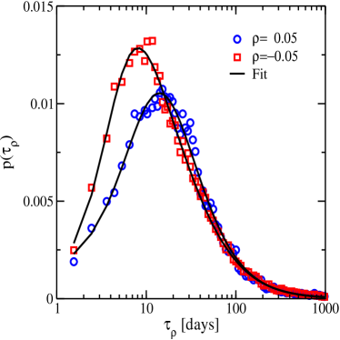
(a) DJIA (1896.5–2001.7)

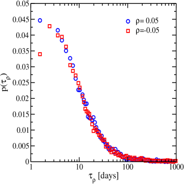
(b) Boeing Airways (1962.1–1999.8)

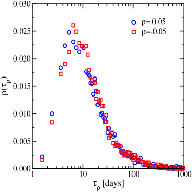
(c) General Electric (1970.0–1999.8)

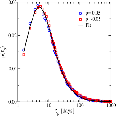
(d) Stock averaged gain and loss distributions

Figure 1: Inverse statistics for detrended closing prices (open symbols) of the DJIA for the time periods indicated. For all cases the return levels used were $\left|\rho\right|=0.05$. The solid lines represent the best fits of Eq. ((1) to the empirical data with the parameters indicated below; (a) DJIA (1896.5–2001.7): $\alpha\approx 0.51$, $\beta\approx 5.23$, $\nu\approx 0.68$ and $t_{0}\approx 0.42$ (loss distribution); $\alpha\approx 0.51$, $\beta\approx 4.53$, $\nu\approx 2.13$ and $t_{0}\approx 10.1$ (gain distribution); (b) Same as (a), but for Boeing Airways; (c) Same as (a), but for General Electric; (d) Stock averaged gain and loss distribution for the companies listed in table 1. The fit is Eq. (1) with values $\alpha\approx 0.60$, $\beta\approx 3.24$, $\nu\approx 0.94$ and $t_{0}\approx 1.09$. Note that the tail exponent $\alpha+1$ is $0.1$ above the “random walk value” of $3/2$.

References

- [1] I. Simonsen, M. H. Jensen and A. Johansen, Eur. Phys. J. 27 (2002) 583.
- [2] M. H. Jensen, A. Johansen and I. Simonsen, Physica A 234 (2003) 338.
- [3] L. Bachelier, Théorie de la Spéculation”, 1900, Annales de l’Ecole normale superiure.
- [4] J.-P. Bouchaud and M. Potters, Theory of Financial Risks: From Statistical Physics to Risk Management (Cambridge University Press, Cambridge, 2000).
- [5] A.Johansen, I.Simonsen and M.H.Jensen, Inverse Statistics for Stocks and Markets, preprint submitted to Quantitative Finance, see also http://xyz.lanl.gov/physics/0511091
- [6] R. J. Schiller, Irrational Exuberance, Princeton University Press, 2000