First Passage Time Densities in Resonate-and-Fire Models

Abstract

Motivated by the dynamics of resonant neurons we discuss the properties of the first passage time (FPT) densities for nonmarkovian differentiable random processes. We start from an exact expression for the FPT density in terms of an infinite series of integrals over joint densities of level crossings, and consider different approximations based on truncation or on approximate summation of this series. Thus, the first few terms of the series give good approximations for the FPT density on short times. For rapidly decaying correlations the decoupling approximations perform well in the whole time domain.

As an example we consider resonate-and-fire neurons representing stochastic underdamped or moderately damped harmonic oscillators driven by white Gaussian or by Ornstein-Uhlenbeck noise. We show, that approximations reproduce all qualitatively different structures of the FPT densities: from monomodal to multimodal densities with decaying peaks. The approximations work for the systems of whatever dimension and are especially effective for the processes with narrow spectral density, exactly when markovian approximations fail.

I Introduction

The first passage time (FPT) is the time $T$ when a stochastic process $x(t)$ leaves an a priory prescribed domain $\Delta$ of its state space for the first time, assumed that $x(t)$ has been started at $t=0$ from a given initial value within $\Delta$. This concept was originally introduced by E. Schrödinger when discussing behavior of Brownian particles in external fields S1915 . A large variety of problems ranging from noise in vacuum tubes, chemical reactions and nucleation HTB1990 to stochastic resonance LBM1991 , behavior of neurons T1988 , and risk management in finance R2001 can be reduced to FPT problems. In majority of applications the attractor of the system’s dynamics lies inside $\Delta$. The escape process is characterized by the noise-induced flux through the absorbing boundary of $\Delta$, i.e. by the probability density $\mathcal{F}(T)$ of the first passage time.

Approaches to find $\mathcal{F}(T)$ are typically based either on the Fokker-Planck equation with an absorbing boundary R1989 or on the renewal theory vK1992 . Despite the long history, explicit expressions for the FPT density are known only for a few cases. These include overdamped particles under the influence of white noise in the force free case, under time-independent constant forces and linear forces T1988 ; TM1977 ; GM1964 ; S1967 , as well as the case of a constant force under colored noise B2004 . Reasonable approximations exist for a few nonlinear forces SH1989 ; LFS+ . The FPT densities of stationary markovian processes have a very habitual form: $\mathcal{F}(T)$ goes through a single maximum and then it decays either exponentially or as a power law. Many neuronal systems do demonstrate such kind of behavior. It was shown already in GM1964 , that the interspike interval (ISI) histograms obtained experimentally from output of some neurons can be reproduced by FPT densities of one dimensional diffusion process.

This kind of description is suitable for overdamped systems, where the relaxation time to the attractor $t_{rel}$ is much smaller than the typical first passage time. At first the local quasiequilibrium is established in the system. The escape occurs then from this equilibrium state and follows with a constant rate $\kappa$ inversely proportional to the mean FPT. This situation is closely related to the Kramer’s problem considering the quasistationary flux over transparent boundary in the low noise limit. The problem is independent of the detailed initial state and of the time the trajectory has spent inside $\Delta$. At times $T$ exceeding $t_{rel}$ the FPT probability density decays exponentially: $\mathcal{F}(T)\sim\exp(-\kappa T)$. Well known examples are chemical systems and nucleation processes, where the rates determine the mean velocity of chemical reactions or of forming overcritical nuclei HTB1990 . Another example are the leaky integrate-and-fire and similar neuronal models, where after the reset the corresponding trajectories approach quickly the stable rest state LGN+2004 .

However, if the time scale separation between the relaxation and escape does not hold, the escape can occur before the establishment of the quasiequilibrium and the rates are time dependent. The first passage time depends sensitively on the initial conditions and the FPT densities have a complex shape different from an exponential decay. In particular this is the case on short time scales $T<t_{rel}$, which attracted growing interest because of recent experiments studying chemical reactions on time scales down to femtoseconds. The flux over the boundary before the establishment of the quasiequilibrium was found to grow in a stepwise manner, for an underdamped potential system staying initially at the bottom of the well SSL+2001 .

Our work is mainly motivated by dynamics of resonant neurons MCD+1970 ; EKH+2004 ; BHR2003 . The voltage variable of such a neuron exhibits damped subthreshold oscillations around the attractive rest state. The characteristic relaxation time to the rest state is large compared to the mean ISI. The escape of the voltage over the excitation threshold is the beginning of a new spike. After spiking the voltage variable is reset to a fixed value far from the rest state and then it can reach the threshold prior relaxation to the rest. The interspike interval densities obtained from the output of resonant neurons show a sequence of decaying peaks separated by intervals whose length is of the order of the period of subthreshold oscillations. In contrast to the Kramer’s rate theory we stress again the nonstationary character of this problem due to the reset to sharp initial conditions.

The multimodal ISI probability densities can be reproduced in models with different mechanisms of subthreshold resonance: in Hodgkin-Huxley model CWW2001 , in excitable FitzHugh-Nagumo model with the stable fix point being a focus SL2002 ; VSS2004 or in the region of a canard bifurcation VUZ+2003 ; MNV2001 . It was also shown that two-component approximations might well mimic the spiking activity of the stochastic Hodgkin-Huxley system T2005 ; TW2005 . All these models have in common that the multimodal FPT density is obtained for stochastic dynamical systems, which have at least two dynamical variables, exhibit weakly, moderately damped or self-amplifying oscillations and after a spike reset to initial values which are not a fixed point. In the noise-free situation these systems were denoted resonate-and-fire neurons I2001 .

In the present work we aim to model excitable behavior with damped subthreshold oscillations. First we present the general exact expression for the FPT density for stochastic processes with differentiable trajectories S1967 ; R1945 ; S1951 ; F1980 . It results in an infinite series of integrals over joint densities of multiple level crossings. The later sum stands for a sequential summing of trajectories excluding all except the ones yielding the first passage. Furthermore, we discuss approximations for FPT densities, which are based either on truncation of this series, or on its approximate summation based on decoupling. We prove the quality of different approximations by explicit calculations for an underdamped harmonic oscillator driven by white or colored Gaussian noise, representing the stochastic resonate-and-fire neurons.

II Exact expression for the first passage time density

Consider a single random variable $x(t)$, whose $t$-dependence is assumed to be differentiable. The first passage problem for $x(t)$ to a boundary $x_{b}$ is a special case of a level crossing problem.

The general theory of level crossings by a random process was originally put forward by S.O. Rice R1945 . He derived an expression for the probability density of recurrence of a stationary random process to a given level in form of the so called Wiener-Rice series S1951 . The exact expression for the first passage time probability density Eq.(7) is analogous to the Wiener-Rice series and was discussed in F1980 , where the main result, our Eq.(7), was proved. We proceed by giving a much more elementary derivation of Eq.(7) which serves as the main instrument in our further investigations.

Let us first discuss the probability $n_{1}(x_{b},t|x_{0},v_{0})dt$ that a continuous differentiable process $x(t)$ crosses the level $x_{b}$ in a time interval between $t$ and $t+dt$ with positive velocity $v(t)=\dot{x}(t)>0$ under initial conditions $x(0)=x_{0},\dot{x}(0)=v_{0}$. Generally the whole set of variables resulting from the markovian embedding of $x(t)$ should be given at $t=0$. For simplicity we consider two dimensional dynamics, generalization for the higher dimensional systems is obvious. Crossing the level with positive velocity will be referred to as an upcrossing in what follows.

If $x(t)$ crosses the barrier within time interval $(t,t+dt)$ with velocity $v>0$, then the value of coordinate at time $t$ should lie in interval $x_{b}-vdt<x(t)<x_{b}$. The probability that $x(t)$ is in this interval equals $\int\limits_{x_{b}-vdt}^{x_{b}}P(x,v,t|x_{0},v_{0},0)dx=|v|P(x_{b},v,t|x_{0},v_{0},0)dt$. Now, the velocity value at the instant of crossing is positive but otherwise arbitrary. Thus we obtain the probability density of an upcrossing by integration over all positive $v$:

$$n_{1}(x_{b},t|x_{0},v_{0},0)=\int\limits_{0}^{\infty}vP(x_{b},v,t|x_{0},v_{0},0)dv.$$ (1)

Eq. (1) can be simply generalized to give the expression for the joint probability density of multiple upcrossings. The probability $n_{p}(x_{b},t_{p};\dots;x_{b},t_{1}|x_{0},v_{0},0)dt_{p}\dots dt_{1}$, that the process $x(t)$ crosses the level $x_{b}$ in each of $p$ time intervals $(t_{1},t_{1}+dt_{1}),\dots,(t_{p},t_{p}+dt_{p})$ is given by:

$$\begin{split}n_{p}(x_{b},t_{p};\dots;x_{b},t_{1}|x_{0},v_{0},0)=\int\limits_{0}^{\infty}dv_{p}\dots\int\limits_{0}^{\infty}dv_{1}&\\ v_{p}\dots v_{1}P(x_{b},v_{p},t_{p};\dots;x_{b},v_{1},t_{1}|x_{0},v_{0},0).&\end{split}$$ (2)

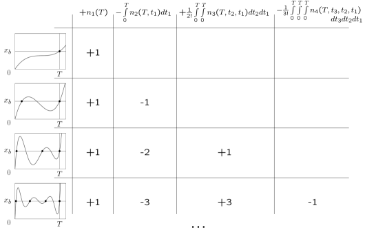
Figure 1: Counting crossings. The $N$th row corresponds to trajectories with exactly $N$ upcrossings. The $p$th column corresponds to the $p$th term of the sum Eq.(6). The number on their intersection gives, how many times a trajectory with exactly $N$ upcrossings is accounted for in the $p$th term. Sum of all numbers in every row is exactly zero.

In what follows we omit $x_{b}$ and initial conditions in expressions for the joint densities of upcrossings. The transition probability densities are connected with joint probability densities according to Bayes’ theorem:

$$\begin{split}&P(x_{p},v_{p},t_{p};\dots;x_{b},v_{1},t_{1}|x_{0},v_{0},0)=\\ &\frac{P_{2p+2}(x_{p},v_{p},t_{p};\dots;x_{b},v_{1},t_{;}x_{0},v_{0},0)}{P_{2}(x_{0},v_{0},0)}.\end{split}$$ (3)

Our aim now is to calculate the first passage time probability density $\mathcal{F}(T)$, that is the fraction of all trajectories starting from the initial point $x_{0}$ with initial velocity $v_{0}$ which perform the upcrossing of the barrier at time $T$ and this upcrossing is the first one. All such trajectories are accounted for in probability density $n_{1}(T)$ (see the first row in Fig. 1). However, $n_{1}(T)$ also accounts for trajectories for which the upcrossing at time $T$ was not the first one, i.e. which had another upcrossing at some earlier time $t_{1}<T$ (row 2 in Fig. 1). Such trajectories should not contribute to $\mathcal{F}(T)$, therefore we should substract them from $n_{1}(T)$. Taking into account that $t_{1}$ can be arbitrary between $0$ and $T$, we get:

$$n_{1}(T)-\int\limits_{0}^{T}n_{2}(T,t_{1})dt_{1}.$$ (4)

This excludes all trajectories which cross $x_{b}$ exactly twice until $T$. However, Eq.(4) does not fully solve the problem since the trajectories crossing $x_{b}$ three times, i.e at time $T$ and at two earlier moments $t_{i}<T,i=1,2$ (row 3 in Fig. 1), are not accounted for correctly. Each such trajectory is counted once in $n_{1}(T)$. The second term in Eq.(4) accounts for the pairs of upcrossings at $T$ and at some $t_{i}<T$. Each trajectory with two additional upcrossings at $t_{i}<T,i=1,2$ is therefore subtracted twice in $\int_{0}^{T}n_{2}(T,t_{1})dt_{1}$. Such trajectories should not contribute to $\mathcal{F}(T)$: in Eq. (4) we subtracted too much and have to add the amount of trajectories with three upcrossings at times $0<t_{i}<T,i=1,2$ and $T$ again:

$$n_{1}(T)-\int\limits_{0}^{T}n_{2}(T,t_{1})dt_{1}+\frac{1}{2!}\int\limits_{0}^{T}\int\limits_{0}^{T}n_{3}(T,t_{2},t_{1})dt_{1}dt_{2}.$$ (5)

The factor $1/2!$ in the last term accounts for the number of permutations of variables $t_{i}$. Generally, if a trajectory crosses the level at time $T$ and at $N$ earlier times $t_{i}<T,i=1,\dots,N$, then in $\frac{1}{p!}\int\dots\int n_{p+1}(T,t_{p},\dots,t_{1})dt_{1}\dots dt_{p}$ it is accounted for exactly $C_{N}^{p}$ times ($C_{N}^{p}$ stands for the number of combinations). Note, that $\sum\limits_{p=0}^{N}(-1)^{p}C_{N}^{p}=(1-1)^{N}=0$. Thus in the alternating sum of the kind Eqs.(4), (5) containing $N+1$ terms, all trajectories crossing $x_{b}$ at time $T$ and having $i=1,2,\dots,N$ additional upcrossings are excluded, however the ones with the larger number of upcrossings are not accounted for correctly. Extending the sum to infinity we exclude all superfluous trajectories, and only trajectories, for which the upcrossing at time $T$ was the first one, remain. Thus the expression for the first passage time probability density reads:

$$\mathcal{F}(T)=\sum\limits_{p=0}^{\infty}\frac{(-1)^{p}}{p!}\int\limits_{0}^{T}\dots\int\limits_{0}^{T}n_{p+1}(T,t_{p},\dots,t_{1})dt_{p}\dots dt_{1}.$$ (6)

Explicitly expressing the joint densities of upcrossings using Eqs.(2),(3), we get

$$\begin{split}\mathcal{F}&(T)=\frac{1}{P_{2}(x_{0},v_{0},0)}\sum\limits_{p=0}^{\infty}\frac{(-1)^{p}}{p!}\int\limits_{0}^{T}\dots\int\limits_{0}^{T}dt_{p}\dots dt_{1}\\ &\int\limits_{0}^{\infty}\dots\int\limits_{0}^{\infty}dvdv_{1}\dots dv_{p}vv_{1}\dots v_{p}\\ &P_{2p+4}(x_{b},v,T;x_{b},v_{p},t_{p};\dots;x_{b},v_{1},t_{1};x_{0},v_{0},0).\end{split}$$ (7)

Eq.(6) connects $\mathcal{F}(T)$, i.e. the solution of the FPT problem with absorbing boundary at $x_{b}$, with all joint densities of upcrossings for the unbounded process. To obtain $n_{p}(t_{p},\dots,t_{1})$ we consider trajectories, which are not absorbed at $x_{b}$, but can return after an upcrossing and then cross $x_{b}$ again and again. The right combination of all these densities of multiple level crossings results in the probability density for the first upcrossing.

An alternative to direct summation of infinite series Eq.(6) is based on an analogue to a cumulant expansion. The times, when the random process $x(t)$ performs upcrossings of $x_{b}$ form a point process, or a system of random points S1967 ; vK1992 . The functions

$$n_{1}(t_{1}),\qquad n_{2}(t_{2},t_{1}),\qquad n_{3}(t_{3},t_{2},t_{1}),\qquad\dots$$ (8)

are the distribution functions of the point process. Since $x(t)$ has finite velocity, the interval between two upcrossings can not be arbitrary small and so $n_{p}(t_{p},\dots,t_{1})$ vanishes if two of its arguments coincide. Such random point process is called a system of nonapproaching points S1967 . In this context $\mathcal{F}(T)$ is interpreted as the waiting-time density of the point process. The last is the probability density for the time $T$ when the first event occur.

The system of random points is completely characterized by its cumulant functions

$$g_{1}(t_{1}),\qquad g_{2}(t_{2},t_{1}),\qquad g_{3}(t_{3},t_{2},t_{1}),\qquad\dots.$$ (9)

Choose an arbitrary natural number $r$, and then fix $r$ arbitrary numbers $z_{1},\dots,z_{r}$ and $r$ positive times $t_{1},\dots,t_{r}$. The cumulant functions are then defined by the relation

$$\begin{split}1+\sum_{p=1}^{\infty}\frac{1}{p!}\sum_{\alpha,\dots,\omega=1}^{r}n_{p}(t_{\alpha},\dots,t_{\omega})z_{\alpha}\dots z_{\omega}=\\ \exp\left(\sum_{p=1}^{\infty}\frac{1}{p!}\sum_{\alpha,\dots,\omega=1}^{r}g_{p}(t_{\alpha},\dots,t_{\omega})z_{\alpha}\dots z_{\omega}\right).\end{split}$$ (10)

We obtain the explicit relations between cumulant and distribution functions of the point process if we differentiate both sides of Eq.(10) over all $z_{i}$ and then set $z_{i}=0,(i=1,\dots,r)$, i.e. if we apply the operator $\partial^{r}/(\partial z_{1}\dots\partial z_{r})\big{|}_{z_{1}=_{\dots}=z_{r}=0}$. Doing so sequentially for $r=1,2,3,\dots$ we get

$$\begin{split}&g_{1}(t_{1})=n_{1}(t_{1}),\\ &g_{2}(t_{2},t_{1})=n_{2}(t_{2},t_{1})-n_{1}(t_{1})n_{1}(t_{2}),\\ &g_{3}(t_{3},t_{2},t_{1})=n_{3}(t_{3},t_{2},t_{1})-3\{n_{1}(t_{1})n_{2}(t_{3},t_{2})\}_{s}\\ &\qquad\qquad\qquad+2n_{1}(t_{1})n_{1}(t_{2})n_{1}(t_{3}),\qquad\dots\end{split}$$ (11)

Here $\{\dots\}_{s}$ denotes the operation of symmetrization of the expression in the brackets with respect to all permutations of its arguments. The coefficients in these forms are the same as in relations between the moments and the cumulants of a random variable.

The relation Eq.(10) does not change its form if we choose different times $t_{1},\dots,t_{r}$, different values $z_{1},\dots,z_{r}$ or change the number $r$. Thus extending $r$ to infinity, allowing $t$ to take all possible values between $0$ and $T$, and choosing $z_{1}=_{\dots}=z_{r}=-1$ we get from Eq.(10)

$$1+{\displaystyle\sum\limits_{p=1}^{\infty}\frac{(-1)^{p}}{p!}\int\limits_{0}^{T}\dots\int\limits_{0}^{T}n_{p}(t_{p},\dots,t_{1})dt_{p}\dots dt_{1}=}$$

$$\exp\left({\displaystyle\sum\limits_{p=1}^{\infty}\frac{(-1)^{p}}{p!}\int\limits_{0}^{T}\dots\int\limits_{0}^{T}g_{p}(t_{p},\dots,t_{1})dt_{p}\dots dt_{1}}\right).$$

It is easy to verify, that the derivative $(-d/dT)$ of the expression on the left hand side of Eq.(II) is exactly the expression on the right hand side of Eq.(6). Thus differentiating the right hand side of Eq.(II) over $T$ we obtain the expression for the waiting-time density $\mathcal{F}(T)$ through the cumulant functions of the point process:

$$\mathcal{F}(T)=S^{\prime}(T)e^{-S(T)}$$ (13)

with

$$S(T)=-\sum_{p=1}^{\infty}\frac{(-1)^{p}}{p!}\int\limits_{0}^{T}\dots\int\limits_{0}^{T}g_{p}(t_{p},\dots,t_{1})dt_{p}\dots dt_{1}.$$ (14)

Eqs.(9)-(II) are general expressions which hold for systems of random points, defined by distribution functions Eq.(8) of any kind. So are also Eqs.(6) and (13), (14), which give the waiting-time density for arbitrary point process. In particular, for the random points being the times, when a differentiable random process crosses the level $x_{b}$, the distribution functions $n_{p}(t_{p},\dots,t_{1})$ are given by the joint densities of upcrossings Eq.(2). Then Eqs.(6) and (13), (14) together with Eq.(2) express the first passage time density for this differentiable random process. The function $S^{\prime}(T)$ can be interpreted as a the time-dependent escape rate.

These are the exact results for the FPT probability density of any continuous differentiable random process. Though these results were employed for mathematical proofs, up to our knowledge these infinite series of multiple integrals was never used for explicit calculations. We proceed to show, that Eqs.(6) and (13), (14) can be a starting point for several approximations. As often in the case of infinite series, the useful approximations can be based either on the truncation of the series after several first terms calculated exactly, or by approximation of the higher order terms through the lower order ones what might lead to a closed analytical form. Truncation approximations for Eq.(6) are not normalized, hold only on short time scales, and diverge at longer times (due to the miscount of trajectories with several upcrossings). The approximations of the second type are based on a subsummation in Eq.(14) for $S(T)$. They are normalized and can be used in the whole time domain. Note, only approximations guaranteeing positive rates $S^{\prime}(T)$ are reasonable. Thus the set of possible approximations for the series Eq.(14) is rather restricted.

III Noisy driven harmonic oscillator: resonate-and-fire

The model we have in mind is the resonate-and-fire model of a neuron I2001 . This is the least complicated model accounting for the resonant properties of neurons in terms of an equivalent RLC circuit MCD+1970 ; EKH+2004 . In this way it is directly related to the leaky integrate-and-fire model also based on the electrical analogy. Alternatively the model can be interpreted as a systematic and linearized reduction of Hodgkin-Huxley type dynamics K1999 . For the sake of simplicity we neglect the absolute refractory time. Under this assumption the model is equivalent to the underdamped harmonic oscillator with the threshold and reset, what makes the results applicable in many other domains of science. We change by time scale and variable transformations to dimensionless parameters and variables. The dynamics of the voltage variable $x(t)$ is given by:

$$\dot{x}=v;\qquad\dot{v}=-\gamma v-\omega_{0}^{2}x+\eta(t).$$ (15)

We fix the frequency $\omega_{0}=1$, choose initial conditions for $x$ and its velocity $v$ to be $x_{0}=-1,v_{0}=0$ and set the threshold at $x_{b}=1$. In the present paper we consider two types of noisy drive: (i) the white noise $\eta(t)=\sqrt{2D}\xi(t)$, and (ii) the Ornstein-Uhlenbeck noise $\dot{\eta}=-\tau^{-1}\eta+\sqrt{2D}\tau^{-1}\xi(t)$, with $\xi(t)$ being the white Gaussian noise of intensity 1. First we concentrate on the case (i) of white noise driving.

Because of the linearity of the system Eq.(15) all joint probability densities are Gaussian and have the form R1989 :

$$P_{n}(\vec{Q})=\frac{1}{(2\pi)^{n/2}\sqrt{\det\hat{C}_{n}}}\exp\left(-\frac{\vec{Q}\hat{C}_{n}^{-1}\vec{Q}}{2}\right).$$ (16)

Here $\vec{Q}=(q_{1}(t_{1}),\dots,q_{n}(t_{n}))$ is an $n$-dimensional vector, whose $i$th component is the value of coordinate $x(t_{i})$ or of velocity $v(t_{i})$ at the moment $t_{i}$. $\hat{C}_{n}$ is symmetric $n\times n$ correlation matrix. Its elements are correlation functions between corresponding components of vector $\vec{Q}$ : $c_{ij}=c_{ji}=\langle q_{i}(t_{i})q_{j}(t_{j})\rangle$.

Correlation functions for the system Eq.(15) are easily obtained using Fourier transform and Wiener-Khinchin theorem R1989 . For the case of white noise driving and in an underdamped regime ($\gamma<2\omega_{0}$) $r_{xx}(t)=\langle x(t^{\prime})x(t^{\prime}+t)\rangle=\frac{D}{\gamma\omega_{0}^{2}}e^{-\frac{\gamma}{2}t}\left(\frac{\gamma}{2\Omega}\sin(\Omega t)+\cos(\Omega t)\right)$, with $\Omega=\sqrt{|\omega_{0}^{2}-\frac{\gamma^{2}}{4}|}$. In overdamped case ($\gamma>2\omega_{0}$) the expression for $r_{xx}(t)$ is the same, except the trigonometric functions are replaced with hyperbolic ones. Further, $r_{xv}(t)=r^{\prime}_{xx}(t)$ and $r_{vv}(t)=-r^{\prime\prime}_{xx}(t)$.

Then $n_{1}(T)$ is obtained from Eq.(1) in closed analytical form:

$$\begin{split}n_{1}&(T)=\frac{\sigma_{x}\sigma_{v}}{2\pi\mu_{22}\sqrt{\det\hat{C}_{4}}}\exp\left[\frac{\sigma_{x}^{2}v_{0}^{2}+\sigma_{v}^{2}x_{0}^{2}}{2\sigma_{x}\sigma_{v}}\right]\\ &\exp\left[-\frac{1}{2}\sum\limits_{i,j\neq 2}\mu_{ij}q_{i}q_{j}\right]\left[1-\sqrt{\pi}\alpha e^{\alpha^{2}}\mathrm{erfc}(\alpha)\right].\end{split}$$ (17)

Here $\mu_{ij}=\mu_{ji}$ are elements of the inverse correlation matrix $(\hat{C}_{4})^{-1}$, $q_{i}$ are components of the vector $\vec{Q}=(x(T),v(T),x_{0}(0),v_{0}(0))$. The dispersions of $x$ and $v$ are $\sigma_{x}^{2}=r_{xx}(0)=D/\gamma\omega_{0}^{2}$, $\sigma_{v}^{2}=r_{vv}(0)=D/\gamma$. We have introduced $\alpha=\left(\sum\limits_{i\not{=}2}\mu_{2i}q_{i}\right)/\sqrt{2\mu_{22}}$. Finally, $\mathrm{erfc}(x)$ is a complementary error function.

For the joint densities of multiple upcrossings $n_{p}(t_{p},\dots,t_{1})$ no closed expressions can be obtained. We evaluate the integral over $v_{1}$ in Eq.(2) analytically and then perform numerical integration of the resulting expression over $v_{2},\dots,v_{p}$ to obtain $n_{p}(t_{p},\dots,t_{1})$. The integrals over time in the expressions for $\mathcal{F}(T)$ are also evaluated numerically.

IV Truncation approximations

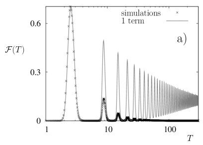
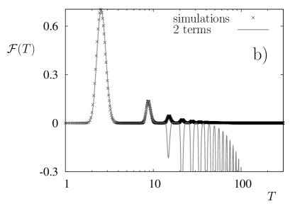
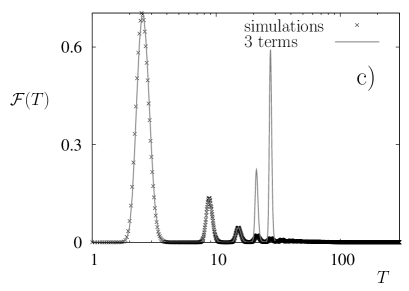
Figure 2: FPT density for harmonic oscillator driven by white Gaussian noise, $\omega_{0}=1,\gamma=0.01,D=0.02,x_{0}=-1,v_{0}=0,x_{b}=1$. Simulation results shown with black crosses and truncation approximations with gray line: (a) 1 term Eq.(1), (b) 2 terms Eq.(4) and (c) 3 terms Eq.(5). The mean FPT obtained from simulations equals $14.6$, the median of distribution lies by $3.2$. Note the logarithmic scale.

The first passage time density $\mathcal{F}(T)$ for the harmonic oscillator driven by white Gaussian noise obtained from simulations is depicted with black crosses in Fig.2. Parameters are chosen to be $\gamma=0.01,D=0.02$. In this case of very small friction the correlation functions of the process oscillate with period $T_{p}=2\pi/{\sqrt{\omega_{0}^{2}-\gamma^{2}/4}}$ and decay slowly within the relaxation time $t_{rel}=2/\gamma$. A typical trajectory is smooth and shows almost regular oscillations with fluctuating phase and amplitude. The probability to reach $x_{b}$ is higher in the maxima of the subthreshold oscillations. The initial phase of these oscillations is fixed by sharp initial conditions. Thus on shorter time scales $\mathcal{F}(T)$ shows the multiple peaks following with the frequency of damped oscillations $\Omega=\sqrt{\omega_{0}^{2}-\gamma^{2}/4}$. On long times $T\gg t_{rel}$ the quasiequilibrium establishes and FPT density decays exponentially. The number of visible peaks depends on the relation between $t_{rel}$ and the period of oscillations $T_{p}$ and is given by the number of periods elapsing before the quasiequilibrium is achieved. For parameter values as in Fig.2 $t_{rel}=200$, what corresponds to about 30 periods $T_{p}=6.28$.

Let us consider truncation approximations for the series Eq.(6). The first approximation is given by the first term $n_{1}(T)$, the second approximation by 2 terms, Eq.(4), and the third by 3 terms, Eq.(5). The higher order approximations entail the numerical estimation of highdimensional integrals, which at some stage leads to a computational effort larger than the one necessary for a direct simulation. Therefore we restrict ourselves to the 1-, 2- and 3- terms approximations.

The result of the 1 term approximation is shown in Fig.2(a) with a gray line. The first peak of the FPT density is reproduced almost exactly. All further peaks are overestimated, because all trajectories performing multiple upcrossings of $x_{b}$ are included. On long times the process becomes stationary and the first approximation tends to a constant value $\lim_{T\rightarrow\infty}n_{1}(T)=n_{0}$. This is the mean frequency of upcrossings for a stationary process, also known as the Rice frequency R1945 . The general expression for $n_{0}$ reads

$$n_{0}=\frac{1}{2\pi}\left(-\frac{r^{\prime\prime}_{xx}(0)}{r_{xx}(0)}\right)^{1/2}e^{-x_{b}^{2}/2r_{xx}(0)}.$$ (18)

In our case of a harmonic oscillator driven by white noise $n_{0}=(\omega_{0}/2\pi)\exp{(-\gamma x_{b}^{2}\omega_{0}^{2}/2D)}$. In the stationary regime the mean interval between two consecutive upcrossing $T_{R}$ is given by the inverse of the Rice frequency $T_{R}=1/n_{0}$. For the chosen parameter values $T_{R}=8.06$.

The second approximation (gray line in Fig.2(b)) reproduces almost exactly the first two peaks of FPT density. Then it becomes negative, because in Eq.(4) trajectories performing 2 and more superfluous upcrossings are subtracted too many times. Moreover the second approximation tends to minus infinity for $T\rightarrow\infty$. The third approximation reproduces well the three first peaks of $\mathcal{F}(T)$, and then diverges tending to plus infinity.

Note that the mean first passage time obtained numerically equals $14.6$ for these parameter values, and the median of the distribution lies by $3.2$. Thus the first three approximations reproduce the most part of the FPT probability density.

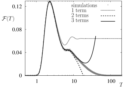
Figure 3: FPT density for harmonic oscillator driven by white Gaussian noise, $\omega_{0}=1,\gamma=0.8,D=0.44,x_{0}=-1,v_{0}=0,x_{b}=1$. Simulation results shown with gray crosses; 1 term approximation Eq.(1) with a dot line, 2 terms approximation Eq.(4) with a dashed line, and 3 terms approximation Eq.(5) with a solid line. The mean FPT obtained from simulations equals $13.1$, the median of distribution lies by $9.1$. Note the logarithmic scale.

The behavior of $\mathcal{F}(T)$ for the harmonic oscillator with higher damping $\gamma=0.8$, stronger noise intensity $D=0.44$, and other parameters as in Fig.2 is presented in Fig.3. For these parameter values the relaxation time $t_{rel}=2.5$ is less than the period $T_{p}=6.86$. Therefore the FPT density is practically monomodal with a single maximum and a small shoulder separating it from the exponential tail. The numerically obtained $\mathcal{F}(T)$ is shown with gray crosses, the 1 term truncation with a dot line, the 2 terms truncation with a dashed line, and the 3 terms truncation with a solid line. The truncation approximations reproduce again the most part of the distribution: the mean FPT equals 13.1 and the median lies by 9.1.

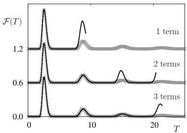
Figure 4: The same as in Fig.2, however the truncations are correctly normalized by Eq.(19). Simulation results shown with gray crosses; the truncations with solid lines. The curves for normalized 1,2, and 3 terms truncations are vertically shifted by 0.6 for the sake of clarity.

Thus the truncation approximations reproduce the FPT density on short times but are not normalized and diverge on large times. However, one can force the normalization in truncations as follows

$$\left|\mathcal{F}_{trunc}(T)\right|\Theta\left(1-\int_{0}^{T}\left|\mathcal{F}_{trunc}(t)\right|dt\right).$$ (19)

Here $\mathcal{F}_{trunc}(T)$ is a truncated series for the FPT density, it is given by Eqs.(1),(4), and (5) for 1,2, and 3 terms truncations respectively. $\Theta(t)$ is the Heaviside step function: the expression Eq.(19) turns to zero as soon as the integral over the absolute value of $\mathcal{F}_{trunc}(T)$ exceeds 1.

In Fig.4 we show the FPT density for the same parameter values as in Fig.2. Simulation results are shown with crosses, and approximations obtained from Eq.(19) with 1,2, and 3 terms by solid lines. The probability distributed over the long exponential tail in the real FPT density, is concentrated in the positive artefact posed on intermediate times in the normalized truncations. Hence the mean FPT computed from such approximations is always strongly underestimated.

The more terms are included, the more precise truncations become. However one has to confine oneself to a few terms, since the calculation of higher order terms implies the computation of multiple integrals and is not more effective than simulations. Therefore the truncation approximations are good, when the most part of the FPT probability is concentrated in the first few peaks, i.e. when the barrier value is low or the noise is strong.

V Decoupling approximations

Decoupling approximations for Eq.(6) or Eq.(14) are based on approximate expressions of the higher order terms through the lower order ones, what may lead to a closed analytical form. Thereby infinitely many approximate terms are included.

The simplest way to obtain such an approximation is to neglect all correlations between upcrossings. This means to neglect all terms in Eq.(14) except for the first one, and leads to

$$S(T)=\int\limits_{0}^{T}n_{1}(t)dt.$$ (20)

Equivalently, neglecting all correlations corresponds to the factorization of $n_{p+1}(T,t_{p},\dots,t_{1})$ into a product of one-point densities $n_{1}(T)n_{1}(t_{p})\dots n_{1}(t_{1})$ in Eq.(6). Then the series, Eq.(6) sums up into $\mathcal{F}(T)\approx n_{1}(T)\exp\left(-\int_{0}^{T}n_{1}(t)dt\right)$, which is equivalent to Eqs.(13),(20). This approximation will be refereed to as the Hertz approximation since the form of ${\cal F}(T)$ resembles the Hertz distribution H1909 . It is an approximation of first order, since it takes the first term of the series exactly, and all other terms are approximated through this first one.

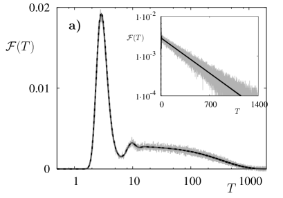
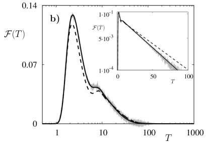
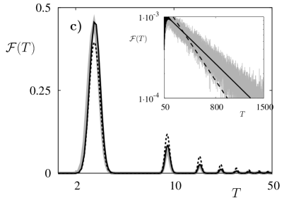
Figure 5: FPT probability density for harmonic oscillator driven by Gaussian white noise. Simulation results are shown with a gray line, Hertz approximation with a black dashed line, and Stratonovich approximation with a black solid line. Note the logarithmic scale in $T$. The insets show the same curves on the logarithmic scale in ${\cal F}(T)$. The parameters are: $\omega_{0}=1,x_{0}=-1,v_{0}=0,x_{b}=1$, a) $\gamma=0.8,D=0.1,t_{rel}=2.5,T_{R}=343$, b) $\gamma=0.8,D=0.44,t_{rel}=2.5,T_{R}=15.6$, c) $\gamma=0.08,D=0.01,t_{rel}=25,T_{R}=343$

The second order approximation should therefore account the first and the second terms exactly and approximate all higher terms through these two. The general form of $\mathcal{F}(T)$ in terms of the cumulant functions Eq.(13) ensures the right normalization, irrespective of the way how $S(T)$ is approximated. However the simple truncation of the series Eq.(14) after the second term does not ensure the positive escape rate $S^{\prime}(T)$.

The second order approximation guaranteeing $S^{\prime}(T)>0$ was proposed by Stratonovich in the context of peak duration S1967 . The first and the second cumulant functions are taken exactly, and the higher ones are approximated by the combinations of these two:

$$\begin{split}g_{p}(t_{p},\dots,t_{1})\approx&(-1)^{p-1}(p-1)!n_{1}(t_{p})\dots n_{1}(t_{1})\\ &\{R(t_{1},t_{2})R(t_{1},t_{3})\dots R(t_{1},t_{p})\}_{s}.\end{split}$$ (21)

Here $\{\dots\}_{s}$ is again the operation of symmetrization. $R(t_{i},t_{j})$ is the correlation coefficient of upcrossings

$$R(t_{i},t_{j})=1-\frac{n_{2}(t_{i},t_{j})}{n_{1}(t_{i})n_{1}(t_{j})}.$$ (22)

Note, that $R(t_{1},t_{1})=1$ and $R(t_{i},t_{j})\rightarrow 0$ for large values of $|t_{i}-t_{j}|$.

The approximation of the cumulant functions in form Eq.(21) can be motivated by the following argument. Consider Eq.(10) with $r=1$. Recall that the joint densities of upcrossings vanish for coinciding arguments: $n_{p}(t_{1},\dots,t_{1})=0$. Thus it follows from Eq.(10):

$$\ln(1+n_{1}(t_{1})z_{1})=\sum\limits_{p=1}^{\infty}\frac{1}{p!}g_{p}(t_{1},\dots,t_{1})z_{1}^{p}.$$

The above expression should hold for arbitrary $z_{1}$. Therefore expanding the logarithm in series, and equating the coefficients by the same powers of $z_{1}$ on the both sides, one obtains the identity

$$g_{p}(t_{1},\dots,t_{1})=(-1)^{p-1}(p-1)!n_{1}^{p}(t_{1}).$$ (23)

Eq.(23) is exact for all arguments coinciding. Eq.(21) gives a correction to it, when the arguments differ.

Substitution of Eq.(21) into Eq.(14) delivers then the Stratonovich approximation for $\mathcal{F}(T)$ in form Eq.(13), now with the time-dependent escape rate being

$$S(T)=-\int\limits_{0}^{T}n_{1}(t)\frac{\ln\left[1-\int_{0}^{T}R(t,t^{\prime})n_{1}(t^{\prime})dt^{\prime}\right]}{\int_{0}^{T}R(t,t^{\prime})n_{1}(t^{\prime})dt^{\prime}}dt.$$ (24)

Let us now discuss the domains of applicability for these approximations. The Hertz approximation Eq.(20) holds if all correlations decay considerably within the typical time interval between upcrossings $T_{R}$. The decay of correlations is described by the relaxation time $t_{rel}=2/\gamma$ of the process. Therefore, the Hertz approximation holds for $t_{rel}\ll T_{R}$.

The Stratonovich approximation is applicable when the argument of the logarithm in Eq.(24) is positive, $1-\int_{0}^{T}[n_{1}(t^{\prime})+n_{1}(t)^{-1}n_{2}(t^{\prime},t)]dt^{\prime}>0$. Using the fact that $n_{2}(t^{\prime},t)/n_{1}(t)$ tends to $n_{1}(t^{\prime})$ for $|t-t^{\prime}|>t_{rel}$ and tends to zero for $|t-t^{\prime}|\rightarrow 0$ we get as a rough estimate for the validity region of Eq.(24) $t_{rel}<T_{R}$.

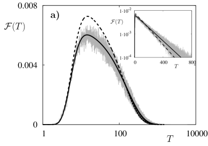
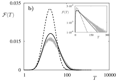
Figure 6: Same as in Fig. 5 however for the case of stronger friction. The parameters are a) $\gamma=3.0,D=0.5,\omega_{0}/\gamma=0.33$, b) $\gamma=10.0,D=5.5,\omega_{0}/\gamma=0.1$ and other parameters as in Fig. 5.

Let us now turn to the results for the harmonic oscillator Eq.(15) with white noise driving. In Figs.5 and 6 the FPT probability density obtained from simulations is depicted with a gray line, the Hertz approximation Eq.(20) with a black dashed line, and the Stratonovich approximation Eq.(24) with a black solid line.

In Fig.5(a) the parameters are chosen to be $\gamma=0.8,D=0.1$, corresponding to moderate friction and moderate noise intensity. For given parameter values $t_{rel}=2.5$ and $T_{R}=343$, so that $t_{rel}\ll T_{R}$, both Hertz and Stratonovich approximations hold and reproduce well the FPT density in the whole time domain.

In the case of moderate friction and stronger noise the upcrossings become more frequent and $T_{R}$ decreases. The FPT changes its form to practically monomodal. An example is given in Fig.5(b) with $\gamma=0.8,D=0.44$ which correspond to $t_{rel}=2.5$ and $T_{R}=15.6$. The Stratonovich approximation complies very well with simulations, while the Hertz approximation fails to reproduce the details of the distribution: It underestimates $\mathcal{F}(T)$ on short times, and shows slower exponential decay in the tail than the one observed in simulations (see the inset).

Finally, for small friction and week noise the upcrossings are rare, but the relaxation time is large. The FPT probability density exhibits multiple decaying peaks. In Fig.5(c) $\gamma=0.08,D=0.01$ corresponding to $t_{rel}=25,T_{R}=343$. Again, the Stratonovich approximation performs well, while the Hertz approximation underestimates the first peak, overestimates all further peaks and decays in the tail faster than the simulated FPT density.

For the large $T$, $\mathcal{F}(T)$ decays exponentially, $\mathcal{F}(T)\propto\exp(-\kappa T)$. The decrement of this decay is obtained from long time asymptotic: $\kappa T=\lim_{T\rightarrow\infty}S(T)$. Thus, in the Hertz approximation Eq.(20) one gets $\kappa_{H}=\lim_{T\rightarrow\infty}(1/T)\int_{0}^{T}n_{1}(t)dt=n_{0}T/T=n_{0}$. The behavior in the Stratonovich approximation Eq.(24) is determined by $\lim_{t,t^{\prime}\rightarrow\infty}\int_{0}^{T}R(t,t^{\prime})n_{1}(t^{\prime})dt^{\prime}\approx n_{0}\tau_{cor}$ with $\tau_{cor}$ given by $\tau_{cor}=\lim\limits_{t\rightarrow\infty}\int_{0}^{\infty}R(t,t^{\prime})dt^{\prime}$. Note that $\tau_{cor}$ is not necessary positive because of oscillating correlation coefficient. Inserting this expression into Eq.(24) and expanding the logarithm up to the second term we get $\kappa_{S}=n_{0}(1+\frac{1}{2}n_{0}\tau_{cor})$ providing the second order correction to $\kappa_{H}$. The value of $\tau_{cor}$ for the parameter set as in Fig.5(a) is $\tau_{cor}=-2.4$, for parameters as in Fig.5(b) $\tau_{cor}=5.09$, and for parameters as in Fig. 5(c) $\tau_{cor}=-431.99$. The long time asymptotic obtained with these $\tau_{cor}$ values reproduce fairly well the decay patterns found numerically.

In the overdamped regime ($\gamma>2\omega_{0}$) the condition $t_{rel}<T_{R}$ is always fulfilled. Nevertheless the validity region of our approximations is limited. With increasing friction the process $x(t)$ approaches to the markovian one (it is markovian in the overdamped limit $\omega_{0}/\gamma\ll 1$). For such processes the pattern of upcrossings is not homogeneous, but shows rather well separated clusters of upcrossings S1967 . Essentially in the markovian limit the property, that upcrossings form a system of nonapproaching random points is violated. The upcrossings within a single cluster are not independent even if their mean density $n_{0}$ is low, so that the quality of approximations decreases. This fact is illustrated in Fig.6. In the overdamped regime the correlation functions decay monotonously, and the FPT densities are always monomodal. The parameters in Fig.6(a) are $\gamma=3.0,D=5.5$, so that $\omega_{0}/\gamma=0.33$. Eqs.(13),(24) continue to give a good approximation for $\mathcal{F}(T)$, while the Hertz approximation becomes inaccurate. Further increase in friction, for example $\gamma=10.0,D=5.5$ as in Fig.6(b) corresponding to $\omega_{0}/\gamma=0.1$, makes the process to approach the Markovian limit. The Stratonovich approximation starts to be inaccurate, and the Hertz approximation fails.

VI Truncation versus decoupling approximations.

In the two previous sections we have seen, that truncation approximations reproduce the FPT density on short time scales. In contrast, the decoupling approximations reproduce FPT densities in the whole time domain and posses the right normalization. At the first glance, it may seem that the decoupling approximations excel the direct truncations and should be preferably used in applications. However, it depends on the problem one has to solve, and sometimes the truncations turn out to be useful.

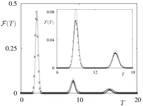
Figure 7: FPT density for harmonic oscillator driven by white Gaussian noise, $\omega_{0}=1,\gamma=0.08,D=0.01,x_{0}=-1,v_{0}=0,x_{b}=1$. Simulation results are shown with crosses, the 3 terms approximation with black line, and the Stratonovich approximation with gray line. The inset shows the magnification of a part of the curve.

One such situation was already mentioned. If the noise intensity is high or the barrier value is low, then the upcrossings occur frequently, and the decoupling approximations can not be applied. For example, for parameter values as in Fig.2, the relaxation time is $t_{rel}=200$, and the mean interval between upcrossings $T_{R}=8.07$. Thus $t_{rel}>T_{R}$, and both Hertz and Stratonovich approximations fail. Nevertheless, the most part of the FPT density is concentrated in the first few peaks in this case, and is well reproduced by the truncation approximations, as shown in Figs.2 and 4.

One can also be interested in a very accurate approximation for the FPT density on short times. The truncations deliver better results on short times than the decoupling approximations. For example, in Fig.7 the simulation results are compared with the 3 terms truncation and the Stratonovich approximation for the same parameter values as in Fig.5(c). Both approximation reproduce very accurate the first peak in the FPT density. However, the 3 terms truncation is much more accurate in estimation of the second and third peaks (see the inset in Fig.7).

This can be easily understood. The Stratonovich approximation takes $n_{1}(t_{1})$ and $n_{2}(t_{2},t_{1})$ exactly, and approximates all higher order densities through these two. On times, when the first peak occurs, $n_{2}(t_{2},t_{1})$ is negligibly small. Then from Eqs.(21),(22) we obtain $g_{p}(t_{p},\dots,t_{1})\approx(-1)^{p-1}(p-1)!n_{1}(t_{p})\dots n_{1}(t_{1})$. Substitution of this expression into Eq.(10) gives then $n_{p}(t_{p},\dots,t_{1})\approx 0$ for $p>1$. Thus on these times the Stratonovich approximation just coincides with the 1 term truncation, and so reproduces the first peak very accurately. On times, when the second peak in the FPT density occurs, $n_{2}(t_{2},t_{1})$ is significantly different from zero. Hence all approximated $n_{p}(t_{p},\dots,t_{1}),p>2$ turn out to be nonvanishing as well, while the real values for these functions are negligibly small on these times. Thus the accuracy of the Stratonovich approximation decreases in the second peak. From analogous reasoning it becomes clear, that the Hertz approximation is already inaccurate in estimation of the first peak.

VII Harmonic oscillator driven by colored noise

Expressions Eq.(6) and Eqs.(13),(24) can be used to obtain the FPT density for a random process $x(t)$, if the joint probability densities of $x$ and its velocity $v$ Eq.(2) exist. Thus it is necessary that the process $x(t)$ is continuous and differentiable at any time, but there are no further restrictions on dimension and form of the system. The truncation and decoupling approximations deliver good results for the FPT density in their validity regions independently of the character of the noisy drive. In particular the case of correlated input signals (colored noise driving) is of importance in neuroscience. For example, synaptic filtering of the input spike train may lead to an exponentially correlated input signal.

Therefore we consider as another example a resonate-and-fire neuron Eq.(15) driven by the Ornstein-Uhlenbeck noise. The correlation time of the process is $\tau$, the variance $D/\tau$, and the correlation function $\langle\eta(t)\eta(t+t^{\prime})\rangle=(D/\tau)\exp(-t^{\prime}/\tau)$. In the limit $\tau\rightarrow 0$ the process tends to the white noise of intensity $2D$. The correlation functions $r_{xx}(t),r_{xy}(t),r_{yx}(t),r_{xv}(t)=r^{\prime}_{xx}(t),r_{vv}(t)=-r_{xx}^{\prime\prime}(t),r_{yv}(t)=r_{yx}^{\prime}(t),r_{vy}(t)=-r_{xy}^{\prime}(t)$ can be obtained using Fourier transform as it was done for the white noise case in Section III.

Then $n_{1}(T)$ is again obtained analytically and has the form given by Eq.(17). Now $\mu_{ij}=\mu_{ji}$ are elements of the inverse correlation matrix $(\hat{C}_{5})^{-1}$, $q_{i}$ are components of vector $\vec{Q}=(x(T),v(T),x_{0}(0),v_{0}(0),\eta_{0}(0))$. The factor $\alpha$ is defined in the same way as it was done in Section III.

For simplicity, we assumed sharp initial conditions for the noise variable, i.e. $\eta$ is reset after every spike to a fixed value $\eta_{0}$. The alternative assumption, that the neuron variables $x,v$ are reset to their initial values once $x(t)$ reaches the thereshold without resetting $\eta(t)$, might be more realistic B2004 . In this case all probability densities should be averaged with respect to the stationary density of noise values upon firing. However, as an example, we confine ourselves to consideration of sharp initial conditions for the noise: $P(\eta,t=0)=\delta(\eta-\eta_{0})$.

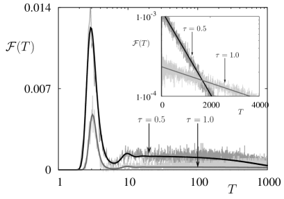
Figure 8: Simulation results and the Hertz approximation for the FPT probability density for harmonic oscillator driven by Ornstein-Uhlenbeck noise with correlation times $\tau=0.5$ (upper curves) and $\tau=1.0$ (lower curves) and other parameters as in Fig.5(a). Note the logarithmic scale in $T$. The inset shows the same curves on the logarithmic scale in ${\cal F}(T)$.

In Fig.8 we show simulated FPT probability density and the Hertz approximation for the harmonic oscillator driven by the Ornstein-Uhlenbeck noise. We choose two different values of the correlation time: $\tau=0.5$ and $\tau=1.0$. The reset value for the noise is $\eta_{0}=0$, and other parameters are as in Fig.5(a). The noise intensity decreases with increasing $\tau$, hence the mean FPT growth. Though $\mathcal{F}(T)$ preserves its structure as a whole, for larger values of $\tau$ the height of the main peak decreases and the weight of the exponential tail growth. For given values of the correlation time $T_{R}=829.2$ and $T_{R}=4247.1$ respectively, what significantly exceeds $t_{rel}$. Thus in both cases the Hertz approximation is absolutely sufficient.

VIII Summary

Motivated by studies of resonant neurons, we consider the first passage time problem for systems with subthreshold oscillations and nonnegligible relaxation times after a reset. The joint densities of multiple upcrossings for such a process $x(t)$ can be obtained in the case of differentiable trajectories. The FPT density for $x(t)$ is expressed in terms of an infinite series of multiple integrals over all joint densities of upcrossings, or equivalently, in terms of the cumulant functions.

We consider two types of approximations for this infinite series. The truncation approximations include the first few terms of the series calculated exactly. They reproduce well the FPT density on short and intermidiate times and can be used, when the most part of the FPT probability is concentrated in the first few peaks, i.e. when the barrier value is low or the noise is strong.

The decoupling approximations can be derived for the case of weakly correlated upcrossings. The higher order cumulant functions are expressed through the lower order ones, and then infinitely many terms sum up to the closed expression for $\mathcal{F}(T)$. The Hertz approximation (the one neglecting all correlations between upcrossings) is absolutely sufficient for the case of moderate friction and moderate noise intensity. The Stratonovich approximation (approximating the higher order cumulant functions through the first and the second ones) performs even better and does not loose the accuracy for high noise intensities or in the slightly overdamped regime.

We illustrate our results by the noise driven harmonic oscillator, with the threshold value at $x_{b}$ and reset to sharp initial conditions, i.e. the resonate-and-fire model of a neuron. The validity regions of the approximations cover all different types of subthreshold dynamics. Thus the approximations reproduce all qualitatively different structures of the FPT densities: from monomodal through bimodal to multimodal densities with several decaying peaks. The approximations hold for systems of whatever dimension. We illustrate this by the harmonic oscillator driven by the Ornstein-Uhlenbeck noise.

Though we applied the theory to the harmonic oscillator (resonate-and-fire model), the linearity of the system is in general not required. The joint distributions of $x(t)$ and its velocity should exist, i.e. $x(t)$ should be differentiable in time. No further restrictions on the form and dimension of the system are implied.

References

- (1) E. Schrödinger, Physik. Z. 16, 289 (1915).
- (2) P. Hänggi, P. Talkner, and M. Borkovec, Rev. Mod. Phys. 62, 251 (1990).
- (3) A. Longtin, A. Bulsara, and F. Moss, Phys. Rev. Lett. 67, 656 (1991).
- (4) H.C. Tuckwell, Introduction to Theoretical Neurobiology, vol. 2 (Cambridge University Press, Cambridge UK, 1988).
- (5) S. Redner, A Guide to First-Passage Processes (Cambridge University Press, Cambridge UK, 2001).
- (6) H. Risken, The Fokker-Planck Equation (Springer, Berlin, 1996).
- (7) N. G. van Kampen, Stochastic Processes in Physics and Chemistry (North-Holland, Amsterdam 1992).
- (8) V.I. Tikhonov, M.A. Mironov, Markovian Processes (Sov. Radio, Moscow, 1977).
- (9) G.L. Gerstein, and B. Mandelbrot, Biophys. J. 4, 41 (1964).
- (10) R.L. Stratonovich, Topics in the Theory of Random Noise, vol. 2 (Gordon and Breach, New York, 1967).
- (11) B. Lindner, Phys. Rev. E 69, 022901 (2004).
- (12) D. Sigeti and W. Horsthemke, J. Stat. Phys. 54, 1217 (1989).
- (13) S. Liepold, J.A. Freund, L. Schimansky-Geier, A. Neiman, and D. Russell, Journ. Theor. Biophys., in print.
- (14) B. Lindner, J. García-Ojalvo, A. Neiman, and L. Schimansky-Geier, Phys. Reports 392, 321 (2004).
- (15) S.M. Soskin, V.I. Sheka, T.L. Linnik, and R. Mannella, Phys. Rev. Lett., 86, 1665 (2001).
- (16) A. Mauro, F. Conti, F. Dodge, and R. Schor, J. General Physiol. 55, 497 (1970).
- (17) I. Erchova, G. Kreck, U. Heinemann, and A.V.M. Herz, J. Physiol. 560, 89 (2004).
- (18) N. Brunel, V. Hakim and M.J.E. Richardson, Phys. Rev. E, 67, 051916 (2003).
- (19) D.T.W. Chik, Yuqing Wang, and Z.D. Wang, Phys. Rev. E 64, 021913 (2001).
- (20) A.M. Lacasta, F. Sagues, and J.M. Sancho, Phys. Rev. E. 66, 045105(R) (2002).
- (21) T. Verechtchaguina, L. Schimansky-Geier, and I.M. Sokolov, Phys. Rev. E 70, 031916 (2004).
- (22) E.I. Volkov, E. Ullner, A.A. Zaikin, and J. Kurths, Phys. Rev. E 68, 026214 (2003).
- (23) V.A. Makarov, V.I. Nekorkin, and M.G. Velarde, Phys. Rev. Lett. 86, 3431 (2001).
- (24) H. C. Tuckwell, BioSystems 80, 25 (2005).
- (25) H. C. Tuckwell and F. Y. M. Wan, Physica A (2005).
- (26) E.M. Izhikevich, Neural Netw. 14, 883 (2001).
- (27) S.O. Rice, Bell System Tech. J. 24, 51 (1945).
- (28) A.J.F. Siegert, Phys. Rev. 81, 617 (1951).
- (29) Ya.A. Fomin, Excursions Theory of stochastic processes (Svyaz, Moscow, 1980).
- (30) Koch C, Biophysics of Computation (Oxford University Press, Oxford, 1999).
- (31) P. Hertz, Math. Ann. 67, 387 (1909).