EHD ponderomotive forces and aerodynamic flow control using plasma actuators

Abstract

We present a self-consistent two-dimensional fluid model of the temporal and spatial development of the One Atmosphere Uniform Glow Discharge Plasma (OAUGDP^®). Continuity equations for electrically charged species N${}_{2}^{+}$, N${}_{4}^{+}$, O${}_{2}^{+}$, O${}_{2}^{-}$ and electrons are solved coupled to the Poisson equation, subject to appropriate boundary conditions. It was used an algorithm proposed by Patankar. The transport parameters and rate coefficients for electrons at atmospheric pressure are obtained by solving the homogeneous Boltzmann equation for electrons under the hydrodynamic assumption. Operational variables are obtained as a function of time: electric current; surface charge accumulated on the dielectric surface; the memory voltage and the gas voltage controlling the discharge. It is also obtained the spatial distribution of the electric field, the populations of charges species, the resulting ponderomotive forces, and the gas speed.

I Introduction

The development of the One Atmosphere Uniform Glow Discharge Plasma (OAUGDP^®) has made it possible to generate purely electrohydrodynamic (EHD) ponderomotive (body) forces  Roth1 ; Roth2 ; Roth3 ; Roth4 . Such forces are generated without a magnetic field and with small intensity currents crossing the plasma. In fact, only RF displacement currents produce the body forces that accelerate the plasma. Two methods were devised for flow acceleration Roth95 ; Roth01 : 1) Peristaltic flow acceleration and 2) Paraelectric flow acceleration. Only the last method is analyzed in this work. Paraelectric flow acceleration is the electrostatic analog of paramagnetism: a plasma is accelerated toward increasing electric field gradients, while dragging the neutral gas with it. Applications span from propulsion and control systems in aeronautics, to killing any kind of bacterium and virus (see Ref. Roth1 ).

The role of plasma in aerodynamic research has been increasing, since it constitutes a significant energy multiplier modifying the local sound speed and thus leading to modifications of the flow and pressure distribution around the vehicle Bletzinger ; Soldati ; Shyy . Plasma actuators have been shown to act on the airflow properties at velocities below 50 m/s Pons .

In default of a complete model of a OAUGDP^® reactor, Chen  Chen built a specific electrical circuit model for a parallel-plate and coplanar reactor, modeling it as a voltage-controlled current source that is switched on when the applied voltage across the gap exceeds the breakdown voltage.

Although there is still lacking a detailed characterization of such plasma actuators, with only boundary layer velocity profiles measured using a Pitot tube located 1-2 mm above the flat panel  Roth04 being available, we present in this paper a self-consistent two-dimensional modeling of temporal and spatial development of the OAUGDP^® in an ”airlike” gas.

II Numerical model

II.1 Assumptions of the model

We intend to describe here the glow discharge regime, with emphasis on flow control applications of the plasma. Gadri Gadri has shown that an atmospheric glow discharge is characterized by the same phenomenology as low-pressure dc glow discharges.

No detailed plasma chemistry with neutral heavy species is presently available; only the kinetics involving electrically charged species supposedly playing a determinant role at atmospheric pressure: N${}_{2}^{+}$, N${}_{4}^{+}$, O${}_{2}^{+}$, O${}_{2}^{-}$, and electrons, is addressed. The electronic rate coefficients and transport parameters are obtained by solving the homogeneous electron Boltzmann equation under the hydrodynamic regime assumption Ferreira . When obtaining the charged species populations as well the electric field controlling their dynamics, the following electrohydrodynamics (EHD) effects are studied in this work:

• ponderomotive forces acting on the plasma horizontally and perpendicularly to the energized electrode;

• gas velocity.

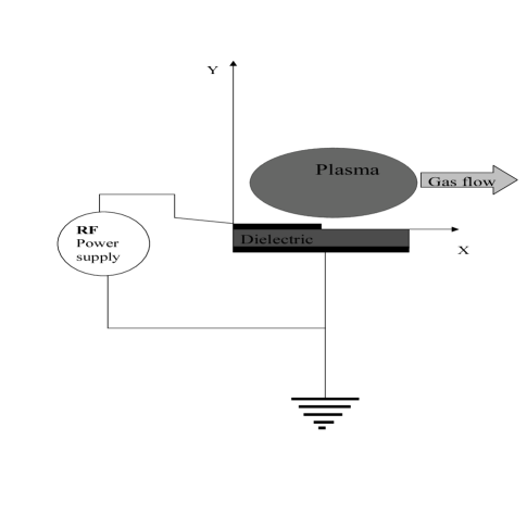
Figure 1: Schematic representation of electrode geometry of an energized OAUGDP plasma panel.

The simulation domain is a 2-DIM Cartesian geometry (see Fig. 1) with total length along the X-axis $L_{X}=0.4$ cm and height $L_{Y}=0.4$ cm; the width of the dielectric surface along the X-axis is 0.3 cm in Case Study I and 0.1 cm in Case Study II. The dielectric relative permittivity, supposed to be a ceramic material, is assumed to be $\varepsilon_{r}=100$; the dielectric thickness is in all cases set 0.065 cm. The capacity of the reactor is determined through the conventional formula $C_{ds}=\varepsilon_{0}\varepsilon_{r}S/d$. The electrodes thickness is supposed to be negligible.

II.2 Transport parameters and rate coefficients

The working gas is a ”airlike” mixture of a fixed fraction of nitrogen ($\delta_{N_{2}}=[N_{2}]/N=.78$) and oxygen ($\delta_{O_{2}}=[O_{2}]/N=0.22$), as is normally present at sea level at $p=1$ atm.

The electron homogeneous Boltzmann equation Ferreira is solved with the 2-term expansion in spherical harmonics for a mixture of $N_{2}-22\%$ O₂. The gas temperature is assumed constant both spatially and in time, $T_{g}=300$ K, and as well the vibrational temperature of nitrogen $T_{v}(N_{2})=2000$ K and oxygen $T_{v}(O_{2})=2000$ K. The set of cross sections of excitation by electron impact was taken from Siglo .

At atmospheric pressure the local equilibrium assumption holds: Transport coefficients ($\nu_{ion}^{N_{2}}$, $\nu_{ion}^{O_{2}}$, $\mu_{e}$, $\mu_{p}$, $D_{e}$, $D_{p}$) depend on space and time $(\textbf{r},t)$ only through the local value of the electric field $\mathbf{E}(\mathbf{r},t)$. This is the so called hydrodynamic regime.

Ion diffusion and mobility coefficients were taken from Sigmond , $\mu_{O_{2}^{-}}.N=6.85\times 10^{21}$ V^-1 m^-1 s^-1 (on the range of E/N with interest here), $\mu_{O_{2}^{+}}N=6.91\times 10^{21}$ V^-1 m^-1 s^-1, and $\mu_{N_{2}^{+}}N=5.37\times 10^{21}$ V^-1 m^-1 s^-1.

The reactions included in the present kinetic model are listed in Table  1. It is assumed that all volume ionization is due to electron-impact ionization from the ground state and the kinetic set consists basically in ionization, attachment and recombination processes. The kinetics of excited states and heavy neutral species is not considered.

To obtain a faster numerical solution of the present hydrodynamic problem it is assumed that the gas flow does not alter the plasma characteristics and is much smaller than the charged particle drift velocity. This assumption allows a simplified description of the flow. For more concise notation, we put $n_{p2}\equiv[N_{4}^{+}]$; $n_{p1}\equiv[N_{2}^{+}]$; $n_{p}\equiv[O_{2}^{+}]$; $n_{n}\equiv[O_{2}^{-}]$, and $n_{e}\equiv[e]$.

The balance equations for N${}_{4}^{+}$ (at atmospheric pressure the nitrogen ion predominant is N${}_{4}^{+}$) is:

$$\frac{\partial n_{p2}}{\partial t}+\mathbf{\nabla}\cdot(n_{p2}\mathbf{v}_{p2})=\delta_{N_{2}}^{2}N^{2}n_{p1}K_{ic1}-\beta Nn_{p2}-K_{r2}n_{p2}n_{e}.$$ (1)

The balance equation for N${}_{2}^{+}$ is:

$$\frac{\partial n_{p1}}{\partial t}+\mathbf{\nabla}\cdot(n_{p1}\mathbf{v}_{p2})=n_{e}\nu_{ion}^{N_{2}}+K_{ic2}[N_{2}]n_{p2}-\beta_{ii}n_{n}n_{p1}-\beta n_{e}n_{p1}-K_{ic1}[N_{2}]^{2}n_{p1}.$$ (2)

The oxygen ion considered is O${}_{2}^{+}$ and its resultant balance equation is given by

$$\frac{\partial n_{p}}{\partial t}+\mathbf{\nabla}\cdot(n_{p}\mathbf{v}_{p})=n_{e}\nu_{ion}^{O_{2}}-\beta_{ii}n_{n}n_{p}-\beta n_{e}n_{p}.$$ (3)

As oxygen is an attachment gas, the negative ion O${}_{2}^{-}$ was introduced and its balance equation was written as:

$$\frac{\partial n_{n}}{\partial t}+\mathbf{\nabla}\cdot(n_{n}\mathbf{v}_{n})=\nu_{att}^{O_{2}}n_{e}-\beta_{ii}n_{p1}n_{n}-K_{d}n_{p}n_{n}.$$ (4)

Finally, the balance equation for electrons can be written in the form:

$$\frac{\partial n_{e}}{\partial t}+\mathbf{\nabla}\cdot(n_{e}\mathbf{v}_{e})=n_{e}(\nu_{ion}^{N_{2}}+\nu_{ion}^{O_{2}}-\nu_{att}^{O_{2}})-\beta n_{e}(n_{p}+n_{p1})+K_{d}[O_{2}]n_{n}-K_{r2}n_{p1}n_{e}.$$ (5)

To close the above system of equations we use the drift-diffusion approximation for the charged particle mean velocities appearing in the continuity equations:

$$n_{i}\mathbf{v}_{i}=n_{i}\mu_{i}\mathbf{E}-\nabla(n_{i}D_{i}),$$ (6)

where $\mu_{i}$ and $D_{i}$ represent the charged particle mobility and the respective diffusion coefficient. The applied voltage has a sinusoidal wave form

$$V(t)=V_{dc}+V_{0}\sin(\omega t),$$ (7)

where $V_{dc}$ is the dc bias voltage (although here we fixed to ground, $V_{dc}=0$) and $\omega$ is the applied angular frequency. $V_{0}$ is the maximum amplitude with the root mean square voltage in this case of study $V_{rms}=5$ kV and the applied frequency $f=5$ kHz.

The total current (convective plus displacement current) was determined using the following equation given by Sato and Murray Sato

$$I_{d}(t)=\frac{e}{V}\int_{V}\left(n_{p}\mathbf{w}_{p}-n_{e}\mathbf{w}_{e}-n_{n}\mathbf{w}_{n}-D_{p}\frac{\partial n_{p}}{\partial z}+D_{e}\frac{\partial n_{e}}{\partial z}+D_{n}\frac{\partial n_{n}}{\partial z}\right)\cdot\mathbf{E}_{L}dv+\frac{\epsilon_{0}}{V}\int_{V}\left(\frac{\partial\mathbf{E}_{L}}{\partial t}\cdot\mathbf{E}_{L}\right)dv,$$ (8)

where $\int_{V}dv$ is the volume occupied by the discharge, $\mathbf{E}_{L}$ is the space-charge free component of the electric field. The last integral when applied to our geometry gives the displacement current component

$$I_{disp}(t)=\frac{\varepsilon_{0}}{d^{2}}\frac{\partial V}{\partial t}\int_{V}dv.$$ (9)

Auger electrons are assumed to be produced by impact of positive ions on the cathode with an efficiency $\gamma=5\times 10^{-2}$, so that the flux density of secondary electrons out of the cathode is given by

$$\mathbf{j}_{se}(t)=\gamma\mathbf{j}_{p}(t),$$ (10)

with $\mathbf{j}_{p}$ denoting the flux density of positive ions. In fact, this mechanism is of fundamental importance on the working of the OAUGDP^®.

Due to the accumulation of electric charges over the dielectric surface, a kind of ”memory voltage” is developed, whose expression is given by:

$$V_{m}(t)=\frac{1}{C_{ds}}\int_{t_{0}}^{t}I_{d}(t^{\prime})dt^{\prime}+V_{m}(t_{0}).$$ (11)

Here, $C_{ds}$ is the equivalent capacitance of the discharge.

The space-charge electric field was obtained by solving the Poisson equation

$$\Delta V=-\frac{e}{\epsilon_{0}}(n_{p}-n_{e}-n_{n}).$$ (12)

The boundary conditions are the following:

• electrode (Dirichlet boundary condition): $V(x,y=0,t)=V-V_{m}$;

• dielectric (Neumann boundary condition): $E_{n}=(\mathbf{E}\cdot\mathbf{n})=\frac{\sigma}{2\epsilon_{0}}$.

The flux of electric charges impinging on the dielectric surface builds up a surface charge density $\sigma$ which was calculated by balancing the flux to the dielectric

$$\frac{\partial\sigma}{\partial t}=e(|\Gamma_{p,n}|-|\Gamma_{e,n}|).$$ (13)

Here, $\mathbf{\Gamma}_{p,n}$ and $\mathbf{\Gamma}_{e,n}$ represent the normal component of the flux of positive and negative ions and electrons to the dielectric surface. Furthermore, it is assumed that ions and electrons recombine instantaneously on the perfectly absorbing surface.

The entire set of equations are solved together, at each time step, self-consistently.

Table 1: List of reactions taken into account in our model. Rate coefficients were taken from Ref. Kossyi92 .

kind of reaction	Process	Rate coefficient
Ionization	$e+N_{2}\to 2e+N_{2}^{+}$	$\nu_{ion}^{N_{2}}$
Ionization	$e+O_{2}\to 2e+O_{2}^{+}$	$\nu_{ion}^{O_{2}}$
3-body electron attachment	$e+O_{2}+O_{2}\to O_{2}^{-}+O_{2}$	$K_{a1}=1.4\times 10^{-29}(\frac{300}{T_{e}})\exp(-600/T_{g})K_{1}(T_{g},T_{e})$ (cm${}^{6}/$s)
3-body electron attachment	$e+O_{2}+N_{2}\to O_{2}^{-}+N_{2}$	$K_{a2}=1.07\times 10^{-31}(\frac{300}{T_{e}})^{2}K_{2}(T_{g},T_{e})$ (cm${}^{6}/$s)
Collisional detachment	$O_{2}^{-}+O_{2}\to e+2O_{2}$	$K_{d}=2.7\times 10^{-10}\sqrt{\frac{T_{g}}{300}}\exp(-5590/T_{g})$ (cm${}^{3}/$s)
e-ion dissociative recombination	$N_{2}^{+}+e\to 2N$	$\beta=2.8\times 10^{-7}\sqrt{\frac{300}{T_{g}}}$ (cm${}^{3}/$s)
e-ion dissociative recombination	$O_{2}^{+}+e\to 2O$	$\beta=2.8\times 10^{-7}\sqrt{\frac{300}{T_{g}}}$ (cm${}^{3}/$s)
2-body ion-ion recombination	$O_{2}^{-}+N_{2}^{+}\to O_{2}+N_{2}$	$\beta_{ii}=2\times 10^{-7}\sqrt{\frac{300}{T_{g}}}[1+10^{-19}N(\frac{300}{T_{g}})^{2}]$ (cm${}^{3}/$s)
Ion-conversion	$N_{2}^{+}+N_{2}+N_{2}\to N_{4}^{+}+e$	$K_{ic1}=5\times 10^{-29}$ (cm${}^{6}/$s)
Recombination	$N_{4}^{+}+e\to 2N_{2}$	$K_{r2}=2.3\times 10^{-6}/(Te/300)^{0.56}$
Ion-conversion	$N_{4}^{+}+N_{2}\to N_{2}^{+}+2N_{2}$	$K_{ic2}=2.1\times 10^{-16}\exp(T_{g}/121)$ (cm${}^{3}/$s)

III Method of resolution of fluid equations

The particle’s governing equations are of convection-diffusion type. They are solved using a method proposed by Patankar Patankar (see also Ref. Pinhao ). According to this method, let $L(\phi,d\phi,d^{2}\phi,...)=S$ be a homogeneous differential equation in $\phi$, with a source term $S$. Then the procedure of Patankar consists in replacing $L(\phi,d\phi,d^{2}\phi,...)=S$ by $a_{P}\phi_{P}=\sum_{k}a_{k}\phi_{k}+b$, where P is the central point of the mesh.

The chosen time step is limited by the value of the dielectric relaxation time. For the present calculations the total number of computational meshes used is (100x100). This fair condition allows calculating an entire cycle with an Intel Pentium 4 (2.66 GHz) in a reasonable CPU time of about 30 hours per cycle, limiting to a reasonable value the relative error $|\Delta w_{e}/w_{e}|$, with $w_{e}$ designating the electron drift velocity. Stationarity was attained typically after 4-5 cycles. Equations 1- 13 are integrated successively in time supposing the electric field is constant during each time step, obtaining a new value of the electric field after the end of each time step. The method used to integrate the continuity equations and Poisson equation was assured to be numerically stable, constraining the time step width to the well known Courant-Levy-Friedrich stability criterion.

IV Results

The simulations were done for a two-dimensional flat staggered geometry, as sketched in Fig. 1. This is essentially a ’surface discharge’ arrangement with asymmetric electrodes. It is assumed that the plasma is homogeneous along the OZ axis.

IV.1 Electrical characteristics

In Fig. 2 it is given the evolution along a period of time of the calculated electric current, applied voltage, gas voltage and memory voltage. The OAUGDP^®, and as well generically a DBD, occurs in configurations characterized by a dielectric layer between conducting electrodes. At about $740$ Volts, electron avalanches develop, replenishing the volume above the surface with charged particles. Hence, the charged particles are flowing to the dielectric (see Eq. 13) start accumulating on the surface, and build-up an electric field that prevents the occurrence of a high current, and quenches the discharge development at an early stage.

Figure 2: Electric current, applied voltage, gas voltage and memory voltage as a function of time. Conditions: Case I. Solid curve: current; dot curve: $V_{m}$; dashed-dot curve: $V_{g}$; dashed curve: $V$.

IV.2 Electrical field and potential

Fig. 3 shows the electric field during the first half-cycle at the instant of time $t=1.9\times 10^{-5}$ s. The energized electrode is the anode and the electric field follows Aston’s law, its magnitude remaining on the order of $10^{5}$ V$/$cm at a height of $8\times 10^{-5}$ m above the electrode and attaining lower magnitude above the dielectric surface, typically on the order of $10^{3}$ V$/$cm. The electric field magnitude is strongest in region around the inner edges of the energized electrode and dielectric surface (which is playing during this half-cycle the role of a pseudo-cathode).

During the avalanche development a strong ion sheath appears. In fact, as the avalanche develops an ion sheath expands along the dielectric surface until it reaches the boundary. With the ion sheath travels an electric field wave, with some similarities with a solitary wave. The speed of its propagation in the conditions of Fig. 3 is about 150 m$/$s. See Refs. Shyy ; Boeuf1 for very elucidating explanation of this phenomena.

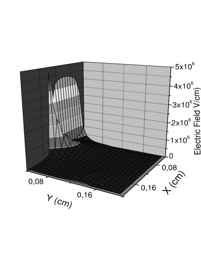
Figure 3: Electric field along OX and OY near the energized electrode at time $t=1.9\times 10^{-5}$ s at first half-cycle. Conditions: Case study I, with $V=5$ kV, $f=5$ kHz.

IV.3 Paraelectric gas flow control

The theory of paraelectric gas flow control was developed by Roth Roth1 . The electrostatic ponderomotive force $\mathbf{F_{E}}$ (units N$/$m³) acting on a plasma with a net charge density $\rho$ (units C$/$m³) is given by the electrostatic ponderomotive force and can be expressed under the form

$$\mathbf{F_{E}}=\frac{1}{2}\varepsilon_{0}\nabla E^{2}.$$ (14)

In order to verify whether electrostriction effects could be playing any significant role, it was also calculated the electrostriction ponderomotive force

$$\mathbf{F_{es}}=-\frac{1}{2}\varepsilon_{0}E^{2}\nabla\varepsilon_{r}.$$ (15)

Here, $\varepsilon_{r}=1-\frac{\omega_{p}^{2}}{\nu_{en}^{2}+\omega^{2}}$ is the relative permittivity of the plasma, $\nu_{en}$ is the electron-neutral momentum transfer frequency and $\omega_{p}$ is the plasma frequency. We found that this force term is negligible, contributing at maximum with 1 $\%$ to the total ponderomotive force. Subsequently, the ponderomotive forces were averaged over the area of calculation. Comparing the calculated space averaged ponderomotive forces per unit volume shown in Figs. 4- 5 it is seen that when the electrode width increases they become one order of magnitude higher. On average, during the second half-cycle the ponderomotive force magnitude decreases. This happens when the voltage polarity is reversed and the energized electrode play the role of cathode. This is due to a reduction of the potential gradient on the edge of the expanding plasma (see also Ref. Boeuf1 ). Calculations of EHD ponderomotive force have shown that its maximum intensity is attained during electron avalanches, with typical values on the order of $5\times 10^{9}$ N$/$m³. $\overline{F}_{x}$ points along OX (propelling direction), while $\overline{F}_{y}$ points downwards (boundary layer control).

Figure 4: Calculated space averaged ponderomotive forces per unit volume as a function of time. Solid curve: $F_{x}$; dot curve: $F_{y}$. Case study I

Figure 5: Calculated space averaged ponderomotive forces per unit volume as a function of time. Solid curve: $F_{x}$; dot curve: $F_{y}$. Case study II

IV.4 Gas speed

Using Bernoulli law (see Ref. Roth1 ) it can be obtained the induced neutral gas speed

$$v_{0}=E\sqrt{\frac{\varepsilon_{0}}{\rho}}=\sqrt{\frac{2}{\rho}\overline{F}_{x}L_{X}}.$$ (16)

Here, $\overline{F}_{x}$ is the calculated space average ponderomotive forces per unit volume, and $\rho=1.293$ Kg$/$m³. Fig. 6 shows the gas speed along the entire cycle in Case I. The average value of the gas speed is around 15 m$/$s while the experimental value, measured with a Pitot tube 1-2 mm above the surface, is 5 m$/$s as high as is for nearly the same operational conditions Roth04 .

Figure 6: Space averaged gas speed as a function of time. The straight solid line is a linear fit showing the increase of gas speed with time. Case I

Figure 7: Space averaged gas speed as a function of time. Case II

As can be seen in Fig. 7 the gas speed increases to about 20 m$/$s when the dielectric surface decreases. It is clear the slight decrease of the gas speed during the cathode cycle. This is related to the decrease of ponderomotive forces, as discussed above. As we assumed charged particles are totally absorbed on the dielectric surface, the swarm of ions propagating along the dielectric surface are progressively depleted, dwindle with time. However, it is worth to mentioning (see also Ref. Khudik ) that in certain conditions the inverse phenomena can happen, a bigger dielectric width feeding up the ion swarm with newborn ions and thus inducing an increase of the gas speed. How long its width can be increased is a matter of further study.

V Conclusion

A 2-DIM self-consistent kinetic model has been implemented to describe the electrical and kinetic properties of the OAUGDP^®. It was confirmed that the electric field follows the Aston’s law above the energized electrode. EHD ponderomotive forces on the order of $5\times 10^{9}$ N$/$m³ can be generated locally during the electron avalanches, their intensity decreasing afterwards to values well below on the order of $10^{4}\div 10^{5}$ N$/$m³. On the cathode side the EHD ponderomotive forces can decrease $1.5\div 2$ orders of magnitude, due probably to a smaller important potential gradient. The ponderomotive forces (and as well the gas speed) tend to increase whenever the energized electrode width augments relatively to the dielectric width.

This code will help to design an advanced propulsion system, achieving flow control in boundary layers and over airfoils by EHD means, with numerous advantages over conventional systems.

References

- (1) J. R. Roth, Physics of Plasmas 2003 10 2117
- (2) C. Liu, J. R. Roth, Paper 1P-26, Proceedings of the 21st IEEE International Conference on Plasma Science, Santa Fe, NM, June 6-8 1994, ISBN 7803-2006-9, pp. 97-98
- (3) J. R. Roth, D. M. Sherman, and S. P. Wilkinson, AIAA Journal 2000 38 1166
- (4) J. R. Roth, P. P.-Y. Tsai, C. Liu, M. Laroussi, and P. D. Spence, ”One Atmosphere Uniform Glow Discharge Plasma”, U. S. Patent 5414324, Issue May 9 (1995)
- (5) Roth, J R, Industrial Plasma Engineering, Vol.1: Principles (Bristol,IOP,1995)
- (6) Roth, J R, Industrial Plasma Engineering, Vol. 2: Application to Nonthermal Plasma Processing (Bristol,IOP,2001)
- (7) P. Bletzinger, B. N. Ganguly, D. Van Wie and A. Garscadden, J. Phys. D: Appl. Phys. 2005 38 R33-R57
- (8) Alfredo Soldati, Sanjoy Banerjee, Phys. Fluids 1998 10 1742
- (9) W. Shyy, B. Jayaraman, and A. Andersson, J. Appl. Phys. 2002 92 6434
- (10) Jérôme Pons, Eric Moreau and Gérard Touchard, J. Phys. D: Appl. Phys. 2005 38 3635
- (11) Zhiyu Chen, IEEE Trans. Plasma Sci. 2003 31 511
- (12) J. Reece Roth, R. C. M. Mohan, Manish Yadav, Jozef Rahel and, Stephen P. Wilkinson, AIAA Paper 2004-0845
- (13) R. B. Gadri, IEEE Trans. Plasma Sci. 1999 27 36
- (14) C. M. Ferreira, L. L. Alves, M. Pinheiro, and P. A. Sá, IEEE Trans. Plasma Sci. 1991 19 229
- (15) Siglo Data Base: http:cpat.ups-tlse.fr
- (16) R. S. Sigmond, Gas Discharge Data Sets for Dry Oxygen and Air , Electron and Ion Physics Research Group Report, the Norwegian Institute of Technology, The University of Trondheim (1979)
- (17) Kossyi I A, Kostinsky A Yu, Matveyev A A, and Silakov V P, Plasma Sources Sci. Technol. 1992 1 207
- (18) R. Morrow and N. Sato, J. Phys. D: Appl. Phys. 1999 32 L20-L22
- (19) S. V. Patankar, Numerical heat transfer and fluid flow, (New York: Taylor Francis,1980)
- (20) N. Pinhão, Modeling of the Discharge in Halogen Quenched Geiger-Muller Detectors (in Portuguese), Ph.D Thesis, Technical University of Lisbon, 1997
- (21) J. P. Boeuf and L. C. Pitchford, J. Appl. Phys. 2005 97 103307
- (22) A. Shvydky, V. P. Nagorny and V. N. Khudik, J. Phys. D: Appl. Phys. 2004 37 2996