Practicable factorized TDLDA for arbitrary density- and current-dependent functionals

Abstract

We propose a practicable method for describing linear dynamics of different finite Fermi systems. The method is based on a general self-consistent procedure for factorization of the two-body residual interaction. It is relevant for diverse density- and current-dependent functionals and, in fact, represents the self-consistent separable random-phase approximation (RPA), hence the name SRPA. SRPA allows to avoid diagonalization of high-rank RPA matrices and thus dwarfs the calculation expense. Besides, SRPA expressions have a transparent analytical form and so the method is very convenient for the analysis and treatment of the obtained results. SRPA demonstrates high numerical accuracy. It is very general and can be applied to diverse systems. Two very different cases, the Kohn-Sham functional for atomic clusters and Skyrme functional for atomic nuclei, are considered in detail as particular examples. SRPA treats both time-even and time-odd dynamical variables and, in this connection, we discuss the origin and properties of time-odd currents and densities in initial functionals. Finally, SRPA is compared with other self-consistent approaches for the excited states, including the coupled-cluster method.

I Introduction

The time-dependent local-density-approximation theory (TDLDA) is widely used for description of dynamics of diverse quantum systems such as atomic nuclei, atoms and molecules, atomic clusters, etc. (see for more details Row_70 ; Ring_Schuck_80 ; Dreizler_90 ; Bertsch_Broglia_94 ; Rein_Suraud_03 ). However, even in the linear regime, this theory is plagued by dealing with high-rank matrices which make the computational effort too expensive. This is especially the case for non-spherical systems with their demanding configuration space. For example, in the Random Phase Approximation (RPA), a typical TDLDA theory for linear dynamics, the rank of the matrices is determined by the size of the particle-hole 1ph space which becomes really huge for deformed and heavy spherical systems. The simplest RPA versions, like the sum rule approach and local RPA (see hierarchy of RPA methods in Rein_AP_92 ) deal with a few collective variables instead of a full 1ph space and thus avoid the problem of high-rank matrices. But these versions cannot properly describe gross-structure of collective modes and the related property of the Landau damping (dissipation of the collective motion over nearby 1ph excitations).

In this connection, we propose a method Ne_PRA_98 ; Ne_AP_02 ; Miori_01 ; Ne_PRC_1d which combines accuracy and power of involved RPA versions with simplicity and physical transparency of the simplest ones and thus is a good compromise between these two extremes. The method is based on the self-consistent separable approximation for the two-body residual interaction which is factorized into a sum of weighted products of one-body operators. Hence the method is called as separable RPA (SRPA). It should be emphasized that the factorization is self-consistent and thus does not result in any additional parameters. Expressions for the one-body operators and their weights are inambiguously derived from the initial functional. The factorization has the advantage to shrink dramatically the rank of RPA matrix (usually from $r=10^{3}-10^{6}$ to $r=2-14$) and thus to minimize the calculation expense. Rank of SRPA matrix is determined by the number of the separable terms in the expansion for the two-body interaction. Due to effective self-consistent procedure, usually a few separable terms (or even one term) are enough for a good accuracy. Ability of SRPA to minimize the computational effort becomes really decisive in the case of non-spherical systems with its huge 1ph configuration space. SRPA formalism is quite simple and physically transparent, which makes the method very convenient for the analysis and treatment of the numerical results. Being self-consistent, SRPA allows to extract spurious admixtures connected with violation of the translational or rotational invariance. As is shown below, SRPA exhibits accuracy of most involved RPA versions but for the much less expense. Since SRPA exploits the full 1ph space, it equally well treats collective and non-collective states and, what is very important, fully describes the Landau damping, one of the most important properties of collective motion. SRPA is quite general and can be applied to diverse finite Fermi systems (and thus to different functionals), including those tackling both time-even densities and time-odd currents. The latter is important not only for nuclear Skyrme functionals Skyrme ; Engel_75 which exploits a variety of time-even and time-odd variables but also for electronic functionals whose generalized versions deal with basic current densities (see e.g. KS_current ).

SRPA has been already applied for atomic nuclei and clusters, both spherical and deformed. To study dynamics of valence electrons in atomic clusters, the Konh-Sham functional KS ; GL was exploited Ne_PRA_98 ; Ne_AP_02 ; Ne_EPJD_98 ; Ne_EPJD_02 , in some cases together with pseudopotential and pseudo-Hamiltonian schemes Ne_EPJD_98 . Excellent agreement with the experimental data HS_99 for the dipole plasmon was obtained. Quite recently SRPA was used to demonstrate a non-trivial interplay between Landau fragmentation, deformation splitting and shape isomers in forming a profile of the dipole plasmon in deformed clusters Ne_EPJD_02 .

In atomic nuclei, SRPA was derived Miori_01 ; Ne_PRC_1d ; Prague_02 for the demanding Skyrme functional involving a variety of densities and currents (see Ben_RMP_03 for the recent review on Skyrme forces). SRPA calculations for isoscalar and isovector giant resonances (nuclear counterparts of electronic plasmons) in doubly magic nuclei demonstrated high accuracy of the method Ne_PRC_1d .

In the present paper, we give a detail, maybe even tutorial, description of SRPA, consider and discuss its most important particular cases and compare it with alternative approaches, including the equation-of-motion method in the coupled-cluster theory. We thus pursue the aim to advocate SRPA for researchers from other areas, e.g. from the quantum chemistry.

The paper is organized as follows. In Section II, derivation of the the SRPA formalism is done. Relations of SRPA with other alternative approaches are commented. In Sec. 3, the method to calculate SRPA strength function (counterpart of the linear response theory) is outlined. In Section IV, the particular SRPA versions for the electronic Kohn-Sham and nuclear Skyrme functionals are specified and the origin and role of time-odd currents in functionals are scrutinized. In Sec. V, the practical SRPA realization is discussed. Some examples demonstrating accuracy of the method in atomic clusters and nuclei are presented. The summary is done in Sec. VI. In Appendix A, densities and currents for Skyrme functional are listed. In Appendix B, the optimal ways to calculate SRPA basic values are discussed.

II Basic SRPA equations

RPA problem becomes much simpler if the residual two-body interaction is factorized (reduced to a separable form)

$$\sum_{h_{1},h_{2},p_{1},p_{2}}\!\!\!<h_{2}p_{2}|\hat{V}_{res}|p_{1}h_{1}>a^{+}_{p_{1}}a^{+}_{p_{2}}a_{h_{2}}a_{h_{1}}\rightarrow\sum_{k,k^{\prime}=1}^{K}[\kappa_{kk^{\prime}}{\hat{X}}_{k}{\hat{X}}_{k^{\prime}}+\eta_{kk^{\prime}}{\hat{Y}}_{k}{\hat{Y}}_{k^{\prime}}]$$ (1)

where

$${\hat{X}}_{k}=\sum_{ph}<p|{\hat{X}}_{k}|h>a^{+}_{p}a_{h},\quad{\hat{Y}}_{k}=\sum_{ph}<p|{\hat{Y}}_{k}|h>a^{+}_{p}a_{h}$$

are time-even and time-odd one-body operators, respectively. Further, $a^{+}_{p}$ ($a_{h}$) is the creation (annihilation) operator of the particle state $p$ (hole state $h$); $K$ is the number of the separable terms.

Conceptually, the self-consistent procedure outlined below was first proposed in LS_nuclei .

II.1 Time-dependent Hamiltonian

The system is assumed to undergo small-amplitude harmonic vibrations around HF ground state. The starting point is a general time-dependent energy functional

$$E(J_{\alpha}({\vec{r}},t))=\int{\cal H}(J_{\alpha}({\vec{r}},t))d{\vec{r}}$$ (2)

depending on an arbitrary set of densities and currents defined through the corresponding operators as

$$J_{\alpha}({\vec{r}},t)=<\Psi(t)|\hat{J}_{\alpha}({\vec{r}})|\Psi(t)>=\sum_{h}^{occ}\varphi^{*}_{h}({\vec{r}},t)\hat{J}_{\alpha}({\vec{r}})\varphi_{h}^{\mbox{}}({\vec{r}},t)$$ (3)

where $\Psi(t)$ is the many-body function of the system as a Slater determinant, and $\varphi^{*}_{h}$ is the wave function of the hole (occupied) single-particle state. In general, the set (3) includes both time-even and time-odd densities and currents, see examples in the Appendix A.

Time-dependent mean-field Hamiltonian directly follows from (2)-(3):

$$\hat{h}(\vec{r},t)\varphi_{h}=\frac{\delta{\cal H}}{\delta\varphi^{*}_{h}}=\sum_{\alpha}\frac{\delta{\cal H}}{\delta J_{\alpha}}\frac{\delta J_{\alpha}}{\delta\varphi^{*}_{h}}=\sum_{\alpha}\frac{\delta{\cal H}}{\delta J_{\alpha}}\hat{J}_{\alpha}\varphi_{h}.$$ (4)

In the small-amplitude regime, the densities are decomposed into static part and small time-dependent variation

$$J_{\alpha}({\vec{r}},t)=\bar{J}_{\alpha}({\vec{r}})+\delta J_{\alpha}({\vec{r}},t).$$ (5)

Then, to the linear order for $\delta J_{\alpha}({\vec{r}},t)$, the mean-field Hamiltonian (4) can be decomposed into static and time-dependent response parts

$$\hat{h}(\vec{r},t) = \hat{h}_{0}(\vec{r})+\hat{h}_{res}(\vec{r},t),$$ (6)

$$= \sum_{\alpha}[\frac{\delta{\cal H}}{\delta J_{\alpha}}]_{J=\bar{J}}{\hat{J}}_{\alpha}({\vec{r}})+\sum_{\alpha,\alpha^{\prime}}[\frac{\delta^{2}{\cal H}}{\delta J_{\alpha}\delta J_{\alpha^{\prime}}}]_{J=\bar{J}}\delta J_{\alpha^{\prime}}({\vec{r}},t){\hat{J}}_{\alpha}({\vec{r}})$$

and thus we get the time-dependent Hamiltonian $\hat{h}_{res}(\vec{r},t)$ responsible for the collective motion.

II.2 Scaling perturbation

Now we should specify the response Hamiltonian $\hat{h}_{res}(\vec{r},t)$. For this aim, we use the scaling transformation and define the perturbed many-body wave function of the system as

$$|\Psi(t)\!>=\prod_{k=1}^{K}exp[-iq_{k}(t)\hat{P}_{k}]exp[-ip_{k}(t)\hat{Q}_{k}]|0>.$$ (7)

Here both the perturbed wave function $|\Psi(t)\!>$ and static ground state wave function $|0>$ are Slater determinants; ${\hat{Q}}_{k}(\vec{r})$ and ${\hat{P}}_{k}(\vec{r})$ are generalized coordinate (time-even) and momentum (time-odd) hermitian operators with the propoerties.

$$\hat{Q}_{k}=\hat{Q}_{k}^{+},\quad\hat{T}\hat{Q}_{k}\hat{T}^{-1} = \hat{Q}_{k},$$

$$\hat{P}_{k}=i[\hat{H},\hat{Q}_{k}]_{ph}=\hat{P}_{k}^{+},\quad\hat{T}\hat{P}_{k}\hat{T}^{-1} = -\hat{P}_{k},\quad$$ (8)

They generate T-even and T-odd harmonic deformations $q_{k}(t)$ and $p_{k}(t)$; $\hat{T}$ is the time inversion operator.

Using Eqs. (3) and (7), the transition densities read

$$\delta J_{\alpha}({\vec{r}},t) =<\Psi(t)|{\hat{J}}_{\alpha}|\Psi(t)>-<0|{\hat{J}}_{\alpha}|0>=$$

$$=i\sum_{k}\{q_{k}(t)<0|[\hat{P}_{k},\hat{J}_{\alpha}(\vec{r})]|0>+p_{k}(t)<0|[\hat{Q}_{k},\hat{J}_{\alpha}(\vec{r})]|0>\}$$

and the response Hamiltonian (6) is

$$\hat{h}(\vec{r},t)=\sum_{sk}\{q_{k}(t)\hat{X}_{k}({\vec{r}})+p_{k}(t)\hat{Y}_{k}({\vec{r}})\}$$ (10)

where all the ${\vec{r}}$-dependent terms are collected into the hermitian one-body operators

$$\hat{X}_{k}({\vec{r}}) = i\sum_{\alpha\alpha^{\prime}}[\frac{\delta^{2}{\cal H}}{\delta J_{\alpha}\delta J_{\alpha^{\prime}}}]_{J=\bar{J}}<0|[\hat{P}_{k},{\hat{J}}_{\alpha^{\prime}}]|0>{\hat{J}}_{\alpha}(\vec{r}),$$ (11)

$$\hat{Y}_{k}({\vec{r}}) = i\sum_{\alpha\alpha^{\prime}}[\frac{\delta^{2}{\cal H}}{\delta J_{\alpha}\delta J_{\alpha^{\prime}}}]_{J=\bar{J}}<0|[\hat{Q}_{k},{\hat{J}}_{\alpha^{\prime}}]|0>{\hat{J}}_{\alpha}(\vec{r})$$ (12)

with the properties

$$\hat{X}_{k} = \hat{X}_{k}^{+},\quad T\hat{X}_{k}T^{-1}=\hat{X}_{k},\quad\hat{X}_{k}^{*}=\hat{X}_{k},$$ (13)

$$\hat{Y}_{k} = \hat{Y}_{k}^{+},\quad T\hat{Y}_{k}T^{-1}=-\hat{Y}_{k},\quad\hat{Y}_{k}^{*}=-\hat{Y}_{k}.$$ (14)

As is shown below, ${\hat{X}}_{k}$ and ${\hat{Y}}_{k}$ are just the T-even and T-odd operators to be exploited in the separable expansion (1).

In the derivation above, we used the property of hermitian operators with a definite T-parity

$$<0|[\hat{A},\hat{B}]|0>=0,\quad\mbox{if}\quad T\hat{A}T^{-1}=T\hat{B}T^{-1}$$ (15)

which states that the average of the commutator vanishes if the operators $\hat{A}$ and $\hat{B}$ are of the same T-parity. This property allows to classify operators with a definite T-parity in the SRPA formalism and thus to make the formalism simple and transparent. For example, in Eqs. (11)-(12), T-even and T-odd densities ${\hat{J}}_{\alpha}(\vec{r})$ contribute separately to ${\hat{X}}_{k}$ and ${\hat{Y}}_{k}$.

To complete the construction of the separable expansion (1), we should yet determine the strength matrices $\kappa_{kk^{\prime}}$ and $\eta_{kk^{\prime}}$. This can be done through variations of the basic operators

$$\delta{\hat{X}}_{k}(t) \equiv<\Psi(t)|{\hat{X}}_{k}|\Psi(t)>-<0|{\hat{X}}_{k}|0>=$$

$$=i\sum_{k^{\prime}}q_{k^{\prime}}(t)<0|[\hat{P}_{k^{\prime}},\hat{X}_{k}]|0>=-\sum_{k^{\prime}}q_{k^{\prime}}(t)\kappa_{k^{\prime}k}^{-1}\;,$$

$$\delta{\hat{Y}}_{k}(t) \equiv<\Psi(t)|{\hat{Y}}_{k}|\Psi(t)>-<0|{\hat{Y}}_{k}|0>=$$

$$=i\sum_{k^{\prime}}p_{k^{\prime}}(t)<0|[\hat{Q}_{k^{\prime}},\hat{Y}_{k}]|0>=-\sum_{k^{\prime}}p_{k^{\prime}}(t)\eta_{k^{\prime}k}^{-1}$$

where we introduce symmetric inverse strength matrices

$$\kappa_{k^{\prime}k}^{-1} =\kappa_{kk^{\prime}}^{-1}=-i<0|[\hat{P}_{k^{\prime}},{\hat{X}}_{k}]|0>=$$

$$=\int d{\vec{r}}\sum_{\alpha\alpha^{\prime}}[\frac{\delta^{2}{\cal H}}{\delta J_{\alpha^{\prime}}\delta J_{\alpha}}]<0|[\hat{P}_{k},{\hat{J}}_{\alpha}]|0><0|[\hat{P}_{k^{\prime}},{\hat{J}}_{\alpha^{\prime}}]|0>,$$

$$\eta_{k^{\prime}k}^{-1} =\eta_{kk^{\prime}}^{-1}=-i<0|[\hat{Q}_{k^{\prime}},{\hat{Y}}_{k}]|0>$$

$$=\int d{\vec{r}}\sum_{\alpha\alpha^{\prime}}[\frac{\delta^{2}{\cal H}}{\delta J_{\alpha^{\prime}}\delta J_{\alpha}}]<0|[\hat{Q}_{k},{\hat{J}}_{\alpha}]|0><0|[\hat{Q}_{k^{\prime}},{\hat{J}}_{\alpha^{\prime}}]|0>.$$

Then one gets

$$-\sum_{k}\kappa_{k^{\prime}k}\delta{\hat{X}}_{k}(t) = q_{k^{\prime}}(t),$$ (20)

$$-\sum_{sk}\eta_{k^{\prime}k}\delta{\hat{Y}}_{k}(t) = p_{k^{\prime}}(t)$$ (21)

and the response Hamiltonian (10) acquires the form

$$\hat{h}(\vec{r},t)=-\sum_{kk^{\prime}}\{\kappa_{kk^{\prime}}\delta\hat{X}_{k}(t)\hat{X}_{k^{\prime}}({\vec{r}})+\eta_{kk^{\prime}}\delta\hat{Y}_{k}(t)\hat{Y}_{k^{\prime}}({\vec{r}})\}.$$ (22)

Following Row_70 , the response Hamiltonian (22) leads to the same eigenvalue problem as the separable Hamiltonian

$${\hat{H}}_{RPA}={\hat{h}}_{0}+{\hat{V}}_{res},$$ (23)

with

$${\hat{V}}_{res}=-\frac{1}{2}\sum_{kk^{\prime}}[\kappa_{kk^{\prime}}{\hat{X}}_{k}{\hat{X}}_{k^{\prime}}+\eta_{kk^{\prime}}{\hat{Y}}_{k}{\hat{Y}}_{k^{\prime}}]$$ (24)

(see also discussion in the next subsections).

In principle, we already have in our disposal the SRPA formalism for description of the collective motion in space of collective variables. Indeed, Eqs. (11), (12), (II.2), and (II.2) deliver one-body operators and strength matrices we need for the separable expansion of the two-body interaction. The number K of the collective variables $q_{k}(t)$ and $p_{k}(t)$ and separable terms depends on how precisely we want to describe the collecive motion (see discussion in Section 4). For $K=1$, SRPA converges to the sum rule approach with a one collective mode Rein_AP_92 . For $K>1$, we have a system of K coupled oscillators and SRPA is reduced to the local RPA Re_PRA_90 ; Rein_AP_92 suitable for a rough description of several modes and or main gross-structure efects. However, SRPA is still not ready to describe the Landau fragmentation. For this aim, we should consider the detailed 1ph space. This will be done in the next subsection.

II.3 Introduction of 1ph space

Collective modes can be viewed as superpositions of 1ph configurations. It is convenient to define this relation by using the Thouless theorem which establishes the connection between two arbitrary Slater determinants Thouless . Then, the perturbed many-body wave function reads

$$|\Psi(t)>=(1+\sum_{ph}c_{ph}(t)\hat{A}^{+}_{ph})|\Psi_{0}>$$ (25)

where

$$\hat{A}^{+}_{ph}=a^{\dagger}_{p}a_{h}$$ (26)

is the creation operator of 1ph pair and

$$c_{ph}(t)=c^{+}_{ph}e^{i\omega t}+c^{-}_{ph}e^{-i\omega t}$$ (27)

is the harmonic time-dependent particle-hole amplitude. T-even $q_{k}(t)$ and T-odd $p_{k}(t)$ collective variables can be also specified as harmonic oscillations

$$q_{k}(t)=\bar{q}_{k}cos(\omega t)=\frac{1}{2}\bar{q}_{k}(e^{i\omega t}+e^{-i\omega t}),$$

$$p_{k}(t)=\bar{p}_{k}sin(\omega t)=\frac{1}{2i}\bar{p}_{k}(e^{i\omega t}-e^{-i\omega t}).$$ (28)

Substituting (10) and (25) into the time-dependent HF equation

$$i\frac{d}{dt}|\Psi(t)>=({\hat{h}}_{0}+{\hat{h}}_{res}(t))|\Psi(t)>,$$ (29)

one gets, in the linear approximation, the relation between $c^{\pm}_{ph}$ and collective deformations $\bar{q}_{k}$ and $\bar{p}_{k}$

$$c^{\pm}_{ph}=-\frac{1}{2}\frac{\sum_{k^{\prime}}[\bar{q}_{k^{\prime}}<ph|\hat{X}_{k^{\prime}}|0>\mp i\bar{p}_{k^{\prime}}<ph|\hat{Y}_{k^{\prime}}|0>]}{\varepsilon_{ph}\pm\omega},$$ (30)

where $\varepsilon_{ph}$ is the energy of 1ph pair.

In addition to Eqs. (II.2)-(II.2), the variations $\delta{\hat{X}}_{k}(t)$ and $\delta{\hat{Y}}_{k}(t)$ can be now obtained with the alternative perturbed wave function (25):

$$\delta{\hat{X}}_{k^{\prime}}(t) \!\!\!\!\!=\!\!\sum_{ph}(c_{ph}(t)^{*}<\!ph|\hat{X}_{k^{\prime}}|0\!>+c_{ph}(t)<\!0|\hat{X}_{k^{\prime}}|ph\!>),$$ (31)

$$\delta{\hat{Y}}_{k^{\prime}}(t) \!\!\!\!\!=\!\!\sum_{ph}(c_{ph}(t)^{*}<\!ph|\hat{Y}_{k^{\prime}}|0\!>+c^{s}_{ph}(t)<\!0|\hat{Y}_{k^{\prime}}|ph\!>).$$ (32)

It is natural to equate the dynamical variations of the basic operators $\delta{\hat{X}}_{k}$ and $\delta{\hat{Y}}_{k}$, obtained with the scaling (7) and Thouless (25) perturbed wave functions. This provides the additional relation between the amplitudes $c^{\pm}_{ph}$ and deformations $\bar{q}_{k}$ and $\bar{p}_{k}$ and finally result in the system of equations for the unknowns $\bar{q}_{k}$ and $\bar{p}_{k}$.

By equating (II.2)-(II.2) and (31)-(32) we get

$$-\sum_{k}q_{k}(t)\kappa_{kk^{\prime}}^{-1} = \sum_{ph}(c_{ph}(t)^{*}<\!ph|\hat{X}_{k^{\prime}}|0\!>+c_{ph}(t)<\!0|\hat{X}_{k^{\prime}}|ph\!>),$$ (33)

$$-\sum_{k}q_{k}(t)\eta_{kk^{\prime}}^{-1} = \sum_{ph}(c_{ph}(t)^{*}<\!ph|\hat{Y}_{k^{\prime}}|0\!>+c_{ph}(t)<\!0|\hat{Y}_{k^{\prime}}|ph\!>).$$ (34)

Substituting (27)-(30) into these expressions and collecting, for example, the terms at $e^{i\omega t}$, one finally gets

$$\sum_{k} \{\bar{q}_{k}[F_{k^{\prime}k}^{(XX)}-\kappa_{kk^{\prime}}^{-1}]+\bar{p}_{k}F_{k^{\prime}k}^{(XY)}\}=0,$$

$$\sum_{k} \{\bar{q}_{k}F_{k^{\prime}k}^{(YX)}+\bar{p}_{k}[F_{k^{\prime}k}^{(YY)}-\eta_{kk^{\prime}}^{-1}]\}=0$$ (35)

with

$$F_{k^{\prime}k}^{(XX)} =\sum_{ph}\frac{1}{\varepsilon_{ph}^{2}-\omega^{2}}\{<ph|\hat{X}_{k}|0>^{*}<ph|\hat{X}_{k^{\prime}}|0>(\varepsilon_{ph}+\omega)$$

$$\hskip 99.58464pt+<ph|\hat{X}_{k}|0><0|\hat{X}_{k^{\prime}}|ph>(\varepsilon_{ph}-\omega)\},$$

$$F_{k^{\prime}k}^{(YX)} =-i\sum_{ph}\frac{1}{\varepsilon_{ph}^{2}-\omega^{2}}\{<ph|\hat{Y}_{k}|0>^{*}<ph|\hat{X}_{k^{\prime}}|0>(\varepsilon_{ph}+\omega)$$

$$\hskip 99.58464pt+<ph|\hat{Y}_{k}|0><0|\hat{X}_{k^{\prime}}|ph>(\varepsilon_{ph}-\omega)\},$$

$$F_{k^{\prime}k}^{(XY)} =i\sum_{ph}\frac{1}{\varepsilon_{ph}^{2}-\omega^{2}}\{<ph|\hat{X}_{k}|0>^{*}<ph|\hat{Y}_{k^{\prime}}|0>(\varepsilon_{ph}+\omega)$$

$$\hskip 99.58464pt+<ph|\hat{X}_{k}|h><0|\hat{Y}_{k^{\prime}}|ph>(\varepsilon_{ph}-\omega)\},$$

$$F_{k^{\prime}k}^{(YY)} =\sum_{ph}\frac{1}{\varepsilon_{ph}^{2}-\omega^{2}}\{<ph|\hat{Y}_{k}|0>^{*}<ph|\hat{Y}_{k^{\prime}}|0>(\varepsilon_{ph}+\omega)$$

$$\hskip 99.58464pt+<ph|\hat{Y}_{k}|0><0|\hat{Y}_{k^{\prime}}|ph>(\varepsilon_{ph}-\omega)\}.$$

Equating determinant of the system (II.3) to zero, we get the dispersion equation for RPA eigenvalues $\omega_{\nu}$.

II.4 Normalization condition

By definition, RPA operators of excited one-phonon states read

$$\hat{Q}^{+}_{\nu}=\frac{1}{2}\sum_{ph}\{c^{\nu-}_{ph}\hat{A}^{+}_{ph}-c^{\nu+}_{ph}\hat{A}_{ph}\}$$ (40)

and fulfill

$$[\hat{Q}_{\nu},\hat{Q}_{\nu^{\prime}}^{+}]=\delta_{\nu,\nu^{\prime}},\quad[\hat{Q}_{\nu}^{+},\hat{Q}_{\nu^{\prime}}^{+}]=[\hat{Q}_{\nu},\hat{Q}_{\nu^{\prime}}]=0,$$ (41)

where $\hat{A}^{+}_{ph}$ and $c^{\nu\pm}_{ph}$ are given by (26) and (30), respectively. In the quasiboson approximation for $\hat{A}^{+}_{ph}$, the normalization condition $[\hat{Q}_{\nu},\hat{Q}_{\nu}^{+}]=1$ results in the relation

$$\sum_{ph}\{(c^{\nu-}_{ph})^{2}-(c^{\nu+}_{ph})^{2}\}=2.$$ (42)

Using (30), it can be reformulated in terms of the RPA matrix coefficients (II.3)-(II.3):

$$\sum_{ph}\{(c^{\nu-}_{ph})^{2}-(c^{\nu+}_{ph})^{2}\}$$ (43)

$$=\sum_{kk^{\prime}}\frac{1}{4}\{\bar{q}^{\nu}_{k^{\prime}}\bar{q}^{\nu}_{\bar{k}}\frac{\partial F_{k^{\prime}k}^{(XX)}(\omega_{\nu})}{\partial\omega_{\nu}}+2\bar{q}^{\nu}_{k^{\prime}}\bar{p}^{\nu}_{\bar{k}}\frac{\partial F_{k^{\prime}k}^{(YX)}(\omega_{\nu})}{\partial\omega_{\nu}}+\bar{p}^{\nu}_{k^{\prime}}\bar{p}^{\nu}_{\bar{k}}\frac{\partial F_{k^{\prime}k}^{(YY)}(\omega_{\nu})}{\partial\omega_{\nu}}\}=2N_{\nu}.$$

The variables $\bar{q}^{\nu}_{k}$ and $\bar{p}^{\nu}_{k}$ should be finally normalized by the factor $1/\sqrt{N_{\nu}}$.

II.5 General discussion

Eqs. (11), (12), (II.2), (II.2), (30), (II.3)-(II.3), and (40)-(43) constitute the basic SRPA formalism. It is worth now to comment some essential points:
$\bullet$ One may show (e.g. by using a standard derivation of the matrix RPA) that the separable Hamiltonian (23)-(24) with (40) results in the SRPA equations (II.3)-(II.3) if to express unknowns $c^{\nu\pm}_{ph}$ through $\bar{q}_{\bar{k}}$ and $\bar{p}_{\bar{k}}$. Generally, RPA equations for unknowns $c^{\nu\pm}_{ph}$ require the RPA matrix of the high rank equal to size of the $1ph$ basis. The separable approximation allows to reformulate the RPA problem in terms of much more compact unknows $\bar{q}_{\bar{k}}$ and $\bar{p}_{\bar{k}}$ (see relation (30) and thus to minimize the computational effort. As is seen from (II.3), the rank of the SRPA matrix is equal to a double number $K$ of the separable operators and hence is low.
$\bullet$ The number of RPA eigen-states $\nu$ is equal to the number of the relevant $1ph$ configurations used in the calculations. In heavy nuclei and atomic clusters, this number ranges the interval $10^{3}$-$10^{6}$. For every RPA state $\nu$, Eq. (II.3) delivers a particular set of the amplitudes $\bar{q}^{\nu}_{sk}$ and $\bar{p}^{\nu}_{sk}$ which, following Eq. (30), self-consistently regulate relative contrubutions of different T-even and T-odd oscillating densities to the $\nu$-state.
$\bullet$ Eqs. (11), (12), (II.2), (II.2) relate the basic SRPA values with the starting functional and input operators $\hat{Q}_{k}$ and $\hat{P}_{k}$ by a simple and physically transparent way. This makes SRPA very convenient for the analysis and treatment of the obtained results.
$\bullet$ It is instructive to express the basic SRPA operators via the separable residual interaction (24):

$$\hat{X}_{k}=[\hat{V}_{res},\hat{P}_{k}]_{ph},\qquad\hat{Y}_{k}=[\hat{V}_{res},\hat{Q}_{k}]_{ph}$$ (44)

where the index $ph$ means the $1ph$ part of the operator. It is seen that the T-odd operator $\hat{P}_{k}$ retains the T-even part of $V_{res}$ to build $\hat{X}_{k}$. Vice versa, the commutator with the T-even operator $\hat{Q}_{k}$ keeps the T-odd part of $V_{res}$ to build $\hat{Y}_{k}$.
$\bullet$ Some of the SRPA values read as averaged commutators between T-odd and T-even operators. This allows to establish useful relations with other models. For example, (II.2), (II.2) and (44) give

$$\kappa_{k^{\prime}k}^{-1}=-i<0|[\hat{P}_{k^{\prime}},{\hat{X}}_{k}]|0>=-i<0|[\hat{P}_{k^{\prime}},[\hat{V}_{res},{\hat{P}}_{k}]]|0>,$$ (45)

$$\eta_{k^{\prime}k}^{-1}=-i<0|[\hat{Q}_{k^{\prime}},{\hat{Y}}_{k}]|0>=-i<0|[\hat{Q}_{k^{\prime}},[\hat{V}_{res},{\hat{Q}}_{k}]]|0>.$$ (46)

The similar double commutators but with the full Hamiltonian (instead of the residual interaction) correspond to $m_{3}$ and $m_{1}$ sum rules, respectively, and so represent the spring and inertia parameters Re_PRA_90 in the basis of collective generators $\hat{Q}_{k}$ and $\hat{P}_{k}$. This allows to establish the connection of the SRPA with the sum rule approach BLM_79 ; LS_89 and local RPA Re_PRA_90 .

Besides, the commutator form of SRPA values can considerably simplify their calculation (see discussion in the Appendix B).
$\bullet$ SRPA restores the conservation laws (e.g. translational invariance) violated by the static mean field. Indeed, let’s assume a symmetry mode with the generator $\hat{P}_{\rm sym}$. Then, to keep the conservation law $[\hat{H},\hat{P}_{\rm sym}]=0$, we simply have to include $\hat{P}_{\rm sym}$ into the set of the input generators $\hat{P}_{k}$ together with its complement $\hat{Q}_{\rm sym}=i[\hat{H},\hat{P}_{\rm sym}]$.
$\bullet$ SRPA equations are very general and can be applied to diverse systems (atomic nuclei, atomic clusters, etc.) described by density and current-dependent functionals. Even Bose systems can be covered if to redefine the many-body wave function (25) exhibiting the perturbation through the elementary excitations. In this case, the Slater deterninant for 1ph excitations should be replaced by a perturbed many-body function in terms of elementary bosonic excitations.
$\bullet$ In fact, SRPA is the first TDLDA iteration with the initial wave function (7). A single iteration is generally not enough to get the complete convergence of TDLDA results. However, SRPA calculations demonstrate that high accuracy can be achieved even in this case if to ensure the optimal choice of the input operators $\hat{Q}_{k}$ and $\hat{P}_{k}$ and keep sufficient amount of the separable terms (see discussion in Sec. 5). In this case, the first iteration already gives quite accurate results.
$\bullet$ There are some alternative RPA schemes also delivering self-consistent factorization of the two-body residual interaction, see e.g. LS_nuclei ; SS ; Kubo ; Vor for atomic nuclei and YB_92 ; babst for atomic clusters. However, these schemes are usually not sufficiently general. Some of them are limited to analytic or simple numerical estimates LS_nuclei ; SS ; YB_92 , next ones start from phenomenological single-particle potentials and thus are not fully self-consistent Kubo , the others need a large number of the separable terms to get an appropriate numerical accuracy Vor ; babst . SRPA has evident advantages as compared with these schemes.
$\bullet$ After solution of the SRPA problem, the Hamiltonian (23)-(24) is reduced to a composition of one-phonon RPA excitations

$$\hat{H}=\sum_{\nu}\omega_{\nu}\hat{Q}^{+}_{\nu}\hat{Q}_{\nu}$$ (47)

where one-phonon operators are given by $(\ref{eq:Q_op})-(\ref{eq:Q_norm})$. Then, it is easy to get expressions of the equation-of-motion (EOM) method:

$$[\hat{H},\hat{Q}^{+}_{\nu}]=\omega_{\nu}\hat{Q}^{+}_{\nu},\quad[\hat{H},\hat{Q}_{\nu}]=-\omega_{\nu}\hat{Q}_{\nu}.$$ (48)

So, SRPA and EOM with the Hamiltonian (23)-(24) are equivalent. This allows to to establish the connection between the SRPA and couled-cluster EOM method with the single reference (see for reviews Barlett_99 ; Paldus_99 ; Piecuch_02 ; Piecuch_03 ). SRPA uses the excitation operators involving only singles (1ph) and so generally carries less correlations than EOM-CC. At the same time, SRPA delivers very elegant and physically transparent calculations scheme and, as is shown in our calculations, the correlations included to the SRPA are often quite enough to describe linear dynamics. It would be interesting to construct the approach combining advantages of SRPA and EOM-CC.

III Strength function

In study of response of a system to external fields, we are usually interested in the average strength function instead of the responses of particular RPA states. For example, giant resonances in heavy nuclei are formed by thousands of RPA states whose contributions in any case cannot be distinguished experimentally. In this case, it is reasonable to consider the averaged response described by the strength function. Besides, the calculation of the strength function is usually much easier.

For electric external fields of multipolarity $E\lambda\mu$, the strength function can be defined as

$$S_{L}(E\lambda\mu;\omega)=\sum_{\nu}\omega_{\nu}^{L}M_{\lambda\mu\nu}^{2}\zeta(\omega-\omega_{\nu})$$ (49)

where

$$\zeta(\omega-\omega_{j})=\frac{1}{2\pi}\frac{\Delta}{(\omega-\omega_{\nu})^{2}+(\Delta/2)^{2}}$$ (50)

is Lorentz weight with an averaging parameter $\Delta$ and

$$M_{\lambda\mu\nu}=\frac{1}{2}\sum_{ph}<ph|\hat{f}_{\lambda\mu}|0>(c^{\nu-}_{ph}+c^{\nu+}_{ph})\,$$ (51)

is the transition matrix element for the external field

$$\hat{f}_{\lambda\mu}=\frac{1}{1+\delta_{\mu,0}}r^{\lambda}(Y_{\lambda\mu}+Y^{{\dagger}}_{\lambda\mu}).$$ (52)

It is worth noting that, unlike the standard definition of the strength function with using $\delta(\omega-\omega_{\nu})$, we exploit here the Lorentz weight. It is very convenient to simulate various smoothing effects.

The explicite expression for (49) can be obtained by using the Cauchy residue theorem. For this aim, the strength function is recasted as a sum of $\nu$ residues for the poles $z=\pm\omega_{\nu}$. Since the sum of all the residues (covering all the poles) is zero, the residues with $z=\pm\omega_{\nu}$ (whose calculation is time consuming) can be replaced by the sum of residies with $z=\omega\pm i(\Delta/2)$ and $z=\pm\varepsilon_{ph}$ whose calculation is much less expensive (see details of the derivation in Ne_AP_02 ).

Finally, the strength function for L=0 and 1 reads as

$$S_{L}(E\lambda\mu,\omega) = \frac{1}{\pi}\Im\left[\frac{z^{L}\det|B(z)|}{\det|F(z)|}\right]_{z=\omega+i(\Delta/2)}$$

$$+ 2\sqrt{2}\sum_{ph}^{K_{p},K_{h}>0}\varepsilon_{ph}^{L}<ph|\hat{f}_{\lambda\mu}|0>^{2}\zeta(\omega-\varepsilon_{ph}).$$

The first term in (III) is contribution of the residual two-body interaction while the second term is the unperturbed (purely $1ph$) strength function. Further, $F(z)$ is determinant of the RPA symmetric matrix (II.3) of the rank $2K$, where $K$ is the number of the initial operators $\hat{Q_{k}}$. The symmetric matrix $B$ of the rank $(2K+1)$ is defined as

$$B_{nn^{\prime}}(z) = F_{nn^{\prime}}(z),$$ (54)

$$B_{2K+1,2K+1}(z) = 0,\quad B_{2K+1,n}(z)=B_{n,2K+1}(z)=A_{n}(z)$$

where $n,n^{\prime}=1,...,2K$ and left (right) indexes define lines (columns).

The values $A_{n}(z)$ read

$$A_{n=2k-1}^{(X)}(E\lambda\mu,z) = 4\sum_{ph}^{K_{p},K_{h}>0}\frac{\varepsilon_{ph}<ph|\hat{X}_{k}|0><ph|\hat{f}_{\lambda\mu}|0>}{\varepsilon_{ph}^{2}-z^{2}}$$ (55)

$$A_{n=2k}^{(Y)}(E\lambda\mu,z) = 4\sum_{ph}^{K_{p},K_{h}>0}\frac{z{<ph|\hat{Y}_{k}|0><ph|\hat{f}_{\lambda\mu}|0>}}{\varepsilon_{ph}^{2}-z^{2}}.$$

They form the right and low borders of the determinant $B$ thus fringering the RPA determinant $F$. The values $-A_{n}(z)$ in the most right column have the same indices as the corresponding strings of the RPA determinant. The values $A_{n}(z)$ in the lowest line have the same indices as the corresponding columns of the RPA determinant.

Derivation of the strentth function, given above, deviates from the standard one in the lineary response theory. Besides, the SRPA deals with the Lorentz weight instead of $\delta(\omega-\omega_{\nu})$ used in the linear response theory. At the same time, SRPA strength function and lineary response theory are conceptually the same approaches. Since the linear response theory is widely used in the coupled-cluster (CC) method, it would be interesting to consider the implementation of SRPA stength function method to CC. The linear response theory is widely used in the coupled-cluster (CC) method. In this connection, it would be interesting to enlarge the SRPA stength function method to CC.

IV Particular cases for clusters and nuclei

IV.1 Kohn-Sham functional for atomic clusters

Kohn-Sham functional for atomic clusters reads

$$E_{\rm tot}(t)=E_{\rm kin}(t)+E_{xc}(t)+E_{C}(t)=\int d{\vec{r}}{\cal H}(\rho({\vec{r}},t))$$ (56)

where

$$E_{\rm kin}(t) = \frac{\hbar^{2}}{2m_{e}}\int d{\vec{r}}\,\tau({\vec{r}},t)\;,$$ (57)

$$E_{xc}(t) = \int d{\vec{r}}\,\rho({\vec{r}},t)\,\epsilon_{xc}(\rho\left({\vec{r}},t)\right)\;,$$ (58)

$$E_{C}(t) = \frac{e^{2}}{2}\int\int d{\vec{r}}d{\vec{r}}_{1}\frac{(\rho({\vec{r}},t)-\rho_{i}({\vec{r}}))(\rho({\vec{r}}_{1},t)-\rho_{i}({\vec{r}}_{1}))}{|{\vec{r}}-{\vec{r}}_{1}|}$$ (59)

are kinetic, exchange-correlation (in the local density approximation), and Coulomb terms, respectively. Further, $\rho_{i}({\vec{r}})$ is the ionic density and $\rho({\vec{r}},t)$ and $\tau({\vec{r}},t)$ are density and kinetic energy density of valence electrons.

In atomic clusters, oscillations of valence electrons are generated by time-dependent variations of the electronic T-even density $\rho({\vec{r}},t)$ only. So, one may neglect in the SRPA formalism all T-odd densities and their variations $p_{k}(t)$. This makes SRPA equations especially simple. In particular, the density variation (II.2) is reduced to

$$\delta\rho({\vec{r}},t) =i\sum_{k}q_{k}(t)<0|[\hat{P}_{k},\hat{\rho}(\vec{r})]|0>$$

$$=-4i\sum_{k}q_{k}(t)\sum_{ph}^{K_{p},K_{h}>0}<ph|\hat{P_{k}}|0>\Re{<ph|\hat{\rho}|0>}$$

$$=i\sum_{k}q_{k}(t)\delta\rho({\vec{r}})$$

where

$$<ph|\hat{P}_{k}|0>=2i\varepsilon_{ph}<ph|\hat{Q}_{k}|>,$$ (61)

$$\delta\rho({\vec{r}})=-\frac{\hbar^{2}}{2m_{e}}({\vec{\bigtriangledown}}\bar{\rho}({\vec{r}})\cdot{\vec{\bigtriangledown}}Q_{k}({\vec{r}})+2\bar{\rho}({\vec{r}})\triangle Q_{k}({\vec{r}})).$$ (62)

Here, $\Re{<ph|\hat{\rho}|0>}$ is the transition density and $\bar{\rho}({\vec{r}})$ is the static ground state density of valence electrons.

It is seen from (IV.1)-(61) that there are two alternative ways to calculate the density variation: i) through the transition density and matrix elements of $\hat{Q}_{k}$-operator and ii) through the ground state density. The second way is the most simple. It becomes possible because, in atomic clusters, $V_{res}$ has no T-odd $\hat{Y}_{k}$-operators and thus the commutator of $\hat{Q}_{k}$ with the full Hamiltonian is reduced to the commutator with the kinetic energy term only:

$$\hat{P}_{k}=i[\hat{H},\hat{Q}_{k}]_{ph}=i[\hat{h}_{0},\hat{Q}_{k}]_{ph}=-i\frac{\hbar^{2}}{2m_{e}}[\vec{\bigtriangledown}^{2},\hat{Q}_{k}]_{ph}.$$ (63)

This drastically simplifies SRPA expressions and allows to present them in terms of the static ground state density. The scaling tranformation (7) loses exponents with $p_{k}(t)$ and reads

$$|\Psi(t)\!>=\prod_{k=1}^{K}exp\{-iq_{k}(t)\hat{P}_{k}\}|0>.$$ (64)

Other SRPA equations are reduced to

$$\hat{X}_{k}({\vec{r}}) = i[\frac{\delta^{2}{\cal H}}{\delta\rho\delta\rho}]_{\rho=\bar{\rho}}<0|[\hat{P}_{k},{\hat{\rho}}]|0>{\hat{\rho}}(\vec{r})$$ (65)

$$= (\frac{\partial^{2}{\cal H}_{xc}}{\partial\rho\partial\rho})_{\rho={\bar{\rho}}}\delta\rho({\vec{r}})+e^{2}\int d{\vec{r}}_{1}\frac{\delta\rho({\vec{r}}_{1})}{|{\vec{r}}-{\vec{r}_{1}}|},$$

$$\kappa_{k^{\prime}k}^{-1} =\kappa_{kk^{\prime}}^{-1}=-i<0|[\hat{P}_{k^{\prime}},{\hat{X}}_{k}]|0>$$ (66)

$$=\int d{\vec{r}}\{\frac{\delta^{2}{\cal H}}{\delta\rho\delta\rho}\}_{\rho={\bar{\rho}}}<0|[\hat{P}_{k},{\hat{\rho}}]|0><0|[\hat{P}_{k^{\prime}},{\hat{\rho}}]|0>$$

$$=-\int d{\vec{r}}X_{k}({\vec{r}})\delta\rho({\vec{r}}),$$

$$\sum_{k}\bar{q}_{k}^{\nu}\{F_{k^{\prime}k}^{(XX)}-\kappa_{kk^{\prime}}^{-1}]\}=0,$$ (67)

$$c^{\nu\pm}_{ph}=-\frac{1}{2}\frac{\sum_{k}\bar{q}_{k}^{\nu}<ph|\hat{X}_{k}|0>}{\varepsilon_{ph}\pm\omega_{\nu}},$$ (68)

$$\sum_{ph}\{(c^{\nu-}_{ph})^{2}-(c^{\nu+}_{ph})^{2}\}=\sum_{kk^{\prime}}\frac{1}{4}\bar{q}^{\nu}_{k}\bar{q}_{k^{\prime}}^{\nu}\frac{\partial F_{kk^{\prime}}^{(XX)}(\omega_{\nu})}{\partial\omega_{\nu}}=2N_{\nu}.$$ (69)

It is seen that the basic operator (65) and strength matrix (66) have now simple expressions via $\delta\rho({\vec{r}})$ from (62). The operator (65) has exchange-correlation and Coulomb terms. For electric multipole oscillations (dipole plasmon, …), the Coulomb term dominates.

In recent years, there appear some new functionals where the current of electrons instead of their density is used as a basic variable KS_current . SRPA equations for this case can be straightforwardly obtained from the general formalism given in Sec. 2.

IV.2 Skyrme functional for atomic nuclei

Nuclear interaction is very complicated and its explicit form is still unknown. So, in practice different approximations to nuclear interaction are used. Skyrme forces Skyrme ; Engel_75 represent one of the most successful approximations where the interaction is maximally simplified and, at the same time, allows to get accurate and universal description of both ground state properties and dynamics of atomic nuclei (see Ben_RMP_03 a for recent review). Skyrme forces are contact, i.e. $\sim\delta({\vec{r}}_{1}-{\vec{r}}_{2})$, which minimizes the computational effort. In spite of this dramatic simplification, Skyrme forcese well reproduce properties of most spherical and deformed nuclei as well as characteristics of nuclear matter and neutron stars. Additional advantage of the Skyrme interaction is that its parameters are directly related to the basic nuclear properties: incompressibility, nuclear radii, masses and binding energies, etc. SRPA for Skyrme forces was derived in Miori_01 ; Ne_PRC_1d ; Prague_02 ; LS .

Although Skyrme forces are relatively simple, they are still much more demanding than the Coulomb interaction. In particular, they deal with a variety of diverse densities and currents. The Skyrme functional reads Engel_75 ; Re_nucl_AP_92 ; Dob_PRC_95

$${E}=\int d{\vec{r}}\left({\cal H}_{\rm kin}+{\cal H}_{\rm Sk}(\rho_{s},\tau_{s},\vec{\sigma}_{s},\vec{j}_{s},\vec{J}_{s})+{\cal H}_{\rm C}(\rho_{p})\right),$$ (70)

where

$${\cal H}_{\rm kin} = \frac{\hbar^{2}}{2m}\tau,$$ (71)

$${\cal H}_{\rm C} = \frac{e^{2}}{2}\int d{\vec{r}}^{\prime}\rho_{p}(\vec{r})\frac{1}{|\vec{r}-\vec{r}^{\prime}|}\rho_{p}(\vec{r}^{\prime})-\frac{3}{4}e^{2}(\frac{3}{\pi})^{\frac{1}{3}}[\rho_{p}(\vec{r})]^{\frac{4}{3}},$$ (72)

$${\cal H}_{\rm Sk} = \frac{b_{0}}{2}\rho^{2}-\frac{b^{\prime}_{0}}{2}\sum_{s}\rho_{s}^{2}-\frac{b_{2}}{2}\rho\Delta\rho+\frac{b^{\prime}_{2}}{2}\sum_{s}\rho_{s}\Delta\rho_{s}$$

$$+\frac{b_{3}}{3}\rho^{\alpha+2}-\frac{b^{\prime}_{3}}{3}\rho^{\alpha}\sum_{s}\rho_{s}^{2}$$

$$+b_{1}(\rho\tau-\vec{j}^{2})-b^{\prime}_{1}\sum_{s}(\rho_{s}\tau_{s}-\vec{j}_{s}^{2})$$

$$-b_{4}\left(\rho\vec{\nabla}\vec{{\Im}}+\vec{\sigma}\cdot(\vec{\nabla}\times\vec{j})\right)-b^{\prime}_{4}\sum_{s}\left(\rho_{s}(\vec{\nabla}\vec{\Im}_{s})+\vec{\sigma}_{s}\cdot(\vec{\nabla}\times\vec{j}_{s})\right)$$

$$+\tilde{b}_{4}\left(\vec{\sigma}\vec{T}-\vec{\Im}^{2}\right)+\tilde{b}^{\prime}_{4}\sum_{s}\left(\vec{\sigma}_{s}\vec{T}_{s}-\vec{\Im}_{s}^{2}\right)$$

are kinetic, Coulomb and Skyrme terms respectively. The isospin index $s=n,p$ covers neutrons (n) and protons (p). Densities without this index involve both neutrons and protons, e.g. $\rho=\rho_{p}+\rho_{n}$. Parameters $b$ and $\alpha$ are fitted to describe ground state properties of atomic nuclei.

The functional includes diverse densities and currents, both neutrons and protons. They are naturally separated into two groups: 1) T-even density $\rho_{s}(\vec{r})$, kinetic energy density $\tau_{s}(\vec{r})$ and spin orbital density $\vec{\Im}_{s}(\vec{r})$ and 2) T-odd spin density $\sigma_{s}(\vec{r})$, current $\vec{j}_{s}(\vec{r})$ and vector kinetic energy density $\vec{T}_{s}(\vec{r})$. Explicit expressions for these densities and currents, as well as for their operators, are given in the appendix A. Only T-even densities contribute to the ground state properties of nuclei with even numbers of protons and neutrons (and thus with T-even wave function of the ground state). Instead, both T-even and T-odd densities participate in generation of nuclear oscillations. Sec. 2 delivers the SRPA formalism for this general case.

IV.3 T-odd densities and currents

Comparison of the Kohn-Sham and Skyrme functionals leads to a natural question why these two functionals exploit, for the time-dependent problem, so different sets of basic densities and currents? If the Kohn-Sham functional is content with one density, the Skyrme forces operate with a diverse set of densities and currents, both T-even and T-odd. Then, should we consider T-odd densities as genuine for the description of dynamics of finite many-body systems or they are a pequliarity of nuclear forces? This question is very nontrivial and still poorly studied. We present below some comments which, at least partly, clarify this point.

Actual nuclear forces are of a finite range. These are, for example, Gogny forces Gogny_75 representing more realistic approximation of actual nuclear forces than Skyrme approximation. Gogny interaction has no any velocity dependence and fulfills the Galilean invariance. Instead, two-body Skyrme interaction depends on relative velocities $\vec{k}=1/2i\cdot(\vec{\nabla}_{1}-\vec{\nabla}_{2})$, which just simulates the finite range effects Ben_RMP_03 .

The static Hartree-Fock problem assumes T-reversal invariance and T-even single-particle density matrix. In this case, Skyrme forces can be limited by only T-even densities: $\rho_{s}(\vec{r})$, $\tau_{s}(\vec{r})$ and $\vec{\Im}_{s}(\vec{r})$. In the case of dynamics, the density matrix is not already T-even and aquires T-odd components Engel_75 . This fact, together with velocity dependence of the Skyrme interaction, results in appearance in the Skyrme functional of T-odd densities and currents: $\vec{s}_{s}(\vec{r})$, $\vec{j}_{s}(\vec{r})$ and $\vec{T}_{s}(\vec{r})$ Engel_75 ; Re_nucl_AP_92 . Hence the origin of T-odd densities in the Skyrme functional. However, this is not the general case for nuclear forces.

As compared with the Kohn-Sham functional for electronic systems, the nuclear Skyrme functional is less genuine. The main (Coulomb) interaction in the Kohn-Sham problem is well known and only exchange and corellations should be modeled. Instead, in the nuclear case, even the basic interaction is unknown and should be approximated, e.g. by the simple contact interaction in Skyrme forces.

The crudeness of Skyrme forces has certain consequences. For example, the Skyrme functional has no any exchange-correlation term since the relevant effects are supposed to be already included into numerous Skyrme fitting parameters. Besides, the Skyrme functional may accept a diverse set of T-even and T-dd densities and currents. One may say that T-odd densities appear in the Skyrme functional partly because of its specific construction. Indeed, other effective nuclear forces (Gogny Gogny_75 , Landau-Migdal LM ) do not exploit T-odd densities and currents for description of nuclear dynamics.

Implementation of a variety of densities and currents in the Skyrme fuctional has, however, some advantages. It is known that different projectiles and external fields used to generate collective modes in nuclear reactions are often selective to particular densities and currents. For example, some elastic magnetic collective modes (scissors, twist) are associated with variations in the momentum space while keeping the common density $\rho_{s}(\vec{r})$ about constant. T-odd densities and currents can play here a significant role while Skyrme forces obtain the advantage to describe the collective motion by a natural and physically transparent way.

Relative contributions of T-odd densities to a given mode should obviously depend on the character of this mode. Electric multipole excitations (plasmons in atomic clusters, $E\lambda$ giant resonances in atomic nuclei) are mainly provided by T-even densities (see e.g. Prague_02 ). Instead, T-odd densities and currents might be important for magnetic modes and maybe some exotic (toroidal, …) electric modes.

It worth noting that T-odd denstities appear in the Skyrme functional in the specific combinations $\rho_{s}\tau_{s}-\vec{j}_{s}^{2}$, $\rho_{s}(\vec{\nabla}\vec{\Im}_{s})+\vec{\sigma}_{s}\cdot(\vec{\nabla}\times\vec{j}_{s})$, and $\vec{\sigma}_{s}\vec{T}_{s}-\vec{\Im}_{s}^{2}$. Following Dob_PRC_95 , this ensures Skyrme forces to fulfill the local gauge invariance (and Galilean invariance as the particular case). The velocity-independent finite-range Gogny forces also keep this invariance. Being combined into specific combinations, T-odd densities do not require any new Skyrme parameters Dob_PRC_95 . So, the parameters fitted to the static nuclear properties with T-even densities only, are enough for description of the dynamics as well.

The time-dependent density functional theory RG_84 for electronic systems is usually implemented at adiabatic local density approximation (ALDA) when density and single-particle potential are supposed to vary slowly both in time and space. Last years, the current-dependent Kohn-Sham functionals with a current density as a basic variable were introduced to treat the collective motion beyond ALDA (see e.g. KS_current ). These functionals are robust for a time-dependent linear response problem where the ordinary density functionals become strongly nonlocal. The theory is reformulated in terms of a vector potential for exchange and correlations, depending on the induced current density. So, T-odd variables appear in electronic functionals as well.

In general, the role of T-odd variables in dynamics of finite many-body systems is still rather vague. This fundamental problem devotes deep and comprehensive study.

V Choice of initial operators

It is easy to see that, after choosing the initial operators $\hat{Q}_{k}({\vec{r}})$, all other SRPA values can be straightforwardly determined following the steps

$$\hat{Q}_{k}\;\Rightarrow\;<|[\hat{Q}_{k},{\hat{J}}_{\alpha}]|>\;\Rightarrow\;\hat{Y}_{k},\;\eta_{kk^{\prime}}^{-1}\;\Rightarrow\;\hat{P}_{k}\;\Rightarrow\;<|[\hat{P}_{k},{\hat{J}}_{\alpha}]|>\;\Rightarrow\;\hat{X}_{k},\;\kappa_{kk^{\prime}}^{-1}.$$

As was mentioned above, the proper choice of initial operators $\hat{Q}_{k}({\vec{r}})$ is crucial to achieve good convergence of the separable expansion (1) with a minimal number of separable operators.

SRPA itself does not give a recipe to determine $\hat{Q}_{k}({\vec{r}})$. But choice of these operators can be inspired by physical and computational arguments. The operators should be simple and universal in the sense that they can be applied equally well to all modes and excitation channels. The main idea is that the initial operators should result in exploration of different spatial regions of the system, the surface and interior. This suggests that the leading scaling operator should have the form of the applied external field in the long-wave approximation, for example,

$$\hat{Q}^{\lambda\mu}_{k=1}({\vec{r}})=r^{\lambda}(Y_{\lambda\mu}(\Omega)+\mbox{h.c.)}.$$ (74)

Such a choice results in the separable operators (11), (12) and (65) most sensitive to the surface of the system. This is evident in (65) where $\delta\rho({\vec{r}})\propto{\vec{\bigtriangledown}}\bar{\rho}({\vec{r}})$ is peaked at the surface. Many collective oscillations manifest themselves as predominantly surface modes. As a result, already one separable term generating by (74) usually delivers a quite good description of collective excitations like plasmons in atomic clusters and giant resonances in atomic nuclei. The detailed distributions depends on a subtle interplay of surface and volume vibrations. This can be resolved by taking into account the nuclear interior. For this aim, the radial parts with larger powers $r^{\lambda+n_{k}}Y_{\lambda\mu}$ and spherical Bessel functions can be used, much similar as in the local RPA Re_PRA_90 . This results in the shift of the maxima of the operators (11), (12) and (65) to the interior. Exploring different conceivable combinations, one may found a most efficient set of the initial operators.

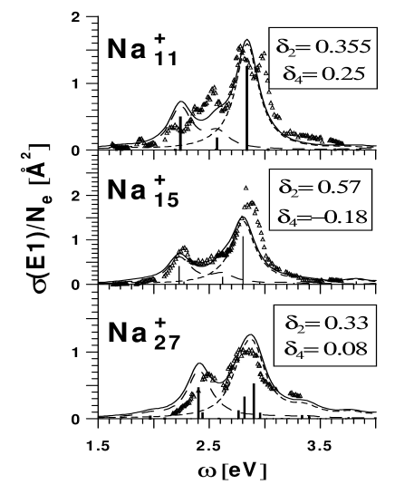
Figure 1: Photoabsorption cross section for the dipole plasmon in axially deformed sodium clusters, normalized to the number of valence electrons $N_{e}$. The parameters of quadrupole and hexadecapole deformations are given in boxes. The experimental data SH (triangles) are compared with SRPA results given as bars for RPA states and as the strength function (49) smoothed by the Lorentz weight with $\Delta=0.25$ eV. Contributions to the strength function from $\mu=$0 and 1 dipole modes (the latter has twice larger strength) are exhibited by dashed curves. The bars are given in $eV\AA^{2}$.

For description of the dipole plasmon in atomic clusters, the set of hermitian operators

$$Q^{\lambda_{k}\mu}_{k}({\vec{r}})=r^{\lambda_{k}+n_{k}}(Y_{\lambda_{k}\mu}(\Omega)+Y_{\lambda_{k}\mu}^{{\dagger}}(\Omega))$$ (75)

with $\lambda_{k}n_{k}$ = 10, 12, 14 and $\mu=0,1$ is usually enough Ne_AP_02 ; Ne_EPJD_02 . As is seen from Fig. 1, we successfully reproduce gross structure of the dipole plasmon in light axially-deformed sodium clusters (some discrepancies for the lightest cluster Na${}_{11}^{+}$ arise because of the roughness of the ionic jellium approximation for smallest samples). Already one initial operator is usually enough to reproduce the energy of the dipole plasmon and its branches but in this case the plasmon acquires some artificial strength in its right flank and thus the overestimated width Ne_PRA_98 . This problem can be solved by adding two more initial operators. The calculations for a variety of spherical alkali metal clusters Ne_EPJD_98 as well as for deformed clusters of a medium size Ne_EPJD_02 show that SRPA correcly describes not only gross structure of the dipole plasmon but also its Landau damping and width.

For the description of giant resonances in atomic nuclei, we used the set of initial operators Ne_PRC_1d

$$\hat{Q}_{k}({\vec{r}})=R_{k}(r)(Y_{\lambda\mu}(\Omega)+\mbox{h.c.})$$ (76)

with

$$R_{k}(r)=\left\{\begin{array}[]{ll}r^{\lambda},&k\!=\!1\\ j_{\lambda}(q^{k}_{\lambda}r),&k\!=\!2,3,4\\ \end{array}\right.$$ (77)

$$q^{k}_{\lambda}=a_{k}\frac{z_{\lambda}}{R_{\rm diff}},\quad a_{2}\!=\!0.6\;,a_{3}\!=\!0.9\;,a_{4}\!=\!1.2$$

where $R_{\rm diff}$ is the diffraction radius of the actual nucleus and $z_{\lambda}$ is the first root in of the spherical Bessel function $j_{\lambda}(z_{\lambda})=0$. The separable term with $k=1$ is mainly localized at the nuclear surface while the next terms are localized more and more in the interior. This simple set seems to be a best compromise for the description of nuclear giant resonances in light and heavy nuclei.

Figure 2: Isoscalar E2 and isovector E1 giant resonances in ${}^{40}Ca$ calculated with SkM* forces. The results are exhibited for full (exact) RPA (solid curve) and SRPA with $k=1$ (dotted curve).

Fig. 2 demonstrates that already one separable term (k=1) can be enough to get a reasonable agreement with the exact results. For k=1, the calculations are especially simple and results are easily analyzed.

The sets (75)-(77) are optimal for description of electric collective modes ($E\lambda$ plasmons in clusters and giant resonances in nuclei). For description of magnetic modes, the initial operator should resemble the T-odd magnetic external field. So, in this case we should start from the initial operators $\hat{P}_{k}$ in the form of the magnetic multipole transition operator in the long-wave approximation. The T-even operators $\hat{Q}_{k}$ are then obtained from the connection $\hat{Q}_{k}=i[\hat{H},\hat{P}_{k}]$.

VI Summary

We presented fully self-consistent separable random-phase-approximation (SRPA) method for description of linear dynamics of different finite Fermi-systems. The method is very general, physically transparent, convenient for the analysis and treatment of the results. SRPA drastically simplifies the calculations. It allows to get a high numerical accuracy with a minimal computational effort. The method is especially effective for systems with a number of particles $10-10^{3}$, where quantum-shell effects in the spectra and responses are significant. In such systems, the familiar macroscopic methods are too rough while the full-scale microscopic methods are too expensive. SRPA seems to be here the best compromise between quality of the results and the computational effort. As the most involved methods, SRPA describes the Landau damping, one of the most important characteristics of the collective motion. SRPA results can be obtained in terms of both separate RPA states and the strength function (linear response to external fields).

The particular SRPA versions for electronic Kohn-Sham and nuclear Skyrme functional were considered and examples of the calculations for the dipole plasmon in atomic clusters and giant resonances in atomic nuclei were presented. SRPA was compared with alternative methods, in particular with EOM-CC. It would be interesting to combine advantages of SRPA and couled-cluster approach in one powerful method.

Acknowledgments. The work was partly supported by the DFG grant (project GZ:436 RUS 17/104/05) and the grants Heisenberg-Landau (Germany - BLTP JINR) and Votruba-Blokhintcev (Czech Republic - BLTP JINR).

Appendix A: Densities and currents for Skyrme functional

In Skyrme forces, the complete set of the densities involves the ordinary density, kinetic-energy density, spin-orbital density, current density, spin density and vector kinetic-energy density:

$$\rho_{s}({\vec{r}},t) = \sum_{h\epsilon s}^{occ}\varphi^{*}_{h}({\vec{r}},t)\varphi_{h}^{\mbox{}}({\vec{r}},t),\qquad\qquad\qquad\qquad\qquad\qquad\quad\hat{T}\rho\hat{T}^{-1}=\rho$$

$$\tau_{s}({\vec{r}},t) = \sum_{h\epsilon s}^{occ}\vec{\nabla}\varphi^{*}_{h}({\vec{r}},t)\!\cdot\!\vec{\nabla}\varphi_{h}^{\mbox{}}({\vec{r}},t),\qquad\qquad\qquad\qquad\qquad\quad\hat{T}\tau\hat{T}^{-1}=\tau$$

$$\vec{\Im}_{s}({\vec{r}},t) = -i\sum_{h\epsilon s}^{occ}\varphi^{*}_{h}({\vec{r}},t)(\vec{\nabla}\times\hat{\vec{\sigma}})\varphi_{h}^{\mbox{}}({\vec{r}},t),\qquad\quad\qquad\qquad\quad\hat{T}{\vec{\Im}}\hat{T}^{-1}={\vec{\Im}}$$

$$\vec{j}_{s}({\vec{r}},t) = -\frac{i}{2}\sum_{h\epsilon s}^{occ}\left[\varphi^{*}_{h}({\vec{r}},t)\vec{\nabla}\varphi_{h}^{\mbox{}}({\vec{r}},t)-\vec{\nabla}\varphi^{*}_{h}({\vec{r}},t)\varphi_{h}^{\mbox{}}({\vec{r}},t)\right],\quad\hat{T}{\vec{j}}\hat{T}^{-1}=-{\vec{j}}$$

$$\vec{\sigma}_{s}({\vec{r}}) = \sum_{h\epsilon s}^{occ}\varphi^{*}_{h}({\vec{r}},t)\hat{\vec{\sigma}}\varphi_{h}^{\mbox{}}({\vec{r}},t),\qquad\qquad\qquad\qquad\qquad\qquad\;\;\hat{T}{\vec{\sigma}}\hat{T}^{-1}=-{\vec{\sigma}}$$

$$\vec{T}_{s}({\vec{r}}) = \sum_{h\epsilon s}^{occ}\vec{\nabla}\varphi^{*}_{h}({\vec{r}},t)\hat{\vec{\sigma}}\cdot\vec{\nabla}\varphi_{h}^{\mbox{}}({\vec{r}},t),\qquad\qquad\qquad\qquad\qquad\;\hat{T}{\vec{\sigma}}\hat{T}^{-1}=-{\vec{\sigma}}$$

where the sum runs over the occupied (hole) single-particle states $h$. The associated operators are

$$\hat{\rho}_{s}(\vec{r}) = \sum_{i=1}^{N_{s}}\delta(\vec{r}_{i}-\vec{r}),$$

$$\hat{\tau}_{s}(\vec{r}) = \sum_{i=1}^{N_{s}}\overleftarrow{\nabla}\delta(\vec{r}_{i}-\vec{r})\vec{\nabla},$$

$$\hat{\vec{\Im}}_{s}(\vec{r}) = \sum_{i=1}^{N_{s}}\delta(\vec{r_{i}}-\vec{r})\vec{\nabla}\!\times\!\hat{\vec{\sigma}},$$

$$\hat{\vec{j}}_{s}(\vec{r}) = \frac{1}{2}\sum_{i=1}^{N_{s}}\left\{\vec{\nabla},\delta(\vec{r}_{i}-\vec{r})\right\},$$

$$\hat{\vec{\sigma}}_{s}(\vec{r}) = \sum_{i=1}^{N_{s}}\delta(\vec{r}_{i}-\vec{r})\hat{\vec{\sigma}},$$

$$\hat{\vec{T}}_{s}(\vec{r}) = \sum_{i=1}^{N_{s}}\overleftarrow{\nabla}\delta(\vec{r}_{i}-\vec{r})\vec{\nabla}\hat{\vec{\sigma}},$$

where $\hat{\vec{\sigma}}$ is the Pauli matrix, $N_{s}$ is number of protons or neutrons in the nucleus.

Appendix B: Presentation of responses and strength matrices through the matrix elements

Responses $<0|[\hat{P}_{k},{\hat{J}}_{\alpha^{\prime}}]|0>$ and $<0|[\hat{Q}_{k},{\hat{J}}_{\alpha^{\prime}}]|0>$ in (11)-(12) and inverse strength matrices in (II.2)-(II.2) read as the averaged commutators

$$<0|[\hat{A},\hat{B}]|0>\quad\mbox{with}\quad T\hat{A}T^{-1}=-T\hat{B}T^{-1}.$$ (78)

Calculation of these values can be greatly simplified if to express them through the $1ph$ matrix elements of the operators $\hat{A}$ and $\hat{B}$.

In the case of the strength matrices, the matrix elements are real for T-even operators and image for T-odd operators and thus we easily get

$$\kappa_{k^{\prime}k}^{-1}=-i<0|[\hat{P}_{k^{\prime}},{\hat{X}}_{k}]|0>=4i\sum_{ph}^{K_{p},K_{h}>0}<ph|\hat{P}_{k^{\prime}}|0><ph|\hat{X}_{k}]|0>,$$ (79)

$$\eta_{k^{\prime}k}^{-1}=-i<0|[\hat{Q}_{k^{\prime}},{\hat{Y}}_{k}]|0>=-4i\sum_{ph}^{K_{p},K_{h}>0}<ph|\hat{Q}_{k^{\prime}}|0><ph|\hat{Y}_{k}]|0>$$ (80)

where $K_{p}$ and $K_{h}$ are projections of the momentum of particle and hole states onto quantization axis of the system.

The case of responses is more involved in the sense that matrix elements of the second operator in the commutator are transition densities which are generally complex. However, the first operator in the commutator still has real (for T-even $\hat{A}$) or image (for T-odd $\hat{A}$) matrix elements and so the averages can be finally reduced to

$$<0|[\hat{Q_{k}},\hat{J}_{\alpha}]|0> = 4i\sum_{ph}^{K_{p},K_{h}>0}<ph|\hat{Q_{k}}|0>\Im{<ph|\hat{J}_{\alpha}|0>},$$ (81)

$$<0|[\hat{P_{k}},\hat{J}_{\alpha}]|0> = -4\sum_{ph}^{K_{p},K_{h}>0}<ph|\hat{P_{k}}|0>\Re{<ph|\hat{J}_{\alpha}|0>},$$ (82)

where $\Im$ and $\Re$ result in image and real parts of the transition densities.

The matrix elements for operator $\hat{P_{k}}$ read

$$<ph|\hat{P}_{k}|0>=i2\varepsilon_{ph}<ph|\hat{Q}_{k}|0>-<ph|\hat{Y}_{k}|0>.$$ (83)

References

- (1) D.J. Row, Nuclear Collective Motion (Methuen, London, 1970).
- (2) P. Ring and Schuck, The Nuclear Many-Body Problems, (Springer-Verlag, Berlin, 1980).
- (3) R.M. Dreizler and E.K.U. Gross, Density Functional Theory: An approach to the Quantum Many-Body Problem (Springer-Verlag, Berlin, 1990).
- (4) G.F. Bertsch and R. Broglia, Oscillations in Finite Quantum Systems (Cambridge University Press, Cambridge, 1994).
- (5) P.-G. Reinhard and E. Suraud, Introduction to Cluster Dynamics (Willey-VCH, Berlin, 2003).
- (6) P.-G. Reinhard and Y.K. Gambhir, Ann. Physik, 1 598 (1992).
- (7) V.O. Nesterenko, W. Kleinig, V.V. Gudkov, and N. Lo Iudice, Phys. Rev. A 56, 607 (1998);
- (8) W. Kleinig, V.O. Nesterenko, and P.-G. Reinhard, Ann. Phys. (NY) 297, 1 (2002).
- (9) J. Kvasil, V.O. Nesterenko, and P.-G. Reinhard, in Proceed. of 7th Inter. Spring Seminar on Nuclear Physics, Miori, Italy, 2001, edited by A.Covello, World Scient. Publ., p.437 (2002); arXiv nucl-th/00109048.
- (10) V.O. Nesterenko J. Kvasil, and P.-G. Reinhard, Phys. Rev. C 66, 044307 (2002).
- (11) T.H.R. Skyrme, Phil. Mag. 1, 1043 (1956); D. Vauterin, D.M. Brink, Phys. Rev. C5, 626 (1972).
- (12) Y.M. Engel, D.M. Brink, K. Goeke, S.J. Krieger, and D. Vauterin, Nucl. Phys. A249, 215 (1975).
- (13) G. Vignale and W. Kohn, Phys. Rev. Lett. 77 2037 (1996); G. Vignale, C.A. Ullrich and S. Conti, Phys. Rev. Lett. 79 4878 (1997).
- (14) W. Kohn and L. Sham, Phys. Rev. 140 A1133 (1965).
- (15) O. Gunnarson and B.I. Lundqvist, Phys. Rev. B13, 4274 (1976).
- (16) W. Kleinig, V.O. Nesterenko, P.-G. Reinhard, and Ll. Serra, Eur. Phys. J. D4, 343 (1998).
- (17) V.O. Nesterenko, W. Kleinig, and P.-G. Reinhard, Eur. Phys. J. D19, 57 (2002).
- (18) H. Haberland and M. Schmidt, Eur. Phys. J. D6, 109 (1999).
- (19) V.O. Nesterenko, J. Kvasil, P.-G. Reinhard, W. Kleinig, and P. Fleischer, Proc. of the 11-th International Symposium on Capture-Gamma-Ray Spectroscopy and Related Topics, ed. by J.Kvasil, P.Cejnar, M.Krticka, Prague, 2002, Word Scientific Singapore, p. 143 (2003).
- (20) M. Bender, P.-H. Heenen, and P.-G. Reinhard, Rev. Mod. Phys. 75, 121 (2003).
- (21) E. Lipparini and S. Stringari, Nucl. Phys. A371, 430 (1981).
- (22) O. Bohigas, A.M. Lane, J. Martorell, Phys. Rep. 51, 267 (1979).
- (23) E. Lipparini ans S. Stringari, Phys. Rep. 175, 104 (1989).
- (24) P.-G. Reinhard, N. Brack, O. Genzken, Phys.Rev. A 41, 5568 (1990).
- (25) D.J. Thouless, Nucl. Phys. 21, 225 (1960).
- (26) E. Lipparini and S. Stringari, Nucl. Phys. A371, 430 (1981).
- (27) T.Suzuki and H. Sagava, Prog. Theor. Phys.65, 565 (1981).
- (28) T. Kubo, H. Sakamoto, T. Kammuri and T. Kishimoto, Phys. Rev. C54, 2331 (1996).
- (29) N. van Giai, Ch. Stoyanov and V.V. Voronov, Phys. Rev. C57, 1204 (1998).
- (30) C. Yannouleas and R.A. Broglia, Ann. Phys. (N.Y.), 217, 105 (1992).
- (31) J. Babst, P.-G. Reinhard, Z. Phys. D42, 209 (1997).
- (32) R.J. Barlett, in ”Modern Electronic Structure Theory”, ed. by D.R. Yakorny (World Scientific, Singapure, 1995) 1 p.1047.
- (33) J. Paldus and X. Li, Adv. Chem. Phys. 110, 1 (1999).
- (34) P. Piecuch, K. Kowalski, I.S.O. Pimienta, and M.J. McGuire, Int. Rev. Phys. Chem. 21, 527 (2002).
- (35) P. Piecuch, K. Kowalski, P.-D. fan, and I.S.O. Pimienta, in ”Progress in Theoretical Chemistry and Physics”, eds. J. Maruani, R. Lefebvre, and E. Brndas (Kluwer, Dordrecht, 2003), 12, 119.
- (36) P.-G. Reinhard, Ann. Phys. (Leipzig) 1, 632 (1992).
- (37) J. Dobaczewski and J. Dudek, Phys. Rev. C52, 1827 (1995).
- (38) E. Runge and E.K.U. Gross, Phys. Rev. Lett., 52, 997 (1984).
- (39) H. Haberland and M. Schmidt, Eur. Phys. J. D6, 109 (1999).
- (40) D. Gogny, in Nuclear Self-Consistent Fields, eds. G. Ripka and M. Porneuf (North-Holland, Amsterdam, 1975).
- (41) A.B. Migdal, Theory of Finite Fermi-Systems and Properties of Atomic Nucle, 2nd. ed. (Nauka, Moscow, 1983).