Classical evolution of fractal measures generated by a scalar field on the lattice

Abstract

We investigate the classical evolution of a $\phi^{4}$ scalar field theory, using in the initial state random field configurations possessing a fractal measure expressed by a non-integer mass dimension. These configurations resemble the equilibrium state of a critical scalar condensate. The measures of the initial fractal behavior vary in time following the mean field motion. We show that the remnants of the original fractal geometry survive and leave an imprint in the system time averaged observables, even for large times compared to the approximate oscillation period of the mean field, determined by the model parameters. This behavior becomes more transparent in the evolution of a deterministic Cantor-like scalar field configuration. We extend our study to the case of two interacting scalar fields, and we find qualitatively similar results. Therefore, our analysis indicates that the geometrical properties of a critical system initially at equilibrium could sustain for several periods of the field oscillations in the phase of non-equilibrium evolution.

I Introduction

The classical dynamics of scalar field theory has been extensively studied in the literature. In most investigations a lattice discretization of the scalar field is used, reducing the problem to the study of the dynamics of a system of non-linear coupled oscillators Toda89 . The central question in this case is the evolution of the system towards a thermalized stationary state. In the early days Fermi, Pasta and Ulam Fermi55 have obtained deviations, even for large times, from the naively expected equipartition of the energy among the different oscillators. Through the efforts to explain these results, it became clear that, for appropriate initial conditions, a variety of periodic solutions (breathers, solitary waves) Ford92 , defined on the non-linear lattice, exists. Therefore, the choice of the ensemble of the initial configurations strongly influences the long time behavior of the system dynamics. Recent works Parisi97 ; Wetter99 show that for a random ensemble of initial configurations a sufficiently large system relaxes to the usual equilibrium distribution, but the corresponding relaxation time strongly depends on the parameters of the theory.

In the present work we reconsider the classical dynamics of a scalar field in $1+1$ dimensions adopting a different point of view: As initial conditions we use an ensemble of scalar field configurations possessing a non-conventional profile, inspired by the order parameter fluctuations of a critical system at thermal equilibrium. These configurations generate a fractal measure on the lattice characterized by a corresponding fractal mass dimension. We do not consider here the dynamical process responsible for the formation of such a critical state, but we concentrate on its evolution once it has been formed. Our aim is to investigate the deformation of the initial fractal measure as the system evolves according to the classical equations of motion. In particular, we are interested in determining the time scale for which signatures of the initial fractality survive, and leave their imprint in appropriate observables. We find that the initial geometry is successively deformed and restored again, with a frequency determined by the field oscillations. This behavior seems to be generic, since it is observed for both random as well as deterministic (Cantor-like) fractal measure. Moreover, we study in detail the influence of an additional thermalized non-critical scalar field, described initially by configurations with conventional geometry, coupled to the system, as well as the dependence of the corresponding characteristic time scales on the parameters of the theory. Finally, we discuss the applicability of our model to the out-of-equilibrium evolution of an isoscalar condensate formed near the Quantum Chromodynamics (QCD) critical point during a heavy-ion collision experiment.

The paper is organized as follows: Section II is divided in two subsections. In subsection IIA we present our model considering a single self-interacting scalar field. In IIB we describe the generation of the ensemble of initial configurations for a scalar field corresponding to a random fractal measure on the lattice with a given fractal mass dimension. Section III contains the numerical results of the single field case and section IV the corresponding results for the evolution of field configurations initially generating a deterministic fractal measure with Cantor-like structure. In section V we analyze the dynamics of two coupled scalar fields. Finally, in section VI we summarize our results and discuss their relevance to the phenomenology of out-of-equilibrium critical systems.

II The Model

II.1 Equations of motion

Our model consists of a classical scalar field $\sigma$ obeying the usual $\phi^{4}$-dynamics described by the Lagrangian density:

$$\mathcal{L}=\frac{1}{2}\partial_{\mu}\sigma\partial^{\mu}\sigma-V(\sigma)$$ (1)

with the potential

$$V(\sigma)=\frac{\lambda}{4}(\sigma^{2}-1)^{2}-A\sigma,$$ (2)

where $\lambda$ and $A$ are the coupling parameters of our model. All the quantities ($\sigma$, $\lambda$, $A$, as well as the space-time variables) appearing above are chosen dimensionless. Following the $\sigma$-model we assume that the $Z_{2}$ symmetry ($\sigma\rightarrow-\sigma$) is broken only through a linear term in the potential, setting the coefficient of the cubic term to zero. Furthermore, we have absorbed one more parameter by rescaling the field as well as the space-time units. Thus, only two parameters remain in the potential term. We consider the dynamics of the scalar field in $1+1$ dimensions. The corresponding equation of motion is

$$\ddot{\sigma}-\sigma^{\prime\prime}+\lambda\sigma^{3}-\lambda\sigma-A=0$$ (3)

where dot represents time derivative and prime the spatial one. To proceed numerically we have to discretize eq.(3) on a lattice. This reduces the system to a chain of non-linear coupled oscillators. We use the following leap-frog discretization scheme:

$$\sigma^{n+2}_{i}=2\sigma^{n+1}_{i}-\sigma^{n}_{i}+\frac{dt^{2}}{dx^{2}}\left(\sigma^{n+1}_{i+1}+\sigma^{n+1}_{i-1}-2\sigma^{n+1}_{i}\right)-dt^{2}\left[\lambda(\sigma^{n+1}_{i})^{3}-\lambda\sigma^{n+1}_{i}-A\right],$$ (4)

where $dx$ is the lattice spacing, $dt$ is the time step, the upper indices correspond to time steps and the lower indices to lattice sites. As usual we perform an initial fourth order Runge-Kutta step to make our algorithm self-starting. We are interested in studying the evolution of the above system determined by eq.(3), using an ensemble of initial field configurations possessing a non-conventional profile, characterized by a fractal mass dimension. The motivation of this choice and the details of constructing such an ensemble, defined on a 1-dimensional lattice, are given in the next subsection.

II.2 Generation of initial ensemble of $\sigma$-configurations corresponding to a random fractal measure

The absolute value of the $\sigma$-field introduced in the previous subsection is interpreted as local density, and the corresponding fractal behavior is described by a fractal measure demonstrated in the dependence of the mean ”mass” on the distance $R$ around a point $\vec{x}_{0}$ defined by:

$$m(\vec{x}_{0},R)=\langle\int_{R}|\sigma(\vec{x}-\vec{x}_{0})|\,d^{D}x\rangle,$$ (5)

obeying the power law

$$m(\vec{x}_{0},R)\sim R^{D_{f}}$$ (6)

for every $\vec{x}_{0}$. $D_{f}$ is the fractal mass dimension of the system Mandel83 ; Vicsek ; Falconer and the mean value is taken with respect to the ensemble of the initial $\sigma$-configurations. The production of a $\sigma$-ensemble possessing the fractal measure described in eqs. (5,6), has been accomplished in Antoniou98 . It is based on the observation that a scale invariant free energy of the form:

$$\Gamma[\sigma]=\int_{V}d^{D}x\{\frac{1}{2}(\nabla\sigma)^{2}+g\sigma^{\delta+1}\},$$ (7)

when introduced as a weight in the partition function:

$$Z=\int{\cal{\delta}}[\sigma]e^{-\Gamma[\sigma]},$$

of the scalar field $\sigma$, generates piecewise constant configurations leading to an ensemble possessing fractal mass dimension (according to the definition above):

$$D_{f}=\frac{D\delta}{\delta+1}.$$ (8)

In the following we will use $\delta=5$ and the dimension $D=1$, therefore the corresponding fractal mass dimension is $D_{f}=5/6$. It must be noted that the free energy (7) for $D=3$, $\delta=5$ and $g=2$ describes the effective action of the $3D$ Ising model at its critical point Tsypin .

In practice, to produce critical configurations on a lattice we use the following algorithm algorithm : We perform a random partitioning of the lattice in elementary clusters of different size $\xi$. Thus, each cluster consists of several lattice points. Within each cluster the value of $\sigma$ is assumed to be constant. To obtain the values of $\sigma$ in the different clusters we use a uniform random distribution. Each $\sigma$-field configuration is weighted by a factor $e^{-\Gamma[\sigma]}$, where $\Gamma[\sigma]$ is calculated for the given configuration, using the coupling value $g=2$. We use a Metropolis algorithm Metropolis55 to perform a random walk in the configuration space of the $\sigma$-field. We perform firstly $\approx 25000$ initial algorithmic steps in order to achieve equilibrium. The $\sigma$ ensemble is then formed by recording a large number ($\sim 10^{4}$) of statistically independent $\sigma$-configurations.

With this procedure we acquire an ensemble of field configurations generating a random fractal measure on the lattice as a statistical property after ensemble averaging. This property is not reflected in the geometry of either one configuration neither in their average $\langle\sigma(x)\rangle$, which is depicted in fig. 1, but is produced only through the entire ensemble. Each one of the configurations as well as their average, have a continuous power spectrum ($P(f)\sim f^{-1/2}$) resembling a colored noise profile, and the mean value of the field (spatial average) is almost zero.

Figure 1: The $\sigma$-field on the lattice averaged over the ensemble of the initial configurations.

The produced ensemble possesses the property (6), where now the fractal mass dimension is determined by the power-law behavior of $m(x_{0},\xi)=\langle\int^{x_{0}+\xi}_{x_{0}}|\sigma(x)|dx\rangle$ around a random $x_{0}$, averaged inside clusters of size $\xi$ . The $\langle\int^{x_{0}+\xi}_{x_{0}}|\sigma(x)|dx\rangle$ versus $\xi$ figure is drawn as follows: For a given $x_{0}$ of a specific configuration we find the size $\xi$ of the cluster in which it belongs and we calculate the integral $\int^{x_{0}+\xi}_{x_{0}}|\sigma(x)|dx$, thus acquiring one point in the $\langle\int^{x_{0}+\xi}_{x_{0}}|\sigma(x)|dx\rangle$ vs $\xi$ figure. For the same $x_{0}$ we repeat this procedure until we cover the whole ensemble, and the aforementioned figure is formed. Averaging in $x_{0}$ obviously does not alter the results, since $m(x_{0},\xi)\approx m(x_{0}+l,\xi)$, with $l$ spanning the entire lattice. In fig 5a we observe that in the log-log plot of $\langle\int^{x_{0}+\xi}_{x_{0}}|\sigma(x)|dx\rangle$ vs $\xi$, the slope $\psi$, i.e the fractal mass dimension $D_{f}$ according to (6), is equal to $5/6$, which is the theoretical value calculated from (8), within an error of less than 0.3%.

Figure 2: Potential $V(\sigma)$ given by (2), for different values of $A$ and $\lambda$.

Figure 3: Time evolution of the ensemble average of the spatial mean $\langle\sigma\rangle$ for different values of $A$ and $\lambda$ in dimensionless units. Mind the different vertical axis scale in the last graph.

III Numerical Results. Single field

We study the evolution of the system determined by equation (3) which we solve in 1-D 2000-site lattice, using as initial conditions an ensemble of $10^{4}$ independent $\sigma$-configurations on the lattice generated as described above, i.e possessing fractal characteristics. The initial time derivatives of the field, that is the kinetic energy, are assumed to be zero, since this is a strong requirement of the initial equilibrium. The ensemble population is by far satisfactory since the results are independent of it as long as it is larger than $6\times 10^{3}$ (numerically tested), and furthermore they are independent from the number of the lattice sites provided that it is greater than $\sim 10^{3}$. We investigate the evolution of $m(x_{0},\xi)(\ =\langle\int^{x_{0}+\xi}_{x_{0}}|\sigma(x)|dx\rangle)$ which initially is a power law $\sim\xi^{\psi(0)}$, where $\psi(0)=D_{f}=5/6$ (fractal mass dimension).

In order to understand the dynamics of the $\sigma$-field within this ensemble we firstly consider the evolution of the field’s mean value $\langle\sigma\rangle$, as well as its standard deviation $(\delta\sigma)^{2}=\langle\sigma^{2}\rangle-\langle\sigma\rangle^{2}$. The averages are taken over all statistically independent configuration. We classify the dynamics in six different cases, produced through a suitable choice of the parameters $A$ and $\lambda$, according to the corresponding form of the potential plotted in fig 2. In fig. 3 we depict the evolution of $\langle\sigma\rangle$ for these cases. For zero $A$ and $\lambda$, the potential term vanishes and the mean value of the field remains constant and equal to a very small value determined by the initial conditions. For non-zero $A$ the field oscillates around the potential minimum and the oscillation amplitude as long as the frequency increase with $A$ for fixed $\lambda$. This is due to the fact that the minimum value of the potential decreases and at the same time the value of $\sigma$, for which the potential minimum occurs, increases (see figs. 2 and 3). Note furthermore that due to the quadric anharmonic term in the potential the time mean value of the oscillations is slightly smaller than the potential minimum. On the other hand, for small $\lambda$, $\langle\sigma\rangle$ oscillates almost harmonically, and the amplitude together with the minimum decrease with increasing $\lambda$, while the frequency increases. For $\lambda>1$ the oscillations damp relatively fast (the larger the $\lambda$ values the faster the rate, as the potential becomes steeper), leading to a stabilization of $\langle\sigma\rangle$. Finally, in fig. 4 we show the evolution of the ensemble average of the standard deviation of the $\sigma$-field for the same parameters as above. Note that the standard deviation can be quite large even if $\langle\sigma\rangle$ remains small, such as in the $A=1$, $\lambda=100$ case.

Figure 4: The standard deviation time evolution of the ensemble average of the $\sigma$-field for different values of $A$ and $\lambda$ in dimensionless units.

As a next step we calculate the evolution of $m(x_{0},\xi)$ defined previously. As time passes the power-law form of $m(x_{0},\xi)\ (\sim\xi^{\psi(t)})$ remains, but the corresponding exponent $\psi(t)$ increases, approaching the value $\psi(t)\approx 1$, when the signs of the initial fractal geometry disappear and a conventional pattern establishes, as is depicted in fig. 5.

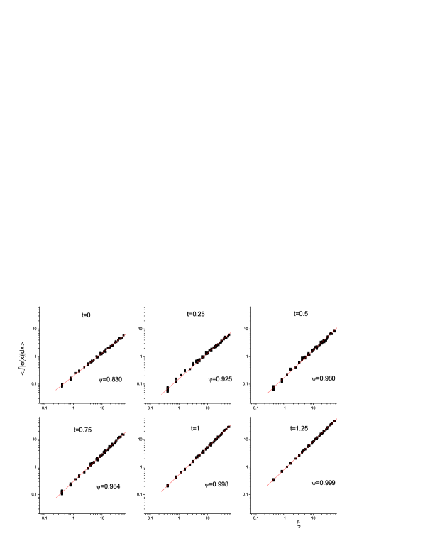
Figure 5: $\langle\int^{x_{0}+\xi}_{x_{0}}|\sigma(x)|dx\rangle$ versus $\xi$, for successive times $t=0$, $t=0.25$, $t=0.5$, $t=0.75$, $t=1$, $t=1.25$, for $A=1$ and $\lambda=1$ in dimensionless units. We observe that although the initial fractal mass dimension changes, the power law property remains valid as time evolves.

However, a more detailed analysis for greater time intervals reveals a remarkable phenomenon. In the solid line plots of fig. 6 we show the evolution of $\psi$ (each $\psi$ value coming from a linear fit).

Figure 6: Time evolution of the slope $\psi$ (solid line) and its time average $\langle\psi\rangle_{t}$ (dotted line) for varied $A$ and $\lambda$ in dimensionless units.

It can be clearly observed that the characteristic exponent $\psi(t)$ after reaching the value 1, fluctuates and for particular times becomes almost equal to $\psi(0)=5/6$. Thus, the initial fractal measure is restored repeatedly within the considered ensemble. A simultaneous study of this graph and fig. 3 is illuminating, since we observe that the reappearance of the fractal mass dimension, describing the initial measure, occurs when the mean field value becomes almost zero.

If we interpret the $\sigma$-field as a system of coupled anharmonic oscillators with initial field values around zero and zero kinetic energy, we expect an almost simultaneous pass from their turning points, due to synchronization. The energy transfer between the different oscillators takes place through the spatial derivative, as can be seen in equation (3). Therefore, if it is small compared to the other terms (which is the case in general), the oscillators do not mix significantly, and due to their initial zero kinetic energy they roll to their common minimum, they oscillate around it and then return to their starting position almost in phase and with kinetic energy close to the initial one, i.e close to zero. So, every time the kinetic energy and the mean field value become zero, the system reaches to a state similar to the initial one, leading to the restoration of the initial fractal measure. On the other hand, when the oscillators roll away from zero, the geometrical characteristics of the ensemble are changed by the dynamics, since they acquire large field values and large kinetic energy (compared to the initial ones).

In figs 6b,c,d we can clearly observe this behavior. Moreover, $\psi(t)$ in figs 6e and f is also easily interpreted since in these cases, following closely the evolution of the $\sigma$ mean value, it stabilizes after some reciprocations. Finally, the behavior of $\psi$ for $A=0$, $\lambda=0$ depicted in fig. 6a is also expected since in this case (3) reduces to the simple wave equation, $\sigma$ values stay always around zero, i.e around their initial values, and $\psi$ oscillates around a value between $5/6$ and $1$, namely the signs of the initial fractal geometry are always visible. The dotted line plots of fig. 6 depict the time average of $\psi$ defined by $\langle\psi\rangle_{t}=\frac{1}{t}\int_{0}^{t}\psi(t^{\prime})dt^{\prime}$. As it can be observed, the influence of the initial fractal mass dimension is still visible in this time integrated measure.

Lastly, in order to have a clearer apprehension of the aforementioned phenomenon, we perform some tests. In fig. 7a and 7b we present the evolution of the system with random initial conditions, prepared choosing the $\sigma$ value at each site from a uniform distribution, for $A=1$ and $\lambda=1$. The mean field value oscillates around the minimum as before, and the slope $\psi$ which initially is obviously one, corresponding to a non-fractal system, remains equal to 1 as expected, independently of the field motion. Following the arguments referred above, one could say that every time $\langle\sigma\rangle$ returns to zero the system enters in a state similar to the initial one, and $\psi(t)$ remains always 1 since the initial state is characterized by $\psi(0)=1$. In figs 7c and 7d we evolve our system using initial conditions corresponding to a fractal measure with mass dimension $\psi(0)=5/6$, but with random non-zero (actually quite large) kinetic energy, for $A=1$, $\lambda=1$. In this case the finite value of the initial kinetic energy (different for every oscillator) forbids the return of the system to a state close to the initial one, each time the mean value of the field passes through zero, suppressing the approach to the initial fractal state. (Note that due to the large initial kinetic energy the system oscillates around both minima).

Additionally, in figs 7e and 7f we perform the following scenario: We evolve the initial ensemble, possessing fractal mass dimension $\psi(0)=5/6$, for $A=1$, $\lambda=1$, introducing by hand a three orders of magnitude larger coefficient to the spatial derivative term in the equation of motion. As expected, the enhanced diffusion in this case induces very strong mixing of the oscillators, and as a consequence the system never reacquires the initial fractal characteristics .

Figure 7: Mean field, $\psi(t)$ (solid line) and $\langle\psi\rangle_{t}$ (dotted line) evolution for various scenarios. a) and b) correspond to random non-fractal initial conditions for $A=1$ and $\lambda=1$, c) and d) correspond to initial conditions with fractal mass dimension $\psi(0)=5/6$ and non-zero, randomly chosen, initial kinetic energy, for $A=1$ and $\lambda=1$, and e) and f) correspond to initial conditions with fractal mass dimension $\psi(0)=5/6$, zero kinetic energy, but three orders of magnitude larger spatial derivative term, for $A=1$ and $\lambda=1$.

IV Evolution of a scalar field configuration with deterministic fractal measure

In order to acquire a better comprehension of the mechanism of the aforementioned phenomenon, we investigate the evolution of one Cantor-like scalar field configuration. This set up, although not related to critical phenomena, is enlightening since in this case a direct geometrical interpretation at the level of one configuration is possible, instead of investigating the statistical fractal properties of an ensemble.

Firstly, we construct a finite approximation to the 1D Cantor dust of $2^{11}$ sites, with Hausdorf fractal dimension $D_{f}=5/6$ Mandel83 ; lala . In order to transform this fractal set into a field configuration defining a fractal measure on an equidistant lattice we find the minimum two-point distance of the set and using it as the lattice spacing we determine the size of the lattice by dividing the maximum two point distance in the set by the minimum one. In the sites of this new equidistant lattice that are closer to the locations of the points of the initial Cantor set, we give the field value 1, while in all the others we give the field value 0. Thus, we turn out with a field configuration in an equidistant lattice, which by construction has the property $\langle\int^{x_{0,i}+\zeta}_{x_{0,i}}|\sigma(x)|dx\rangle\propto\zeta^{D_{f}}$ in a good precision, where the reference sites $x_{0,i}$ ($i=1,...,2^{11}$) are obviously only those with field values 1. The averaging now is taken only on the different $x_{0,i}$ since we have only one configuration. The produced $\sigma$-field configuration is depicted in fig. 8 where the fractal property is clear. Note that starting from the initial $2^{11}$ Cantor lattice, we transited in a much larger ($\approx 2\times 10^{4}$ sites) equidistant one.

Figure 8: The $\sigma$-field derived by a Cantor-like fractal, on the equidistant lattice.

Now, we evolve this $\sigma$-configuration according to equation of motion (3) taking zero initial kinetic energy, and we focus on the evolution of $\langle\int^{x_{0,i}+\zeta}_{x_{0,i}}|\sigma(x)|dx\rangle$, which initially has the characteristic fractal mass dimension $\psi(0)=D_{f}=5/6$ as can be seen in the upper graph of fig. 10.

Figure 9: Mean field, standard deviation and $\psi$ (solid line) and $\langle\psi\rangle_{t}$ (dotted line) evolution for the deterministic fractal case, for $A=1$ and $\lambda=1$, in dimensionless units.

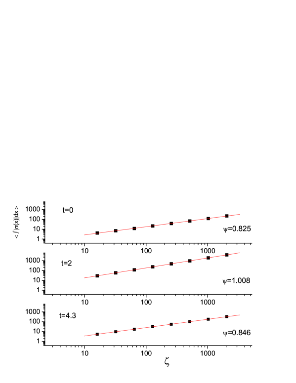
Figure 10: $\langle\int^{x_{0,i}+\zeta}_{x_{0,i}}|\sigma(x)|dx\rangle$ versus $\zeta$, for successive times $t=0$ (initial moment), $t=2$ (corresponding to the first complete destruction of the initial power law), and $t=4.3$ (corresponding to the first restoration of the initial fractal measure), for $A=1$ and $\lambda=1$, in dimensionless units.

In fig. 9 we demonstrate the evolution of the mean value of the field, its standard deviation, and the slope $\psi$, for potential parameters $A=1$ and $\lambda=1$. We observe the same behavior with the case of the previous section, that is the change of the initial fractal mass dimension, and its return to this value each time $\langle\sigma\rangle$ approaches zero. The explanation is the same as before without any significant new ideas. The only difference is that in the present case only a small subset of the entire lattice is initially described by a fractal measure with mass dimension $5/6$. The remaining lattice sites are occupied by zero field values, which initially have zero contribution to $\langle\int^{x_{0,i}+\zeta}_{x_{0,i}}|\sigma(x)|dx\rangle$. However, as the system evolves, these initially zero oscillators roll towards the potential minimum, producing a non-fractal background, i.e a linear contribution to $\langle\int^{x_{0,i}+\zeta}_{x_{0,i}}|\sigma(x)|dx\rangle$, and thus supplanting and suppressing the total power law behavior. On the other hand, when the mean field value returns to zero, the system reaches a state similar to the initial one, (zero mean field value and zero kinetic energy), the initially zero oscillators approach again the value $\sigma=0$ almost in phase and reproduce a configuration with fractal mass dimension $D_{f}\approx 5/6$. In fig. 10 we depict $\langle\int^{x_{0,i}+\zeta}_{x_{0,i}}|\sigma(x)|dx\rangle$ versus $\zeta$ for three times. The first corresponds to the initial moment, the second to the first complete destruction of the fractal geometry, and the third to the first approximate re-establishment of the initial fractal measure.

V Two coupled fields

It is interesting to extend the single field model of section II in the case of two coupled fields, one of them having a fractal profile and the other a conventional one. In this case the Lagrangian density (1) is extended to

$$\mathcal{L}=\frac{1}{2}(\partial_{\mu}\sigma\partial^{\mu}\sigma+\partial_{\mu}\pi\partial^{\mu}\pi)-V(\sigma,\pi),$$ (9)

with the potential

$$V(\sigma,\pi)=\frac{\lambda}{4}(\sigma^{2}+\pi^{2}-1)^{2}-A\sigma,$$ (10)

avoiding to introduce additional parameters. The fields are defined in $1+1$ dimensions. The equations of motion derived from (9) are

$$\ddot{\sigma}-\sigma^{\prime\prime}+\lambda\sigma^{3}+\lambda(\pi^{2}-1)\sigma-A=0$$

$$\ddot{\pi}-\pi^{\prime\prime}+\lambda\pi^{3}+\lambda(\sigma^{2}-1)\pi=0.$$ (11)

We are interested in studying the evolution of our system determined by the above equations, taking for the $\sigma$-field initial conditions possessing fractal behavior as described in section II, and for the $\pi$-field conventional initial conditions, corresponding to an ideal gas at temperature $T_{0}$. In the next subsection we describe the generation of the ensemble of 1-d $\pi$-configurations on the lattice, using the algorithm introduced in Cooper .

V.1 Generation of thermal $\pi$-configurations

The unperturbed Hamiltonian for the classical scalar field theory in 1-d is

$$H=\frac{1}{2}\int^{+\infty}_{-\infty}dx[(\partial_{t}\pi(x,t))^{2}+(\partial_{x}\pi(x,t))^{2}+m_{\pi}^{2}\pi(x,t)^{2}].$$ (12)

The free particle solutions for $t=0$ are

$$\pi(x,0)=\int^{+\infty}_{-\infty}\frac{dk}{2\pi}\pi_{k0}\,e^{ikx}=\int^{+\infty}_{-\infty}\frac{dk}{2\pi}\frac{(a_{k}+a_{-k}^{\ast})}{\sqrt{2\omega_{k}}}e^{ikx}$$

$$\dot{\pi}(x,0)=\int^{+\infty}_{-\infty}\frac{dk}{2\pi}\xi_{k0}\,e^{ikx}=\int^{+\infty}_{-\infty}\frac{dk}{2\pi}\sqrt{\frac{\omega_{k}}{2}}i(a_{-k}^{\ast}-a_{k})e^{ikx}.$$ (13)

where $\omega_{k}=\sqrt{k^{2}+m_{\pi}^{2}}$.

Now, choosing an initial classical density distribution Cooper

$$\rho[\pi,\dot{\pi}]=Z^{-1}(\beta_{0})\,\exp{\left\{-\beta_{0}\,H[\pi,\dot{\pi}]\right\}},$$ (14)

and substitute the Hamiltonian (12) with the free particle solutions (13), we finally acquire

$$\rho[x_{k},y_{k}]=Z^{-1}(\beta_{0})\,\exp{\left\{-\beta_{0}\,\int^{+\infty}_{-\infty}\frac{dk}{2\pi}\omega_{k}(x_{k}^{2}+y_{k}^{2})\right\}},$$ (15)

with $\beta_{0}=1/T_{0}$, and where: $a_{k}=x_{k}+iy_{k}$ with $x_{k},y_{k}$ real. In order to produce a thermal ensemble (at temperature $T_{0}$) of configurations for $\pi(x,0)$ and $\dot{\pi}(x,0)$, we select $x_{k}$ and $y_{k}$ from the gaussian distribution (15), assemble $a_{k}$ and then substitute in (13).

Figure 11: The $\pi$-field on the lattice averaged over the ensemble of configurations.

The corresponding $\langle\pi(x)\rangle$ profile is shown in fig. 11. All the characteristics of the $\pi$-ensemble such as the correlation function $\langle\pi(x)\pi(x+\delta x)\rangle-\langle\pi(x)\rangle\langle\pi(x+\delta x)\rangle$, which turns out to be a $\delta$-function, are consistent with the assumption of an ideal thermal gas.

V.2 Numerical Results. Two coupled fields

We solve equations of motion (11) in 1-D 2000-site lattice following the discretization scheme (4), using for initial conditions an ensemble of $10^{4}$ $\sigma$ and $\pi$ configurations satisfying the aforementioned requirements, that is fractal $\sigma$ and conventional $\pi$ (corresponding to dimensionless temperature $T_{0}=1$) configurations. As in the single field case we focus on the evolution of the $\langle\int^{x_{0}+\xi}_{x_{0}}|\sigma(x)|dx\rangle$, which defines a fractal measure, initially having the characteristic mass dimension $5/6$, generated by the $\sigma$-field.

Figure 12: Mean field and standard deviation evolution in the two-field case for $A=1$, $\lambda=1$, in dimensionless units. Mind the different vertical axis scale in plot c).

In figs 12a,b we demonstrate the evolution of the mean $\sigma$-field and its standard deviation, and in figures 12c,d the corresponding quantities for the $\pi$-field, for $A=1$ and $\lambda=1$. The absence of a term linear in $\pi$-field in the potential (10), leads to slight oscillations, due to the small initial total energy of the $\pi$-field, of the mean value $\langle\pi\rangle$ around zero. The anharmonic character of these oscillations relies on the non-linear form of the equation of motion (11), and is enhanced relatively to the $\sigma$ case due to the large variation of the coupling term $\lambda(\sigma^{2}-1)\pi$. Note however that although the mean field value $\langle\pi\rangle$ remains small, this is not the case for its fluctuations which can become quite large. On the other hand, as one can see in figures 12a,b, the corresponding $\sigma$ quantities do not differ significantly from the single field case since $\pi$-field remains small.

Figure 13: Time evolution of the slope $\psi$ (solid line) and its time average $\langle\psi\rangle_{t}$ (dotted line) in the two-field case, for $A=1$ and $\lambda=1$, in dimensionless units.

In fig. 13 we depict the slope $\psi(t)$ for the aforementioned evolution scenario of the $\sigma$-field interacting with the $\pi$-field. In general we observe the same phenomenon as in the single field case, that is $\psi(t)$ becomes approximately equal to its initial value every time $\langle\sigma\rangle$ approaches zero. However, the stronger non-linearity forbids $\langle\sigma\rangle$ to become exactly zero but rather to obtain a small finite value, which in turn has as a consequence that $\psi(t)$ does not approach so closely the initial value as in the single field case. This is illustrated in figs. 13 and  12a, at $t\sim 4$ and $t\sim 9$, which correspond to the times when $\langle\sigma\rangle(t)$ has a local minimum. In the case of the first minimum ($t\sim 4$), $\langle\sigma\rangle$ returns closer to zero and therefore $\psi(t)$ becomes almost $5/6$, compared to the case of the second minimum at $t\sim 9$, when $\langle\sigma\rangle$ reaches a greater value ($\sim 0.5$) and correspondingly $\psi(t)$ deviates stronger from its initial value. However, in both cases the system maintains a memory of its initial fractal characteristics.

We have evolved the system with various $\pi$-field initial conditions (random, constant etc) in order to check the generality of the results described above. It turns out that for the two-field case the re-establishment of the initial fractal geometry does not depend on the specific $\pi$-field initial conditions, unless they are fine tuned so that $\langle\sigma\rangle$ is driven to large values without occasionally returning close to the region $\langle\sigma\rangle\approx 0$.

VI Discussion and Conclusions

In this work we investigate the evolution of the fractal characteristics of a single or two coupled scalar fields system, within the framework of the general $\sigma$-model. After a relatively rapid deformation of the initial fractal geometry, we observe that it is being re-established almost periodically each time the mean value of the $\sigma$-field returns to zero. This effect is obtained using both random, as well as deterministic (Cantor-like) fractal set up. The key point for the occurrence of this behavior is the condition of initial equilibrium. As the system practically consists of coupled anharmonic oscillators, this condition is expressed through the zero initial kinetic energy for each oscillator, leading to a synchronous evolution of the entire system. Additionally, the fractal measure characterizing the initial state is based on the fact that the corresponding field configurations represent fluctuations (with a specific pattern) around zero. Thus, each time the oscillators pass through their turning points, associated to zero mean field value, in phase, the initial fractal geometry is being re-established. The above evolution, at least qualitatively, is quite general and robust for a very wide parametric space.

The scenario analyzed in this paper could be extended to 3 dimensions and serve as a model in order to describe the evolution of the order parameter fluctuations in a critical system. In particular it could be used to explore the non-conventional correlations which are expected to occur during the formation of an isoscalar condensate in a heavy ion collision experiment. In this case one has to adapt the $\sigma$-model Lagrangian in order to describe correctly the characteristics of the order parameter associated with the 2nd order critical end point of the chiral QCD phase transition RW . At the phenomenological level these correlations are expressed through the fractal mass dimension of the $\sigma$-field configurations, determining the statistical properties of the condensate. The dynamics of the system is similar to the two-field case investigated above, provided that the critical system is initially at equilibrium. One can study the evolution of the initial fractal characteristics of the $\sigma$-field and the possibility to leave signals at the detectors, supplying an indication of the phase transition. The discussion of the present work supports this eventuality since the time average (in order to simulate the experimental conditions) of the periodical deformation and re-establishment of the initial fractal geometry, will leave a signature. The specific application of the present work in the case of QCD phase transition has been performed in Futurework .

Acknowledgements:

We thank V. Constantoudis and N. Tetradis for useful discussions. One of us (E.N.S) wishes to thank the Greek State Scholarship’s Foundation (IKY) for financial support. The authors acknowledge partial financial support through the research programs “Pythagoras” of the EPEAEK II (European Union and the Greek Ministry of Education) and “Kapodistrias” of the University of Athens.

References

- (1) M. Toda, Theory of nonlinear lattices, Springer Verlag (1989).
- (2) E. Fermi, J. Pasta, S. Ulam, Los Alamos Rpt. LA-1940, 20 (1955); also in ”Collected Works of E. Fermi”, University of Chicago Press, Vol II (1965).
- (3) J. Ford, Phys. Rep. 213, 271 (1992).
- (4) G. Parisi, Europhys. Lett, 40 (4), 357 (1997);
- (5) GF. Bonini, C. Wetterich, Phys. Rev. D 60, 105026 (1999)[arXiv: hep-ph/9907533]; GF. Bonini, C. Wetterich, Nucl.Phys. B 587, 1-3, 403 (2000) [arXiv:hep-ph/0003262]; S. Juchem, W. Cassing, C. Greiner, Phys. Rev. D 69, 025006 (2004)[arXiv:hep-ph/0307353].
- (6) B. B. Mandelbrot, The Fractal Geometry of Nature, W. H. Freeman and Company, New York (1983).
- (7) T. Vicsek, Fractal Growth Phenomena, World Scientific, Singapore (1999).
- (8) K. Falconer, Fractal Geometry: Mathematical Foundations and Applications, John Wiley & Sons, West Sussex (2003).
- (9) N. G. Antoniou et al, Phys. Rev. Lett. 81, 4289 (1998) [arXiv:hep-ph/9810383]; N. G. Antoniou, Y. F. Contoyiannis, F. K. Diakonos, Phys. Rev. E 62, 3125 (2000) [arXiv:hep-ph/0008047].
- (10) M. M. Tsypin, Phys. Rev. Lett. 73, 2015 (1994).
- (11) N. G. Antoniou, F. K. Diakonos, E. N. Saridakis and G. A. Tsolias, Physica A 376, 308 (2007) [arXiv:physics/0607038].
- (12) N. Metropolis et al, J. Chem. Phys. 21, 1087 (1953).
- (13) N. G. Antoniou, F. K. Diakonos, E. N. Saridakis and G. A. Tsolias, Phys. Rev. E 75, 041111 (2007) [arXiv:physics/0610111].
- (14) K. B. Blagoev, F. Cooper, J. F. Dawson and B. Mihaila, Phys. Rev. D 64, 125003 (2001).
- (15) K. Rajagopal and F. Wilczek, Nucl.Phys. 399, 395 (1993) [arXiv:hep-ph/9210253].
- (16) N. G. Antoniou, F. K. Diakonos, E. N. Saridakis, Nucl. Phys. A 784, 536 (2007) [arXiv:hep-ph/0610382]; N. G. Antoniou, F. K. Diakonos, E. N. Saridakis, Phys. Rev. C 78, 024908 (2008) [arXiv:0709.0339[hep-ph]].