How a Long Bubble Shrinks: a Numerical Method for an Unforced Hele-Shaw Flow

Abstract

We develop a numerical method for solving a free boundary problem which describes shape relaxation, by surface tension, of a long and thin bubble of an inviscid fluid trapped inside a viscous fluid in a Hele-Shaw cell. The method of solution of the exterior Dirichlet problem employs a classical boundary integral formulation. Our version of the numerical method is especially advantageous for following the dynamics of a very long and thin bubble, for which an asymptotic scaling theory has been recently developed. Because of the very large aspect ratio of the bubble, a direct implementation of the boundary integral algorithm would be impractical. We modify the algorithm by introducing a new approximation of the integrals which appear in the Fredholm integral equation and in the integral expression for the normal derivative of the pressure at the bubble interface. The new approximation allows one to considerably reduce the number of nodes at the almost flat part of the bubble interface, while keeping a good accuracy. An additional benefit from the new approximation is in that it eliminates numerical divergence of the integral for the tangential derivative of the harmonic conjugate. The interface’s position is advanced in time by using explicit node tracking, whereas the larger node spacing enables one to use larger time steps. The algorithm is tested on two model problems, for which approximate analytical solutions are available.

1 Introduction

Let a bubble of low-viscosity fluid (say, air) get trapped inside a high-viscosity fluid (say, oil) in a quasi-two-dimensional Hele-Shaw cell: two parallel plates with a narrow gap between them. What will happen to the shape of the bubble, if the (horizontal) plates of the Hele-Shaw cell are perfectly smooth, and the two fluids are immiscible? The answer depends on the initial bubble shape. A perfectly circular bubble (or an infinite straight strip) will not change, while a bubble of any other shape will undergo surface-tension-driven relaxation until it either becomes a perfect circle, or breaks into two or more bubbles, which then become perfect circles. The bubble shape relaxation process is non-local, as it is mediated by a flow in the external viscous fluid. The two-dimensional surface-tension-driven flow can be called an unforced Hele-Shaw (UHS) flow. This is in contrast to forced Hele-Shaw flows that have been in the focus of hydrodynamics and nonlinear and computational physics for the last two decades [1, 2, 3, 4, 5]. In rescaled variables, the UHS flow is described by the solution of the following free boundary problem, see e.g. Refs. [6, 7]:

$$\nabla^{2}p(q)=0\qquad\mbox{for}\qquad q\in E,$$ (1)

$$p(q)=\mathcal{K}\qquad\mbox{for}\qquad q\in\gamma,$$ (2)

$$v_{n}(q)=-\nabla_{n}p(q)\qquad\mbox{for}\qquad q\in\gamma,$$ (3)

where $E$ is an unbounded region of the plane, external to the bubble interface $\gamma$, $v_{n}$ is the normal velocity of the interface, the index n denotes the component of vectors normal to the interface, and $K$ is the local curvature of the interface. The pressure $p$ is bounded at infinity. The free boundary problem (1)-(3) splits into two sub-problems:

1. Solving the exterior Dirichlet problem (1) and (2) and calculating $v_{n}(q)$ from Eq. (3).

2. Advancing the interface $\gamma$ in time with the known $v_{n}(q)$.

The free boundary problem (1)-(3) represents an important example of area-preserving curve-shortening motion [8], but it is not integrable. Moreover, the only analytical solution to this problem, available until recently, was the approximate solution following from a linear stability analysis of a slightly deformed circular or flat interface [9]. Recently an asymptotic scaling theory has been developed for a non-trivial case when the inviscid fluid occupies, at $t=0$, a half-infinite (or, physically, very long) strip [7]. It turned out that this somewhat unusual initial condition provides a useful characterization of the UHS flow, as the evolving strip, which develops a dumbbell shape, exhibits approximate self-similarity with non-trivial dynamic exponents [7]. Predictions of the scaling analysis have been verified numerically in Ref. [7] by using a boundary integral algorithm, tailored to the very large aspect ratio of the bubble. The present paper describes this algorithm in detail.

A multitude of numerical methods have been suggested in the recent years for simulating different variants of Hele-Shaw flows. Boundary integral methods, which deal directly with the interface between the two fluids, are advantageous compared to methods of finite elements and finite differences. Methods based on conformal mapping techniques have long been used in this class of problems (see, e.g. Refs. [2, 11, 12]). However, they apply most naturally to the case of zero surface tension and are less convenient when surface tension is non-zero [10]. Still another numerical strategy is phase field methods. Folch et al. [13, 14] developed a phase field method for an arbitrary ratio of the viscosities of the two fluids. Unfortunately, their method becomes inefficient when the viscosity contrast is too high [14]. To remind the reader, the viscosity contrast is infinite in the case under consideration in the present work. Glasner [15] developed a phase field method for a description of a bubble of a high-viscosity fluid trapped in a low-viscosity fluid. We are unaware of any phase-field approach which would deal with the opposite case, which is under investigation in the present work: a low-viscosity bubble in a high-viscosity fluid.

The present work suggests a numerical algorithm for solving the free boundary problem (1)-(3) in the special case of a very long bubble. It is well-known (but still remarkable) that the exterior Dirichlet problem (1) and (2) can be formulated in terms of a Fredholm integral equation of the second kind for an effective density of the dipole moment [16]. A naïve formulation, however, would lead to non-existence of solution by the Fredholm alternative [17]. To overcome this difficulty, Greenbaum et al. [17] implemented in their algorithm a modification of the Fredholm equation due to Mikhlin [18]. The modified Fredholm equation has a unique solution for any smooth $\gamma$ and integrable $\mathcal{K}$ [18]. Greenbaum et al. developed an efficient numerical algorithm (which is also valid for multiple bubbles) by discretization. However, the geometry of a very long and thin bubble, that we are mostly interested in, defines widely different length scales in the problem. Rapid variations of the dipole moment density at the highly curved ends of the bubble naturally necessitate a small spacing between the interface nodes. It is less natural, however, that, in a straightforward approach, one must keep the node spacing much smaller than the bubble thickness over the whole bubble interface. Indeed, as we show below, the typical length scale of the variation of the kernel of the integral equation is comparable to the bubble thickness which, during the most interesting part of the long bubble dynamics, remains almost unchanged. Apart from being computationally inefficient, the straightforward approach would cause a problem for explicit tracking of nodes, as the stability criterion, intrinsic in the explicit method, demands a time step less then a constant $\mathcal{O}(1)$ multiplied by the node spacing cubed [19]. In this work we turned this obstacle into advantage, by employing the fact that the length scale of variation of the solution, over the most of the bubble interface, is much greater than the bubble thickness. We constructed a new approximation of the integral entering the Fredholm equation, by representing the sought dipole moment density as a piecewise constant function, and the bubble interface shape function as a piecewise linear function. As a result, the integral is approximated by a sum, each term of which is equal to a local value of the dipole moment density multiplied by an integral of the kernel between two neighboring nodes. Fortunately, the latter integral can be calculated analytically. The new approximation allowed us to considerably increase the node spacing over the most of the bubble interface, while keeping a good accuracy.

Having found an approximated solution $p$ in the form of a double layer potential, one needs to compute the normal derivative of the solution $\nabla_{n}p(q\in\gamma)$. In a straightforward realization of the boundary integral formulation this would result in a hypersingular integral, see Ref. [17]. To overcome this difficulty, one resorts to theory of analytic functions and computes the harmonic conjugate $V(q)$. By virtue of the Cauchy-Riemann equations, the tangential derivative of $V(q)$ is equal to the desired normal derivative of $p$. The harmonic conjugate $V(q)$ has the form of a principal value integral, over the interface, of the dipole moment density multiplied by a kernel, which is a function of coordinates of two points, $q$ and $g$, belonging to the interface. This kernel diverges when the integration variable $g$ coincides with $q$. Here we again employ the large scale difference at the flat part of the bubble and use the same approximation as in the Fredholm equation. As an additional benefit, the numerical divergence of the integrand of the harmonic conjugate $V$ is avoided. As a result, we do not need to use even nodes to compute $V$ at odd nodes and vice-versa, as suggested in Ref. [17].

Here is a layout of the rest of the paper. Section 2 deals with the numerical solution of the exterior Dirichlet problem, and with the computation of the normal derivative of the solution at the interface. We briefly review the boundary integral method for an exterior Dirichlet problem and motivate the need for its modification for very long bubbles. Then we formulate our discrete approximation. In Section 3 we briefly describe a simple explicit integration which we used to track the bubble interface. Section 4 presents the results of code testing, while Section 5 presents the Conclusions.

2 Exterior Dirichlet Problem

2.1 Boundary integral formulation

Following Mikhlin [18], we seek the solution $p(q)$ of the problem(1) and (2) for a simply connected bubble in a double layer potential representation:

$$p(q)=\frac{1}{2\pi}\oint_{\gamma}\left[1+K(q,g)\right]\mu(g)\,dg\;\;\;\mbox{for}\;\;q\in E,$$ (4)

where $\mu(g)$ is an unknown dipole density at the point $g$ of the interface, and $dg$ is the element of arclength including the point $g$. The kernel $K(q,g)=\cos\alpha/|\vec{r}(q,g)|$ follows from classical potential theory [16]. Here $\alpha$ is the angle between the outward normal to the interface at the point $g$ and the vector $\vec{r}(q,g)$, see Fig. 1.

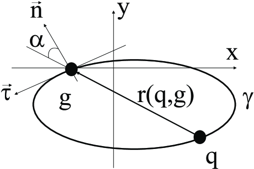
Figure 1: Geometry of the kernel $K(q,g)$. $\vec{\tau}$ and $\vec{n}$ are the tangential and outward normal directions, respectively.

The boundary condition (2) can be rewritten as an integral equation for $\mu(q)$, see, e.g., [16]:

$$-\mu(q)+\frac{1}{\pi}\oint_{\gamma}\left[1+K(q,g)\right]\mu(g)\,dg=2\mathcal{K}(q)\,.$$ (5)

That is, to compute $p(q)$ in Eq. (4), one needs to solve the integral equation (5). Mikhlin [18] showed that Eq. (5) has a unique solution for any smooth $\gamma$ and integrable $\mathcal{K}$, while $p(q)$ from Eq. (4) is a harmonic function in the exterior, satisfying the boundary condition Eq. (2). This representation was employed by Greenbaum et al. [17] for numerical analysis.

For the purposes of the free boundary problem (1)-(3) one only needs the value of $\nabla_{n}p(q)$, $p\in\gamma$. A straightforward calculation of $\nabla_{n}$ from the double layer potential would yield a hypersingular integral, see below. One circumvents this difficulty by resorting to theory of analytic functions, see Ref. [17] and references therein. Suppose $\mu(q)$ is known and introduce the quantity

$$\tilde{p}(q)=\frac{1}{2\pi}\oint_{\gamma}\mu(g)K(q,g)\,dg\,,$$

which differs from $p(q)$ only by a constant, as $\oint_{\gamma}\mu(g)\,dg=\mbox{const}.$ Obviously, $\nabla_{n}\tilde{p}=\nabla_{n}p$. It is known [17] that $\tilde{p}(q)$ is the real part of the Cauchy integral

$$\frac{1}{2\pi i}\oint_{\gamma}\frac{\mu(\zeta)}{\zeta-z}d\zeta=\tilde{p}(z)+iV(z),$$

where we have identified the points $q$ and $g$ on the plane with respective complex numbers $z$ and $\zeta$. Then $\tilde{p}$ and its harmonic conjugate $V$ satisfy the Cauchy-Riemann equations, so that

$$\tilde{p}_{n}=V_{\tau}\,,$$ (6)

where the indices $n$ and $\tau$ stand for the normal and tangential derivatives, respectively. The kernel $K(q,g)$ can be written as follows:

$$K(q,g)\,dg=\frac{-(y_{g}-y_{q})\,dx_{g}+(x_{g}-x_{q})\,dy_{g}}{r^{2}(q,g)}\,,$$

where $x$ and $y$ are the Cartesian coordinates of the respective points. After a simple algebra we obtain

$$V(q)=-\frac{1}{2\pi}\oint_{\gamma}\frac{\mu(x_{g},y_{g})(x_{g}-x_{q})}{r^{2}(q,g)}\,dx_{g}+\frac{\mu(x_{g},y_{g})(y_{g}-y_{q})}{r^{2}(q,g)}\,dy_{g}\,.$$ (7)

2.2 Discrete approximation

Let us parameterize the closed interface $\gamma$ of the bubble: $x=x(\sigma)$, $y=y(\sigma)$, $0\leq\sigma\leq M$, $x(0)=x(M)$, $y(0)=y(M)$, where $x$ and $y$ are the Cartesian coordinates of a point belonging to the interface. In the parametric form Eq. (5) becomes

$$-\mu(\sigma)+\frac{1}{\pi}\int_{0}^{M}\mu(\xi)\left[1+\kappa(\sigma,\xi)\right]\sqrt{\dot{x}^{2}+\dot{y}^{2}}\,d\xi=2\mathcal{K}(\sigma)\,,$$ (8)

where

$$\kappa(\sigma,\xi)=\frac{\dot{y}[x(\xi)-x(\sigma)]-\dot{x}[y(\xi)-y(\sigma)]}{\{[x(\sigma)-x(\xi)]^{2}+[y(\sigma)-y(\xi)]^{2}\}\sqrt{\dot{x}^{2}+\dot{y}^{2}}}\,,$$ (9)

while $\dot{x}=dx/d\xi$ and $\dot{y}=dy/d\xi$. The harmonic conjugate takes the form

$$V(\sigma)=-\frac{1}{2\pi}\int_{0}^{M}\mu(\xi)\frac{\dot{x}[(x(\xi)-x(\sigma)]+\dot{y}[(y(\xi)-y(\sigma)]}{[(x(\xi)-x(\sigma)]^{2}+[(y(\xi)-y(\sigma)]^{2}}\,d\xi.$$ (10)

Note that the kernel $\kappa$ is continuous as $\xi\to\sigma$. On the contrary, the integrand in the last expression diverges as $\xi\to\sigma$, and the integral exists only as a principal value.

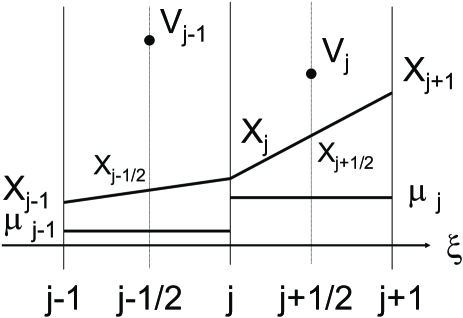
Figure 2: The discrete approximation scheme. Here $\xi_{j}=j.$

In the main case of our interest the bubble length is much greater than its thickness $\Delta$. In the almost flat parts of the interface $\dot{y}\approx 0$. Now, $y(\sigma)-y(\xi)\sim\Delta$ when the points $\sigma$ and $\xi$ belong to the different (upper and lower) parts of the interface, while $y(\sigma)-y(\xi)\approx 0$ when they belong to the same part of the interface. Then, using the relation $\dot{x}=dx/d\xi$, we can estimate the kernel $\kappa$ as

$$\kappa(\sigma,\xi)\,d\xi\approx\frac{-\Delta}{[x(\sigma)-x(\xi)]^{2}+\Delta^{2}}\,dx\,,$$ (11)

when $\sigma$ and $\xi$ belongs to the different parts of the interface, while $\kappa\approx 0$ when they belong to the same part. Equation (11) shows that the typical scale of variation of the kernel (9) over the almost flat part of the interface is of order of the bubble thickness $\Delta$. A similar estimate applies to the fraction entering the integrand of Eq. (10). A straightforward discretization would then require a node spacing much less than $\Delta$. Instead, we rewrite Eq. (8) as

$$-\mu(\sigma)+\frac{1}{\pi}\sum_{j=0}^{m-1}\int_{\xi_{j}}^{\xi_{j+1}}\mu(\xi)[1+\kappa(\sigma,\xi)]\sqrt{\dot{x}^{2}+\dot{y}^{2}}\,d\xi=2\mathcal{K}(\sigma)\,,$$ (12)

where $\xi_{0}=0$, $\xi_{m}=M$, and $\xi_{j+1}>\xi_{j}$, $j=0,1,2,\dots,m-1$. Introduce a piecewise linear approximation for $x(\xi)$ and $y(\xi)$ (see Fig. 2):

$$x(\xi)=k_{j}^{x}\xi+b_{j}^{x},\quad y(\xi)=k_{j}^{y}\xi+b_{j}^{y},$$ (13)

where $\xi_{j}\leq\xi\leq\xi_{j+1},\quad j=0,1,2,\dots,m-1,$ $k_{j}^{x}=(x_{j+1}-x_{j})/(\xi_{j+1}-\xi_{j})$, $b_{j}^{x}=(\xi_{j+1}x_{j}-\xi_{j}x_{j+1})/(\xi_{j+1}-\xi_{j})$, $k_{j}^{y}=(y_{j+1}-y_{j})/(\xi_{j+1}-\xi_{j})$, $b_{j}^{y}=(\xi_{j+1}y_{j}-\xi_{j}y_{j+1})/(\xi_{j+1}-\xi_{j})$, $x_{j}=x(\xi_{j})$, $y_{j}=y(\xi_{j}),$ and a piecewise constant approximation for $\mu$:

$$\mu(\xi)=\mu_{j}=\mbox{const},\qquad\xi_{j}\leq\xi\leq\xi_{j+1},$$ (14)

Note that $\dot{x}(\xi_{j}\leq\xi\leq\xi_{j+1})=k^{x}_{j},$ $\dot{y}(\xi_{j}\leq\xi\leq\xi_{j+1})=k^{y}_{j}$. The kernel (9) is therefore approximated as

$$\kappa(\sigma,\xi)=\frac{k^{y}_{j}[k^{x}_{j}\xi+b^{x}_{j}-x(\sigma)]-k^{x}_{j}[k^{y}_{j}\xi+b^{y}_{j}-y(\sigma)]}{\{[k^{x}_{j}\xi+b^{x}_{j}-x(\sigma)]^{2}+[k^{y}_{j}\xi+b^{y}_{j}-y(\sigma)]^{2}\}S_{j}}=\frac{Q_{j}(\sigma)/S_{j}}{S_{j}^{2}\xi^{2}+B_{j}(\sigma)\xi+C_{j}(\sigma)},$$

where

$$S_{j}=\sqrt{(k^{x}_{j})^{2}+(k^{y}_{j})^{2}},\quad Q_{j}(\sigma)=k^{y}_{j}[b^{x}_{j}-x(\sigma)]-k^{x}_{j}[b^{y}_{j}-y(\sigma)]\,,$$

$$B_{j}(\sigma)=2\{k^{x}_{j}[b^{x}_{j}-x(\sigma)]+k^{y}_{j}[b^{y}_{j}-y(\sigma)]\},\;\;\mbox{and}\;\;C_{j}(\sigma)=[b^{x}_{j}-x(\sigma)]^{2}+[b^{y}_{j}-y(\sigma)]^{2}\,.$$

The integrals in (12) can be calculated analytically:

$$\int_{\xi_{j}}^{\xi_{j+1}}\mu(\xi)[1+\kappa(\sigma,\xi)]\sqrt{\dot{x}^{2}+\dot{y}^{2}}\,d\xi=\mu_{j}\int_{\xi_{j}}^{\xi_{j+1}}\left[S_{j}+\frac{Q_{j}(\sigma)}{S_{j}^{2}\xi^{2}+B_{j}(\sigma)\xi+C_{j}(\sigma)}\right]\,d\xi=$$

$$=\mu_{j}\left\{S_{j}(\xi_{j+1}-\xi_{j})+\frac{1}{Q_{j}(\sigma)}\left[\arctan\frac{2S_{j}^{2}\xi_{j+1}+B_{j}(\sigma)}{2Q_{j}(\sigma)}-\arctan\frac{2S_{j}^{2}\xi_{j}+B_{j}(\sigma)}{2Q_{j}(\sigma)}\right]\right\}.$$

It is convenient to define $\xi_{j}=j$, then $\xi_{j+1}-\xi_{j}=1$. In our discretization scheme $x(\sigma)=x_{i+1/2}=k_{i}^{x}(i+1/2)+b_{i}^{x}$ and $y(\sigma)=y_{i+1/2}=k_{i}^{y}(i+1/2)+b_{i}^{y}$. Let us denote $Q_{j}(\sigma)=Q_{ij}$, $B_{j}(\sigma)=B_{ij}$, and $C_{j}(\sigma)=C_{ij}.$ The integrals in Eq. (12) are

$$\int_{\xi_{j}}^{\xi_{j+1}}\mu(\xi)[1+\kappa(\sigma,\xi)]\sqrt{\dot{x}^{2}+\dot{y}^{2}}\,d\xi=\pi\mu_{j}\textsc{A}_{ij},$$

where

$$\textsc{A}_{ij}=\frac{1}{\pi}\left\{S_{j}+\frac{1}{Q_{ij}}\arctan\frac{4S_{j}^{2}Q_{ij}}{4Q_{ij}+(2S_{j}^{2}j+B_{ij})[2S_{j}^{2}(1+j)+B_{ij}]}\right\}.$$

We have arrived at a set of linear algebraic equations with respect to $\mu_{j}$, which is our approximation of the integral equation (5):

$$\sum_{j=0}^{m-1}(\textsc{A}_{ij}-\delta_{ij})\mu_{j}=2\mathcal{K}_{i},\quad i=0,1,2,3,\dots,m-1\,.$$ (15)

We approximate the interface curvature $\mathcal{K}(\sigma)$ by finite differences:

$$\mathcal{K}(\sigma=i+1/2)=\mathcal{K}_{i}=\frac{\ddot{y}_{i+1/2}\dot{x}_{i+1/2}-\ddot{x}_{i+1/2}\dot{y}_{i+1/2}}{[(\dot{y}_{i+1/2})^{2}+(\dot{x}_{i+1/2})^{2}]^{3/2}},$$

where $\dot{x}_{i+1/2}=k_{i}^{x}$, $\dot{y}_{i+1/2}=k_{i}^{y}$, $\ddot{x}_{i+1/2}=x_{i+2}-x_{i+1}-x_{i}+x_{i-1}$, and $\ddot{y}_{i+1/2}=y_{i+2}-y_{i+1}-y_{i}+y_{i-1}$. Importantly, our approximation scheme yields the principal value of the integral (10) automatically. Furthermore, we can directly compute the coefficients $\textsc{A}_{ij}$, using the same expression for $i\neq j$ and $i=j$, where the kernel (9) has a removable discontinuity. The method suggested in [17] prescribes instead to use an analytic evaluation of the kernel at the point of removable discontinuity.

We solved the algebraic equations (15) by an iterative refinement method after a LU factorization of the matrix. As the maximum number of equations in the examples that we considered (see below) did not exceed $1100$, there was no need to use more sophisticated methods.

2.3 Grid

Most of our results were obtained with the version of the code which assumed a four-fold symmetry of the bubble. This allowed us to work with a one quarter of the interface and reduce the number of nodes by 4. In the beginning of the bubble relaxation, the solution varies rapidly in the region of the lobes, and very slowly in the flat region of the bubble. Therefore one should employ here a non-uniform grid. At later times, when the aspect ratio of the bubble becomes comparable to unity, the code switches to a uniform grid. For the non-uniform grid we used an exponential spacing. Here the node spacing grows exponentially from the lobe’s end to the middle of the flat part of the bubble. To generate the node distribution we use the following procedure. Let the quarter of the interface perimeter be $\Pi$, the specified number of nodes be $m$, and the specified smallest spacing in the lobe region be $h_{0}$.

If $\Pi>h_{0}(m-1)$, the exponential grid is used. Here we introduce the quantity $\eta$ which satisfies the condition

$$\Pi=h_{0}+\eta h_{0}+\eta^{2}h_{0}+\ldots+\eta^{m-2}h_{0}=\frac{h_{0}(1-\eta^{m-1})}{1-\eta}\,,$$ (16)

solve Eq. (16) numerically for $\eta$, use a discrete arclength parametrization: $\xi_{1}=0,\quad\xi_{2}=h_{0},\dots,\xi_{k}=\eta^{k-2}h_{0},\dots,\xi_{m}=\eta^{m-2}h_{0}$, and calculate the arrays $x=x(\xi_{i})$ and $y=y(\xi_{i})$, where $i=1,2,\dots,m$.

In the process of the interface evolution $\Pi$ decreases with time, so one can reduce the number of the grid nodes. Furthermore, as the nodes in our code move like lagrangian particles (see Section 3), the node spacing in the lobe region decreases with time even faster. If left unattended, this would cause instability of the node tracking (see Section 3), as the maximum allowed time step is proportional to the node spacing cubed [19]. Therefore, when the minimum node spacing decreases below $\xi_{2}=0.8h_{0}$, we redistribute the nodes: we look for the new value of $\eta$, corresponding to the updated value of $\Pi$, calculate the new array of $\xi$, and determine the new arrays $x$ and $y$ by linear interpolation.

When the perimeter goes down so that $\Pi\leq h_{0}(m-1)$, we switch to a uniform grid. Here we calculate a new $m$: $m=[\Pi/h_{0}]+1$, where $[a]$ is an integer number such that $0\leq a-[a]<1$, and fine tune $h_{0}$ so that $h_{0}=\Pi/(m-1)$.

Finally, the choice of $h_{0}$ is dictated by a compromise between the desired accuracy and the value of $m$ which determines the size of the matrix $A_{ij}$.

2.4 Calculation of the normal velocity

After the set of linear equations (15) is solved, and the quantities $\mu_{i}$ are found, we compute the harmonic conjugate $V$. The same approximation, applied to Eq. (10), yields:

$$V_{i}=-\frac{1}{2\pi}\sum_{j=0}^{m-1}\mu_{j}F_{ij}\,,$$

where

$$F_{ij}=\int_{j}^{j+1}\frac{k_{j}^{x}(k_{j}^{x}\xi+b_{j}^{x}-x_{i+1/2})+k_{j}^{y}(k_{j}^{y}\xi+b_{j}^{y}-y_{i+1/2})}{(k_{j}^{x}\xi+b_{j}^{x}-x_{i+1/2})^{2}+(k_{j}^{y}\xi+b_{j}^{y}-y_{i+1/2})^{2}}\,d\xi$$

$$=\frac{1}{2}\int_{j}^{j+1}\frac{2S_{j}^{2}\xi+B_{ij}}{S_{j}^{2}\xi^{2}+B_{ij}\xi+C_{ij}}\,d\xi=\frac{1}{2}\ln\frac{S_{j}^{2}(j+1)^{2}+B_{ij}(j+1)+C_{ij}}{S_{j}^{2}j^{2}+B_{ij}j+C_{ij}}\,,$$

where the quantities $S_{j}$, $B_{ij}$ and $C_{ij}$ were defined earlier. Again, the integral is calculated analytically. The resulting formula for $V_{i}$ is the following:

$$V_{i}=-\frac{1}{4\pi}\sum_{j=0}^{m-1}\mu_{j}\ln\frac{S_{j}^{2}(j+1)^{2}+B_{ij}(j+1)+C_{ij}}{S_{j}^{2}j^{2}+B_{ij}j+C_{ij}},$$ (17)

where $V_{i}=V(\sigma=i+1/2),$ $i=0,1,2,3,\dots,m-1$, see Fig. 2. Note that for $\xi=i+1/2$ the denominator of the integrand in $F_{ij}$ vanishes, and the integrand diverges. To overcome this problem, Ref. [17] suggested to divide the mesh into odd and even nodes and compute $V$ at the odd points by summing over the even nodes, and vice-versa. Our analytical integration yields the correct principal value of the integral, so there is no need to use the recipe of Ref. [17].

To compute the normal velocity of the interface we use the Cauchy-Riemann equation (6) and approximate the derivative of $V$ with respect to the arclength:

$$v_{n}(\sigma=i)=\frac{(V_{i+1}-V_{i})}{\tilde{s}_{i}}\,,$$

where

$$\tilde{s}_{i}=\frac{1}{2}\left[\sqrt{(x_{i+1}-x_{i})^{2}+(y_{i+1}-y_{i})^{2}}+\sqrt{(x_{i}-x_{i-1})^{2}+(y_{i}-y_{i-1})^{2}}\right].$$

3 Interface Tracking

To track the interface, we use an explicit first-order integration:

$$x_{i}(t+\Delta t)=x_{i}(t)+\Delta t\,v_{n}(\sigma=i,t)\cos n_{i},$$

$$y_{i}(t+\Delta t)=y_{i}(t)+\Delta t\,v_{n}(\sigma=i,t)\sin n_{i},$$

where

$$\cos n_{i}=\frac{\dot{y}_{i}}{\sqrt{\dot{x}^{2}_{i}+\dot{y}^{2}_{i}}}\,,\quad\sin n_{i}=-\frac{\dot{x}_{i}}{\sqrt{\dot{x}^{2}_{i}+\dot{y}^{2}_{i}}}\,,$$

$\dot{x}_{i}=(\dot{x}_{i+1/2}+\dot{x}_{i-1/2})/2=(k^{x}_{i}+k^{x}_{i-1})/2$, and $\dot{y}_{i}=(k^{y}_{i}+k^{y}_{i-1})/2$. We have assumed the counter-clockwise direction of the interface parametrization, see Fig. 1.

It is important to prescribe the time step $\Delta t$ properly. We employ an ad-hoc criterion which demands that the node displacement at each grid point be considerably less then the curvature radius $R_{i}$ at that point: $\min|(\Delta t\,v_{n}(i))/R_{i}|\leq\varepsilon,\quad 0\leq i\leq m-1.$ That is, we consider the curvature radius $R_{i}$ as a natural local length scale of the problem. A more convenient form of this criterion is

$$\Delta t=\varepsilon\min\{|R_{i}/v_{n}(i)|\}\,,$$ (18)

where $\varepsilon$ is an input parameter which has to be sufficiently small to satisfy the requirements of stability and desired accuracy. In the exact formulation (1)-(3) the bubble area must be constant in the process of relaxation. The area conservation can be conveniently used for accuracy control of the code.

4 Numerical Results

We present here some simulation results produced with our code for two different sets of initial conditions. One of them describes the decay of a small sinusoidal perturbation of a perfectly circular bubble of inviscid fluid. An approximate analytical solution to this problem is given by the linear stability analysis [9], and we used this solution to test the code.

The second initial condition describes a very long and thin strip of inviscid fluid. In the process of its shrinking the bubble develops a dumbbell shape, while the characteristic dimensions of the dumbbell exhibit asymptotic scaling laws found in Ref. [7].

4.1 Relaxation of a slightly perturbed circle

Let the initial shape of the interface be a circle with a small sinusoidal perturbation:

$$\rho(\varphi,0)=R_{0}[1+\delta(0)\sin(n\varphi)]\,,$$

where $\rho$ and $\varphi$ are the polar radius and angle, respectively, $R_{0}$ is the radius of the unperturbed interface, while $\delta(0)$ and $n$ are the initial amplitude and azimuthal number of the perturbation. The analytical solution provided by the linear theory [20] is

$$\rho(\varphi,t)=R_{0}[1+\delta(t)\sin(n\varphi)]\,,$$

where the amplitude of the perturbation is

$$\delta(t)=\delta(0)\exp\left[-\frac{n(n^{2}-1)}{R_{0}^{3}}t\right],$$

A typical numerical result is presented in Fig. 3. The parameters are $R_{0}=100,$ $\delta(0)=0.01$ and $n=4$. In the case of $n=4$ the interface has a four-fold symmetry which allows a direct application of our code. In this simulation the quarter of the interface was described by 100 nodes. The initial spacing was uniform. The code did not have to use the mesh interpolation in this example. The parameter regulating the time step was $\varepsilon=5\cdot 10^{-5}$. As one can see, a very good agreement with the analytical result is obtained.

Figure 3: Shown in the logarithmic scale is the perturbation amplitude $\delta$ as a function of time. The squares are the simulation results, the solid line is the analytical prediction.

4.2 Relaxation of a long and thin bubble

In the second setting the initial interface shape is a very long rectangular strip. In the example we report here the initial strip thickness was 1, and the initial length 2000. Here we could compare the numerical results with the predictions of a recent asymptotic scaling analysis [7]. The interface shapes at different times are presented in Fig. 4. It can be seen that the shrinking strip acquires the shape of a dumbbell (or petal). At much later times it approaches circular shape. By the end of the simulation (at $t=48000$) the relative deviation of the observed shape from the perfect circle, $[\rho_{max}(\varphi)-\rho_{min}(\varphi)]/\rho_{min}(\varphi)\approx 0.013$.

Figure 4: Figure a shows a snapshot of one half of the simulated system at $t=0$, $3670$, $7020$, and $24840$. Notice the large difference between the horizontal and vertical scales. Figure b shows the lobe of the dumbbell to scale at $t=7020$, while Figure c shows the computed bubble shape at late times: $t=30900$, $34200$ and $48000$.

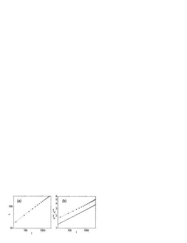
Figure 5: Figure a shows, in a log-log scale, the retreat distance $L$ versus time and its power-law fit $2.75\,t^{0.60}$. Figure b shows, in a log-log scale, the maximum dumbbell height, $h^{max}$ (the empty circles), and the position of the maximum, $x_{1}^{max}$ (the filled circles), versus time, as well as their power-law fits $0.66\,t^{0.21}$ and $0.94\,t^{0.20}$, respectively.

The asymptotic scaling analysis [7] deals with the intermediate stage of the relaxation. Introduce the retreat distance $L(t)=1000-x_{tip}(t)$, where $x_{tip}(t)$ is the maximum abscissa of all points belonging to the interface. One prediction of Ref. [7] is that, at intermediate times, $L(t)\propto t^{3/5}$. Figure 5a shows a very good agreement of this prediction with the simulation result. Additional predictions of asymptotic scaling analysis deal with the time dependence of the maximum dumbbell elevation $h^{max}(t)$, and of the abscissa of the corresponding point of the interface $x^{max}(t)$. Let us introduce a new variable: $x_{1}(x,t)=x_{tip}(t)-x$, the distance along the $x$-axis between the tip of the dumbbell and a point $x$. In particular, $x_{1}^{max}(t)=x_{tip}(t)-x^{max}(t)$. A comparison of the simulation results with the predicted intermediate-time scaling laws $h^{max}(t)\propto x_{1}^{max}(t)\propto t^{1/5}$ is shown in Figure 5b, and again a very good agreement is observed.

To verify the self-similarity of the dumbbell shape in the lobe region, predicted in Ref. [7], we introduce a new function $h(x_{1},t)$ so that $h[x_{1}(x,t),t]=y(x,t)$. Figure 6 shows the spatial profiles of $h$ rescaled to the values of $h^{max}$ versus $x_{1}/x_{1}^{max}$ at three different times. The observed collapse in the lobe region confirms the expected self-similarity.

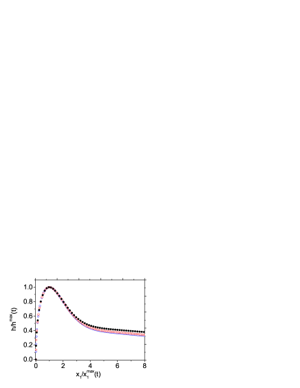
Figure 6: Self-similarity of the lobe. Shown is the shape function $h(x_{1},t)$, rescaled to the maximum dumbbell elevation, versus the coordinate $x_{1}$, rescaled to the abscissa of the maximum, at times $160.3$ (the filled circles), $1000$ (the squares), and $3010$ (the empty circles).

The initial number of nodes in this simulation was 1100, and the smallest spacing in the lobe region was 0.4. With the grid interpolation employed, the time-step parameter $\varepsilon=0.005$ proved sufficiently small to guarantee stability and good accuracy. As the curvature of the interface goes down during the evolution, the required time step increases significantly. It was $1.7\times 10^{-3}$ at $t=0$, $0.22$ at $t=3670$ and increased up to about 10 by the end of the simulation, at $t=48000$. We used the small observed area loss of the bubble for accuracy control. The observed area loss was less then $0.5\%$ for $t<10000$. By the end of the simulation, at $t=48000$, the area loss reached only $2.8\%$.

5 Conclusion

We have developed and tested a new numerical version of the boundary integral method for an exterior Dirichlet problem, which is especially suitable for long and thin domains. The method allows one to significantly reduce the number of the interfacial nodes. The new method was successfully tested in a numerical investigation of the shape relaxation, by surface tension, of a long and thin bubble, filled with an inviscid fluid and immersed in a viscous fluid in a Hele-Shaw cell. Here we confirmed the recent theoretical predictions on the self-similarity and dynamic scaling behavior during an intermediate stage of the bubble dynamics.

References

- [1] J.S. Langer, in Chance and Matter, edited by J. Souletie, J. Vannimenus, and R. Stora, Elsevier, Amsterdam, 1987.
- [2] D. Bensimon, L.P. Kadanoff, S.D. Liang, B.I. Shraiman, C. Tang, Viscous flow in two dimensions, Rev. Mod. Phys. 58 (1986) 977-999.
- [3] D.A. Kessler, J. Koplik, H. Levine, Pattern selection in fingered growth phenomena, Adv. Physics 37 (1988) 255-339.
- [4] J. Casademunt, F.X. Magdaleno, Dynamics and selection of fingering patterns. Recent developments in the Saffman-Taylor problem, Phys. Rep. 337 (2000) 1-35.
- [5] J. Casademunt, Viscous fingering as a paradigm of interfacial pattern formation: Recent results and new challenges, Chaos 14 (2004) 809-824.
- [6] M. Conti, A. Lipshtat, B. Meerson, Scaling anomalies in the coarsening dynamics of fractal viscous fingering patterns, Phys. Rev. E 69 (2004) 031406 (1-4).
- [7] A. Vilenkin, B. Meerson, P.V. Sasorov, Scaling and self-similarity in an unforced flow of inviscid fluid trapped inside a viscous fluid in a Hele-Shaw cell, Phys. Rev. Lett. (submitted).
- [8] P. Constantin, M. Pugh, Global solutions for small data to the Hele-Shaw Problem, Nonlinearity 6 (1993) 393-415.
- [9] The damping rates of small sinusoidal perturbations of circular and flat interfaces are given by the zero-flow-rate limit of Eq. (11) of Ref. [20] (for the circular interface) and Eq. (10) of Ref. [21] (for the flat interface).
- [10] T. Y. Hou, J.S. Lowengrub, M.J. Shelley, Boundary integral methods for multicomponent fluids and multiphase materials, J. Comput. Phys. 169 (2001) 302-362.
- [11] W.-S. Dai, L.P. Kadanoff, S.M. Zhou, Interface dynamics and the motion of complex singularities, Phys. Rev. A 43 (1991) 6672-6682.
- [12] S. Tanveer, Surprises in Viscous Fingering, J. Fluid Mech. 409 (2000) 273-308.
- [13] R. Folch, J. Casademunt, A. Hernandez-Machado, L. Ramirez-Piscina, Phase-field model for Hele-Shaw flows with arbitrary viscosity contrast. I. Theoretical approach, Phys. Rev. E 60 (1999) 1724-1733.
- [14] R. Folch, J. Casademunt, A. Hernandez-Machado, L. Ramirez-Piscina, Phase-field model for Hele-Shaw flows with arbitrary viscosity contrast. II. Numerical study, Phys. Rev. E 60 (1999) 1734-1740.
- [15] K. Glasner, A diffuse inerface approach to Hele-Shaw flow, Nonlinearity 16 (2003) 49-66.
- [16] A. Tikhonov, A. Samarskii, Equations of Mathematical Physics, Pergamon Press, Oxford, 1963.
- [17] A. Greenbaum, L. Greengard, G.B. McFadden, Laplace’s equation and the Dirichlet-Neumann map in multiply connected domains, J. Comput. Phys. 105 (1993) 267-278.
- [18] S.G. Mikhlin, Integral Equations, London, Pergamon, 1957.
- [19] J.T. Beale, T.Y. Hou, J.S. Lowengrub, On the well-posedness of two fluid interfacial flows with surface tension, in Singularities in Fluids, Plasmas and Optics, edited by R. Caflish and G. Papanicolaou, NATO Adv. Sci. Inst. Ser. A, Kluwer Academic, Amsterdam, 1993, p. 11.
- [20] L. Paterson, Radial fingering in a Hele Shaw cell, J. Fluid Mech. 113 (1981) 513-529.
- [21] P.G. Saffman, G.I. Taylor, The penetration of a fluid into a porous medium or Hele-Shaw cell containing a more viscous liquid, Proc. R. Soc. London, Ser. A 245 (1958) 312-329.