A Review of Recent Studies of Geographical Scale-Free Networks

Abstract

The scale-free (SF) structure that commonly appears in many complex networks is one of the hot topics related to social, biological, and information sciences. The self-organized generation mechanisms are expected to be useful for efficient communication or robust connectivity in socio-technological infrastructures. This paper is the first review of geographical SF network models. We discuss the essential generation mechanisms to induce the structure with power-law behavior and the properties of planarity and link length. The distributed designs of geographical SF networks without the crossing and long-range links that cause the interference and dissipation problems are very important for many applications such as in the Internet, power-grid, mobile, and sensor systems.

I Introduction

As a breakthrough in network science Buchnan02 , it has been found Albert02 that many real systems of social, technological, and biological origins have the surprisingly common topological structure called small-world (SW) Watts98 and scale-free (SF) Barabasi99 . The structure is characterized by the SW properties that the average path length over all nodes (vertices) is short as similar to that in random graphs, and that the clustering coefficient, defined by the average ratio of the number of links (edges) connecting to its nearest neighbors of a node to the number of possible links between all these nearest neighbors, is large as similar to that in regular graphs. Large clustering coefficient means the high frequency of “the friend of a friend is also his/her friend.” As the SF property, the degree distribution follows a power-law, $P(k)\sim k^{-\gamma}$, $2<\gamma<3$; the fat-tail distribution consists of many nodes with low degrees and a few hubs with very high degrees. Moreover, a proposal of the universal mechanisms Barabasi99 to generate SF networks inspired to elucidate the topological properties. One of the advantage is that SF networks are optimal in minimizing both the effort for communication and the cost for maintaining the connections Cancho03 . Intuitively, SF network is positioned between star or clique graph for minimizing the path length (the number of hops or legs) and random tree for minimizing the number of links within the connectivity. Another important property is that SF networks are robust against random failures but vulnerable against the targeted attacks on hubs. This vulnerability called “Achilles’ heel of the Internet” Albert00a frightened us. However the vulnerability is a double-edged sword for information delivery and spreading of viruses, we expect that these properties will be useful for developing efficient and fault-tolerant networks with a defense mechanism based on the protection of hubs. Since the SF structure is at least selected with self-organized manners in social and biological environments, the evolutional mechanisms may give insight to distributed network designs or social managements in communication or business.

On the other hand, in contrast to abstract graphs, many real networks are embedded in a metric space. It is therefore natural to investigate the possibility of embedding SF networks in space. The related applications are very wide in the Internet(routers), power-grids, airlines, mobile communication Hong02 , sensor networks Culler04 , and so on. However most of the works on SF networks were irrelevant to a geographical space. In this paper, focusing on the SF structure found in many real systems, we consider generation rules of geographical networks whose nodes are set on a Euclidean space and the undirected links between them are weighted by the Euclidean distance.

The organization of this paper is as follows. In section 2, we introduce an example that shows the restriction of long-range links in real networks. Indeed, the decay of connection probability for the distance between nodes follows exponential or power-law. In section 3, we review recent studies of geographical SF network models, which are categorized in three classes by the generation rules. We refer to the analytical forms of degree distributions that characterize the SF structure. In section 4, we consider the relations among these models. In addition, we compare the properties of planarity and distance of connections. Finally, in section 5, the summary and further issues are briefly discussed.

II Spatial distribution in real-world networks

The restriction of long-range links has been observed in real networks: Internet at both router and autonomous system (AS) levels obtained by using NETGEO tool to identify the geographical coordinates of 228,265 routers Yook02 . These data suggest that the distribution of link lengths (distance) is inversely proportional to the lengths, invalidating the Waxman’s exponentially decay rule Waxman88 which is widely used in traffic simulations. Other evidence has been reported for the real data of Internet as AS level (7,049 nodes and 13,831 links) compiled by the University of Oregon’s Route Views project, road networks of US interstate highway (935 nodes and 1,337 links) extracted from GIS databases, and flight-connections (187 nodes and 825 links) in a major airline Gastner04 . It has been shown that all three networks have a clear bias towards shorter links to reduce the costs for construction and maintenance, however there exist some differences: the road network has only very short links on the order of 10km to 100km in the sharply decaying distribution, while the Internet and airline networks have much longer ones in the bimodal distribution with distinct peaks around 2000km or less and 4000km. These differences may come from physical constraints in the link cost or the necessaries of long distant direct connections.

As a similar example, we investigate the distributions of link lengths (distances of flights) in Japanese airlines JALANA . The networks consists of 52 nodes (airports) and 961 links (flights) in the Japan AirLines (JAL), 49 nodes and 909 links in the All Nippon Airlines (ANA), and 84 nodes and 1,114 links including the international one. Fig. 1 shows the cumulative number of flights for the decreasing order of length measured by mile. We remark an exponential decay in the domestic flights (red and blue lines in the Fig. 1), while it rather follows a power-law by adding the international flights (green line in the Fig. 1). Note that the distribution of the link lengths is obtained by the differential of the cumulative one and that the decay form of exponential or power-law is invariant.

Thus, link lengths are restricted in real systems, although the distribution may have some various forms as similar to the cases of degree distribution Amaral00 .

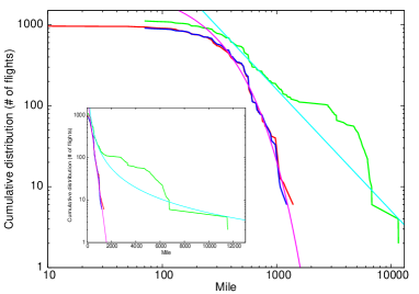
Figure 1: Cumulative number of flights in Japanese airlines. The red, blue, and green lines correspond to domestic flights in JAL, ANA, and that including international flights (Inset: semi-log scale). The magenta and cyan lines guide the estimated functions of exponential and power-law, respectively.

class of SF nets.	generation rule	planar	length	models
with disadvantaged	connection of $(i,t)$ with prob.	$\times$	$\bigcirc$	modulated
long-range links	$\Pi_{i}(t)\sim k_{i}(t)l^{\alpha}$, $\alpha<0$			BA model Manna02 Brunet02
	connection of $(i,j)$ iff	$\times$	$\bigcirc$	geo. threshold
	$(w_{i}+w_{j})h(r_{ij})\geq\theta$			graph Masuda05
embedded on	with randomly assigned $k_{j}$	$\times$	$\bigtriangleup$	Warren et.al. Warren02 ,
a lattice	restricted links			Avraham et.al. Avraham03 Rozenfeld02
	in the radius $Ak_{j}^{1/d}$
by space-filling	triangulation	$\bigcirc$	$\bigtriangleup$	Apollonian
	(geo. attach. pref.)			nets. Zhou04 Zhou05 Doye05
	pref. attach. by	$\times$	$\bigtriangleup$	growing spatial
	selecting edges			SF nets Manna05

Table 1: Summary of geographical SF network models. The symbols $\bigcirc$, $\bigtriangleup$, and $\times$ denote goodness levels for each property.

III Geographical SF network models

We review geographical SF network models in the state-of-the-art. By the generation rules of networks, they are categorized in three classes as shown in Table 1. The generation rules are explained by variations in the balance of minimizing the number of hops between nodes (benefits for transfers) and the link lengths.

In this section, we refer to the generation rules and the power-law behavior only in the essential forms because of the limited pages. The properties of planarity without crossing links and the link lengths will be discussed in the next section.

III.1 SF networks with disadvantaged long-range links

The modulated Barabási-Albert (BA) model Manna02 and the geographical threshold graph Masuda05 belong to the first class: SF networks with disadvantaged long-range links between nodes whose positions are random on a space . They are natural extensions of the previous non-geographical SF network models by the competition of preferential linking based on the degree or weight and the restriction of link length (distance dependence).

III.1.1 Modulated BA model in the Euclidean space

Before explaining the first class, we introduce the well-known BA model Barabasi99 generated by the following rule: growth with a new node at each time and preferential attachment of links to nodes with large degrees (see Fig. 2(a)).

BA-Step 0:

A network grows from an initial $N_{0}$ nodes with $m<N_{0}$ links among them.

BA-Step 1:

At every time step, a new node is introduced and is randomly connected to $m$ previous nodes as follows.

BA-Step 2:

Any of these $m$ links of the new node introduced at time $t$ connects a previous node $i$ with an attachment probability $\Pi^{BA}_{i}(t)$ which is linearly proportional to the degree $k_{i}(t)$ of the $i$th node at time $t$, $\Pi^{BA}_{i}(t)\sim k_{i}(t)$.

The preferential attachment makes a heterogeneous network with hubs. More precisely, the degree distribution $P(k)\sim k^{-3}$ is analytically obtained by using a mean-field approximation Barabasi99 in the continuum approach Albert02 , in which the time dependence of the degree $k_{i}$ of a given node $i$ is calculated through the continuous real variables of degree and time.

Based on a competition between the preferential attachment and the distance dependence of links, the modulated BA model on a space with physical distance has been considered Manna02 . Note that the position of new node is random. The network is grown by introducing at unit rate randomly selected nodes on the Euclidean space (e.g. two-dimensional square area), and the probability of connection is modulated according to $\Pi_{i}(t)\sim k_{i}(t)l^{\alpha}$, where $l$ is the Euclidean distance between the $t$th (birth at time $t$) and the older $i$th nodes, and $\alpha$ is a parameter. The case of $\alpha=0$ is the original BA model Barabasi99 . In the limit of $\alpha\rightarrow-\infty$, only the smallest value of $l$ corresponding to the nearest node will contribute with probability $1$. Similarly, in the limit of $\alpha\rightarrow\infty$, only the furthest node will contribute. Indeed, it has been estimated that the distribution of link lengths follows a power-law $l^{-\delta}$ (long-range links are rare at $\delta>0$), whose exponent is calculated by $\delta=\alpha+d-1$ for all values of $\alpha$ Manna02 .

In the modulated BA model on a one-dimensional lattice (circumference), it has been numerically shown that Brunet02 for $-1<\alpha<0$ the degree distribution is close to a power-law, but for $\alpha<-1$ it is represented by a stretched exponential $P(k)=a\exp(-bk^{\gamma})$, where the parameters $a$, $b$, and $\gamma$ depend on $\alpha$ and $m$, although the SW property Watts98 is preserved at all values of $\alpha$. For the transition from the stretched exponential to the SF behavior, the critical value is generalized to $\alpha_{c}=1-d$ in the embedded $d$-dimensional space Manna02 . More systematic classification in a parameter space of the exponents of degree, distance, and fractal dimension has been also discussed Yook02 .

Other related studies to the form of connection probability $\Pi_{i}\sim k_{i}^{\beta}l^{\alpha}$ are the phase diagram of the clustering properties in the $\alpha$-$\beta$ plane Sen03 , the comparison of the topological properties for the special case of the connection probability proportional to the distance ($\alpha=1$, $\beta=0$) and the inverse distance ($\alpha=-1$, $\beta=0$) Jost02 , the numerical investigation of the scaling for the quantities (degree, degree-degree correlation, clustering coefficient) of the network generated by the connection probability proportional to the degree with the exponential decay of the distance Barthelemy03 , and so on.

III.1.2 Geographical threshold graphs

Th geographical threshold graph Masuda05 is a non-growing network model extended form the threshold SF network model Caldareli02 Masuda04 . It is embedded in the $d$-dimensional Euclidean space with disadvantaged long-range links. We briefly show the analysis of degree distribution.

Let us consider a set of nodes with the size $N$. We assume that each node $i$ is randomly distributed with uniform density $\rho$ in the space whose coordinates are denoted by $x_{1},x_{2},\ldots,x_{d}$, and that it is assigned with a weight $w_{i}\geq 0$ by a density function $f(w)$. According to the threshold mechanism Masuda05 , a pair of node $(i,j)$ is connected iff

$$(w_{i}+w_{j})h(r_{ij})\geq\theta,$$ (1)

where $h(r_{ij})$ is a decreasing function of the distance $r_{ij}>0$ between the nodes, and $\theta$ is a constant threshold.

If $f(w)$ is the Dirac delta function at $w*>0$, then the condition of connection (1) is equivalent to $r_{ij}\geq h^{-1}\left(\frac{\theta}{2w^{*}}\right)\stackrel{{\scriptstyle\rm def}}{{=}}r^{*}$ by using the inverse function $h^{-1}$. This case is the unit disk graph, as a model of mobile and sensor networks, in which the two nodes within the radius $r^{*}$ are connected according to the energy consumption. However, the degree distribution $P(k)$ is homogeneous. We need more inhomogeneous weights.

Thus, if the exponential weight distribution

$$f(w)=\lambda e^{-\lambda w},$$ (2)

and the power-law decay function $h(r_{ij})=(r_{ij})^{-\beta}$, $\beta\geq 0$, are considered, then the degree is derived as a function of weight

$$k(w_{i})=\int_{0}^{\infty}f(w_{j})dw_{j}\int_{(w_{i}+w_{j})/(r_{ij})^{\beta}\geq\theta}\rho dx_{1}\ldots dx_{d}\sim e^{\lambda w_{i}},$$ (3)

after slightly complicated calculations. The second integral in the r.h.s of (3) is the volume of $d$-dimensional hypersphere. As in Refs. Masuda05 Masuda04 , by using the relation of cumulative distributions $\int_{0}^{k(w)}P(k)dk=\int_{-\infty}^{w}f(w^{\prime})dw^{\prime}$, we have

$$P(k)=f(w)\frac{dw}{dk}.$$ (4)

From (3) and (4), we obtain the power-law degree distribution

$$P(k)\sim e^{-2\lambda w}\sim k^{-2}.$$

Note that this result is derived only if the value of $\beta$ is sufficiently small, otherwise the degree distribution has a streched exponential decay or an exponential decay.

On the other hand, for the power-law weight distribution (called Parete distribution in this form)

$$f(w)=\frac{\alpha}{w^{*}}\left(\frac{w^{*}}{w}\right)^{\alpha+1},$$ (5)

we similarly obtain

$$k(w)\sim w^{d/\beta},\;\;P(k)\sim k^{-(1+\alpha\beta/d)}.$$

The exponent $\gamma\stackrel{{\scriptstyle\rm def}}{{=}}1+\alpha\beta/d$ is a variable depends on the parameters $\alpha$ and $\beta$.

Furthermore, we mention a gravity model with $h(r_{ij})=1/\log r_{ij}$. In this case, the condition of connection (1) is rewritten as $w_{i}+w_{j}\geq\theta\log r_{ij}$, and into

$$\frac{W_{i}W_{j}}{(R_{ij})^{\beta}}\geq\theta,$$ (6)

by the variable transformations $W_{i}\stackrel{{\scriptstyle\rm def}}{{=}}e^{w_{i}}$, $W_{j}\stackrel{{\scriptstyle\rm def}}{{=}}e^{w_{j}}$, and $(R_{ij})^{\beta}\stackrel{{\scriptstyle\rm def}}{{=}}(r_{ij})^{\theta}/\theta$. Eq. (6) represents a physical, sociological, or chemical interactions with power-law distance dependence. For the combination of (6) and the weight distributions $f(w)$ in (2) and (5), we can also derive the more complicated forms of $P(k)$. Thus, the choice of $f(w)$ matters for the SF properties in contrast to an approximately constant exponent $\gamma\approx 2$ in the non-geographical threshold graphs Masuda04 without $h(r_{ij})$.

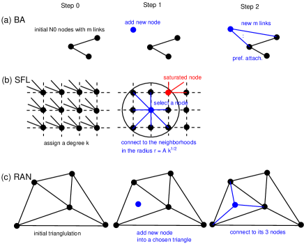
Figure 2: Network generation in each model. The analytically obtained degree distributions for (a)-(c) follow $P(k)\sim k^{-3}$, $P(k)\sim k^{-\gamma}$ with cutoff $k_{c}<K$, and $P(k)\sim k^{-\gamma_{RA}}$, $\gamma_{RA}\sim 3$, respectively.

III.2 SF networks embedded on lattices

The second class is based on the SF networks embedded on regular Euclidean lattices (SFL) accounting for graphical properties Avraham03 Rozenfeld02 . We distinguish this class from the first one, because the position of node is not randomly distributed but well-ordered on a lattice with a scale that gives the minimum distance.

Let us consider a $d$-dimensional lattice of size $R$ with periodic boundary conditions. The model is defined by the following configuration procedures (see Fig. 2(b)) on an assumption of power-law degree distribution.

SFL-Step 0:

To each node on the lattice, assign a random degree $k$ taken from the distribution $P(k)=Ck^{-\lambda}$, $m\leq k\leq K$, $\lambda>2$, (the normalization constant: $C\approx(\lambda-1)m^{\lambda-1}$ for large $K$).

SFL-Step 1:

Select a node $i$ at random, and connect it to its closest neighbors until its connectivity $k_{i}$ is realized, or until all nodes up to a distance,

$$r(k_{i})=Ak_{i}^{1/d},$$ (7)

have been explored: The connectivity quota $k_{j}$ of the target node $j$ is already filled in saturation. Here $A>0$ is a constant.

SFL-Step 2:

The above process is repeated for all nodes.

As in Ref. Avraham03 , we derive the cutoff connectivity. Consider the number of links $n(r)$ entering a node from a surrounding neighborhood of radius $r$, when the lattice is infinite, $R\rightarrow\infty$. The probability of connections between the origin and nodes at distance $r^{\prime}$ is

$$P\left(k>\left(\frac{r^{\prime}}{A}\right)^{d}\right)=\int_{(r^{\prime}/A)^{d}}^{\infty}P(k^{\prime})dk^{\prime}\sim\left\{\begin{array}[]{cc}1&r^{\prime}<A\\ (r^{\prime}/A)^{d(1-\lambda)}&r^{\prime}>A.\end{array}\right.$$

Thus, from $n(r)=\int_{0}^{r}S_{d}r^{\prime d-1}dr^{\prime}\int_{(r^{\prime}/A)^{d}}^{\infty}P(k^{\prime})dk^{\prime}$, we obtain

$$n(r)=V_{d}r^{d}\left\{\left(\frac{A}{r}\right)^{d}\int_{0}^{(r/A)^{d}}kP(k)dk+\int_{(r/A)^{d}}^{\infty}P(k)dk\right\},$$

where $V_{d}=S_{d}/d$ and $S_{d}$ is the volume and the surface area of the $d$-dimensional unit sphere, respectively. The cutoff connectivity is then

$$k_{c}=\lim_{r\rightarrow\infty}n(r)=V_{d}A^{d}\langle k\rangle,$$ (8)

where $\langle k\rangle=\int kP(k)dk$ denotes the average connectivity.

If $A$ is large enough such that $k_{c}>K$, the network can be embedded without cutoff. Otherwise, by substituting (8) into (7), the cutoff connectivity $k_{c}$ implies a cutoff length

$$\xi=r(k_{c})=(V_{d}\langle k\rangle)^{1/d}A^{2}.$$ (9)

The embedded network displays the original (power-law) distribution up to length scale $\xi$ and repeats, statistically, at length scales larger than $\xi$.

Whenever the lattice is finite, $R<\infty$, the number of nodes is finite, $N\sim R^{d}$, which imposes a maximum connectivity,

$$K\sim mN^{1/(\lambda-1)}\sim R^{d/(\lambda-1)},$$ (10)

where the first approximation is obtained from $\int_{K}^{\infty}P(k)dk=\left[\frac{C}{1-\lambda}k^{1-\lambda}\right]_{K}^{\infty}=1/N$. From (7) and (10), a finite-size cutoff length is

$$r_{max}=r(K)\sim AR^{1/(\lambda-1)}.$$ (11)

These three length scales, $R$, $\xi$, $r_{max}$, determine the nature of networks. If the lattice is finite, then the maximum connectivity $K$ is attained only if $r_{max}<\xi$. Otherwise ($r_{max}>\xi$), the cutoff $k_{c}$ is imposed. As long as $\min(r_{max},\xi)\ll R$, the lattice size $R$ imposes no serious restrictions. Otherwise ($\min(r_{max},\xi)\geq R$), finite-size effects bounded by $R$ becomes important. In this regime, the simulation results Avraham03 Rozenfeld02 have also shown that for larger $\lambda$ the network resembles the embedding lattice because of the rare long-range links, while the long-range links becomes noticeable as $\lambda$ decreases.

Concurrently with the above work, Warren et al. Warren02 have proposed a similar embedding algorithm in a two-dimensional lattice, however the number of nodes in each circle is equal to the connectivity without cutoff. Thus, the main difference in their approaches is that a node can be connected to as many of its closest neighbors as necessary, until its target connectivity is fulfilled.

In addition, Ref. Moukarzel02 has discussed the shortest paths on $d$-dimensional lattices with the addition of an average of $p$ long-range bonds (shortcuts) per site, whose length $l$ is distributed according to $P_{l}\sim l^{-\mu}$.

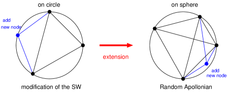
Figure 3: Growing networks with geographical attachment preference. The blue node and links are newly added.

III.3 Space-filling networks

The third class is related to the space-filling packing in which a region is iteratively partitioned into subregions by adding new node and links.

III.3.1 Growing small-world networks

Let us consider the growing network with geographical attachment preference Ozik04 as a modification of the SW model Watts98 . In this network, from an initial configuration with $m+1$ completely connected nodes on the circumference of a circle, at each subsequent time step, a new node is added in an uniform-randomly chosen interval, and connects the new node to its $m$ nearest neighbors w.r.t distance along the circumference. Fig. 3 (left) illustrates the case of $m=2$. We denote $n(k,N)$ as the number of nodes with degree $k$ when the size (or time) is $N$. At time $N$, a new node with degree $m$ is added to the network, and if it connects to a preexisting node $i$, then the degree is updated by $k_{i}\rightarrow k_{i}+1$ with the equal probability $m/N$ to all nodes because of the uniform randomly chosen interval.

Thus, we have the following evolution equation,

$$n(k,N+1)=\left(1-\frac{m}{N}\right)n(k,N)+\frac{m}{N}n(k-1,N)+\delta_{k,m},$$

where $\delta_{k,m}$ is the Kronecker delta. Note that considering such equation for the average number of nodes with $k$ links at time $N$ is called “rate-equation approach,” while considering the probability $p(k,t_{i},t)$ that at time $t$ a node $i$ introduced at time $t_{i}$ has a degree $k$ is called “master equation approach” Albert02 .

When $N$ is sufficient large, $n(k,N)$ can be approximated as $NP(k)$. In the term of degree distribution, we obtain

$$P(k)=\frac{1}{m+1}\left(\frac{m}{m+1}\right)^{k-m},$$

for $k\gg m$ ($P(k)=0$ for $k<m$), although it is not a power-law.

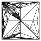
(a) RAN

(b) Deterministic AN

Figure 4: Apollonian Networks: (a) Random AN generated from an initial triangulation of square and (b) Deterministic AN generated from an initial triangle of back lines. The red and blue lines are added links at the first and second steps, respectively.

III.3.2 Apollonian networks

The growing small-world networks model Ozik04 can be extended from polygonal divisions on a circle to polyhedral divisions on a sphere as shown in Fig. 3. We should remark the extended model becomes a planar graph, when each node on the surface is projected onto a plane such as from a Riemannian sphere. It is nothing but a random Apollonian network (RAN) Zhou04 Zhou05 , and also the dual version of Apollonian packing for space-filling disks into a sphere Doye05 , whose hierarchical structure is related to the SF network formed by the minima and transition states on the energy landscape Doye02 . The power-law degree distribution has been analytically shown in the RAN Zhou04 Zhou05 . To derive the distribution $P(k)$, we consider the configuration procedures of RAN as follows (see Fig. 2(c)).

RAN-Step 0:

Set an initial triangulation with $N_{0}$ nodes.

RAN-Step 1:

At each time step, a triangle is randomly chosen, and a new node is added inside the triangle.

RAN-Step 2:

The new node is connected to its three nodes of the chosen triangle.

RAN-Step 3:

The above processes in Steps 1 and 2 are repeated until reaching the required size $N$ .

Since the probability of connection to a node is higher as the number of its related triangles is larger, it is proportional to its degree as the preferential attachment. Thus, we have the following rate-equation

$$n(k+1,N+1)=\frac{k}{N_{\triangle}}n(k,N)+\left(1-\frac{k+1}{N_{\triangle}}\right)n(k+1,N),$$ (12)

where the number of triangles $N_{\triangle}$ (at the grown size or time $N$) is defined as $N_{\triangle}=2(N-4)+4$ for an initial tetrahedron, and $N_{\triangle}=2(N-3)+1$ for an initial triangle, etc.

In the term of $P(k)\approx n(k,N)/N$, Eq. (12) can be rewritten as

$$(N+1)P(k+1)=\frac{NkP(k)}{N_{\triangle}}+NP(k+1)-\frac{N(k+1)P(k+1)}{N_{\triangle}}.$$

By the continuous approximation, we obtain the solution $P(k)\sim k^{-\gamma_{RA}}$ with $\gamma_{RA}=(N_{\triangle}+N)/N\approx 3$ for large $N$. Fig. 4 (a) shows an example of RAN.

Moreover, in the deterministic version Doye05 Andrade05 , analytical forms of the power-law degree distribution $P(k)$, clustering coefficient $c_{i}$, and the degree-degree correlation $k_{nn}(k)$ can be derived Doye05 , since the calculations are easier in the recursive structure without randomness into subregions as shown in Fig 4 (b). Here, $k_{nn}(k)$ is defined by the the average degree of the nearest neighbors of nodes with degree $k$. It has been observed in technological or biological networks and in social networks that there exists two types of correlations, namely disassortative and assortative mixings Newman03b . These types of networks tend to have connections between nodes with low-high degrees and with similar degrees, respectively. The RAN shows the disassortative mixing Doye05 .

Similarly, the analytical forms in the high-dimensional both random Zhang05b Gu05 and deterministic Zhang05c Apollonian networks have been investigated by using slightly different techniques. They are more general space-filling models embedded in a high-dimensional Euclidean space, although the planarity is violated.

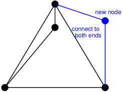
(a) growing SW network

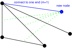
(b) growing spatial SF network

Figure 5: SW and SF networks generated by randomly selecting edges.

III.3.3 SF networks generated by selecting edges

Another modification of the growing SW networks Ozik04 is based on random selection of edges Zhang05a Manna05 . We classify them in the relations to the partitions of interval or region as mentioned in 3.3.1 and a Voronoi diagram. The following two models give typical configurations (see Fig. 5).

The growing SW network generated by selecting edges Zhang05a is constructed as follows. Initially, the network has three nodes, each with degree two. As shown in Fig. 5(a), at each time step, a new node is added, which is attached via two links to both ends of one randomly chosen link that has never been selected before. The growth process is repeated until reaching the required size $N$. Since all nodes have two candidates of links for the selection at each time, an exponential degree distribution has been analytically obtained. If the multi-selection is permitted for each link, it follows a power-law. The difference in configuration procedures for RAN is that, instead of triangulation with adding three links, two links are added at each step. We assume that the position of added node is random (but the nearest to the chosen link) on a metric space, although only the topological properties are discussed in the original model Zhang05a .

In the growing spatial SF network Manna05 on a two-dimensional space, $m$ links whose center points are nearest to an added new node (as guided by the dashed lines in Fig. 5 (b)) are chosen at each time step. Both end nodes of the nearest link(s) have an equal probability of connection. If a Voronoi region Imai00 Okabe00 for the center points of links is randomly chosen for the position of new node in the region , the selection of a link is uniformly random, therefore the probability of connection to each node is proportional to its degree. Then, we can analyze the degree distribution. Note that any point in the Voronoi region is closer to the center (called generator point) belong in it than to any other centers.

For the case of $m=1$ as a tree, the number of node with degree $k$ is evolved in the rate-equation

$$n(k,t+1)=n(k,t)+\frac{(k-1)}{2t}n(k-1,t)-\frac{k}{2t}n(k,t)+\delta_{k,1},$$ (13)

where $n(k,t)$ denotes the number of nodes with degree $k$, and $2t$ is the total degree at time $t$.

In the term of degree distribution $P(k,t)\approx n(k,t)/t$ at time $t$, Eq. (13) is rewritten as

$$(t+1)P(k,t+1)-tP(k,t)=$$

$$\frac{1}{2}\left[(k-1)P(k-1,t)-kP(k,t)\right]+\delta_{k,1}.$$

At the stationary value independent of time $t$, we have

$$P(k)=\frac{1}{2}\left[(k-1)P(k-1)-kP(k)\right]+\delta_{k,1}.$$

From the recursion formula and $P(1)=2/3$, we obtain the solution

$$P(k)=\frac{k-1}{k+2}P(k-1)=\frac{4}{k(k+1)(k+2)}\sim k^{-3}.$$

IV Relations among the models

We discuss the relations among the independently proposed models. Remember the summary of the geographical SF network models in Table 1.

The first class is based on a combination of the preferential attachment or the threshold mechanism and the penalty of long-range links between nodes whose position is random, while the second one is on embedding the SF structure with a given power-law degree distribution in a lattice. Since the assigned degree to each node can be regarded as a fitness Albert02 , the SFL is considered as a special case of the fitness model Caldareli02 embedded on a lattice. In contrast, the penalty of age or distance dependence of each node can be regarded as a non-fitness in general term. If we neglect the difference of penalties, this explanation bridges the modulated BA Manna02 Brunet02 , SFL Avraham03 Rozenfeld02 , and aging models Dorogovtsev00 with a generalized fitness model. The crucial difference is the positioning of nodes: one is randomly distributed on a space and another is well-ordered on a lattice with the minimum distance between nodes. Moreover, the weight in the threshold graphs Masuda05 Masuda04 is corresponded to a something of fitness, however the deterministic threshold and the attachment mechanisms should be distinguished in the non-growing and growing networks. We also remark that, in the third class, the preferential attachment is implicitly performed, although the configuration procedures are more geometric based on triangulation Zhou04 Zhou05 Doye05 or selecting edges Manna05 . In particular, the position of nodes in the Apollonian networks is given by the iterative subdivisions (as neither random nor fixed on lattice), which may be related to territories for communication or supply management in practice.

Next, we qualitatively compare the properties of planarity without crossing links and link lengths. We emphasize that the planarity is important and natural requirement to avoid the interference of beam (or collision of particles) in wireless networks, airlines, layout of VLSI circuits, vas networks clinging to cutis, and other networks on the earth’s surface, etc Zhou05 .

In the modulated BA models and the geographical threshold graphs, long-range links are restricted by the strong constraints with decay terms, however crossing links may be generated. There exist longer links from hubs in the SFL, because such nodes have large number of links however the positions of nodes are restricted on a lattice; the density of nodes is constant, therefore they must connect to some nodes at long distances. More precisely, it depends on the exponent $\lambda$ of power-law degree distribution as mentioned in the subsection 3.2. In addition, the planarity is not satisfied by the crossing between the lattice edges and the short-cuts. On the other hand, RAN has both good properties of the planarity and averagely short links. However, in a narrow triangle region, long-range links are partially generated as shown in Fig. 4. Similarly, the SF networks generated by selecting edges may have long-range links as shown in Fig. 5 (b): the chosen end point for connection is long away from the newly added node at a random position, even though the selected edges have the nearest centers.

V Conclusion

In this review of geographical SF network models, we have categorized them in three classes by the generation rules: disadvantaged long-range links, embedding on a lattice, and space-filling. We have shown that these models have essential mechanisms to generate power-law degree distributions, whose analytical forms can be derived on an assumption of the restricted link lengths as consistent with real data. Furthermore, the basic topological properties of the planarity and link length have been discussed for each model. In particular, the geographical threshold graphs and the RAN are attractive because of the tunable exponent $\gamma$ of $P(k)\sim k^{-\gamma}$ or the locality related to the unit disk graphs, and the planarity of network on the heterogeneous positioning of nodes. However, they have drawbacks of crossing and long-range links, respectively. To avoid long-range links, an improvement by the combination of RAN and Delaunay triangulation based on diagonal flipping Imai00 Okabe00 is considering Hayashi05 .

We have grasped several configuration procedures of geographical SF networks and discussed the above properties, however these are still at the fundamental level. We must consider further issues, for example,

• Quantitative investigation of the topological properties including diameter of network, clustering coefficient, degree-degree correlation, and betweenness centrality (related to congestion of information flow), etc.

• Analysis of dynamics for the traffic and the fault-tolerance, especially in disaster or emergent environment.

• Positioning of nodes with aggregations according to a population density in the evolutional and distributed manners.

We will progress to the next stage from the observation of real networks to the development of future networks. The distributed design and management will be usefully applied to many socio-technological infrastructures.

References

- (1) Buchanan, M.: Nexus: Small Worlds and the Groundbreaking Science of Networks, Norton & Company, Inc., 2002.
- (2) Albert, R., and Barabási, A.-L.: Statistical Mechanics of Complex Networks, Rev. Mod. Phys., Vol. 74, pp. 47-97, (2002).
- (3) Watts, D.J., and Strogatz, S.H.: Collective dynamics of small-world networks, Nature, Vol. 393, pp. 440, (1998).
- (4) Barabási, A.-L., Albert, R., and Jeong, H.: Mean-field theory for scale-free random networks, Physica A, Vol. 272, pp. 173-187, (1999).
- (5) Cancho, R.F.i, and Solé, R.V.: Optimization in Complex Networks, In Pastor-Satorras, R., Rubi, M., and Diaz-Guilera, A. (eds.) Statistical Mechanics of Complex Networks, Chapter 6, pp. 114-126, (2003).
- (6) Albert, R., Jeong, H., and Barabási, A.-L.: Error and attack tolerance of complex networks, Nature, Vol. 406, pp. 378-382, (2000).
- (7) Hong, X., Xu, K., and Gerla, M.: Scalable Routing Protocols for Mobile Ad Hoc Networks, IEEE Network, pp. 11-21, July/August (2002).
- (8) Culler, D.E., and Mulder, H.: Smart Sensors to Network the World, Scientific American, pp. 84-91, June (2004).
- (9) Yook, S.-H., Jeong, H., and Barabási, A.-L.: Modeling the Internet’s large-scale topology, PNAS, Vol. 99, No. 21, pp. 13382-13386, (2002).
- (10) Waxman, B.M.: Routing of multipoint connections, IEEE Journal of Selected Areas in Communications, Vol. 6, pp. 1617-1622, (1988).
- (11) Gastner, M.T., and Newman, M.E.J.: The spatial structure of networks, arXiv:cond-mat/0407680, (2004).
- (12) JAL domestic flight schedule and service guide, ANA group flight schedule, April-May 2005.
- (13) Amaral, L.A., Scala, A., Barthélémy, M., and Stanley, H.E.: Classes of behavior of small-world networks, PNAS, Vol. 97, pp. 11149, (2000).
- (14) Manna, S.S., and Parongama, S.: Modulated scale-free networks in Euclidean space, Phys. Rev. E, Vol. 66, pp. 066114, (2002).
- (15) Sen, P., and Manna, S.S.: Clustering properties of a generalized critical Euclidean network, Phys. Rev. E, Vol. 68, pp. 026104, (2003).
- (16) Jost, J., and Joy, M.P.: Evolving networks with distance preferences, Phys. Rev. E, Vol. 66, pp. 036126, (2002).
- (17) Barthélemy, M.: Crossover from scale-free to spatial networks, Europhys. Lett., Vol. 63, No. 6, pp. 915-921, (2003).
- (18) Masuda, N., Miwa, H., and Konno, N.: Geographical threshold graphs with small-world and scale-free properties, Phys. Rev. E, Vol. 71, pp. 036108, (2005).
- (19) Xulvi-Brunet, R., and Sokolov, I.M.: Evolving networks with disadvantaged long-range connections, Phys. Rev. E, Vol. 66, pp. 026118, (2002).
- (20) Caldareli, G, Capocci, A., Rios, P.DeLos, Muñoz, M.A.: Scale-free Networks from Varying Vertex Intrinsic Fitness, Physical Review Letters, Vol. 89, pp. 258702, (2002).
- (21) Masuda, N., Miwa, H., and Konno, N.: Analysis of scale-free networks based on a threshold graph with intrinsic vertex weights, Phys. Rev. E, Vol. 70, pp. 036124, (2004).
- (22) ben-Avraham, D., Rozenfeld, A.F., Cohen, R., and Havlin, S.: Geographical embedding of scale-free networks, Physica A, Vol. 330, pp. 107-116, (2003).
- (23) Rozenfeld, A.F., Cohen, R., ben-Avraham, D., and Havlin, S.: Scale-Free Networks on Lattices, Phys. Rev. Lett., Vol. 89, pp. 218701, (2002).
- (24) Warren, C.P., Sander, L.M., and Sokolov,I.M.: Geography in a scale-free network model, Phys. Rev. E, Vol. 66, pp. 056105, (2002).
- (25) Moukarzel, C.F., and Argollo de Menzes, M.: Shortest paths on systems with power-law distributed long-range connections, Phys. Rev. E, Vol. 65, pp. 056709, (2002).
- (26) Ozik, J., Hunt, B.R., and Ott, E.: Growing networks with geographical attachment preference: Emergence of small worlds, Phys. Rev. E, Vol. 69, pp. 026108, (2004).
- (27) Zhou, T., Yan, G., Zhou, P.-L., Fu, Z.-Q., and Wang, B.-H.: Random Apollonian Networks, arXiv:cond-mat/0409414, (2004).
- (28) Zhou, T., Yan, G., and Wang, B.-H.: Maximal planar networks with large clustering coefficient and power-law degree distribution, Phys. Rev. E, Vol. 71, pp. 046141, (2005).
- (29) Doye, J.P.K., and Massen, C.P.: Self-similar disk packings as model spatial scale-free networks, Phys. Rev. E, Vol. 71, pp. 016128, (2005).
- (30) Doye, J.P.K.: Network Topology of a Potential Energy Landscape: A Static Scele-Free Network, Phys. Rev. Lett., Vol. 88, pp. 238701, (2002).
- (31) Andrade, Jr., J.S., Herrmann, H.J., Andrade, R.F.S., and da Silva, L.R.: Apollonian Networks: Simultaneously Scale-Free, Small World, Euclidiean, Space Filling, and with Matching Graphs, Phys. Rev. Lett., Vol. 94, pp. 018702, (2005).
- (32) Newman, M.E.J.: Mixing patterns in networks, Phys. Rev. E, Vol. 67, pp. 026126, (2003).
- (33) Zhang, Z., Rong, L., and Comellas, F.: High dimensional random Apollonian networks, arXiv:cond-mat/0502591, (2005).
- (34) Gu. Z.-M., Zhou, T., Wang, B.-H., Yan, G., Zhu, C.-P., and Fu, Z.-Q.: Simplex triangulation induced scale-free networks, arXiv:cond-mat/0505175, (2005).
- (35) Zhang, Z., Comellas, F., Fertin, G., and Rong, L.: High Dimensional Apollonian Networks, arXiv:cond-mat/0503316, (2005).
- (36) Zhang, Z., and Rong, L.: Growing Small-World Networks Generated by Attaching to Edges, arXiv:cond-mat/0503637, (2005).
- (37) Mukherjee, G., and Manna, S.S.: Growing spatial scale-free graphs by selecting local edges, arXiv:cond-mat/0503697, (2005).
- (38) Imai, K: Structures of Triangulations of Points, IEICE Trans. on Inf. and Syst., Vol. 83-D, No.3, pp. 428–437, (2000).
- (39) Okabe, Boots, Sugihara, and Chiu, S.N.: Spatial Tessellations, 2nd ed., John Wiley, 2000.
- (40) Dorogovtsev, S.N., and Mendes, J.F.F.: Evolution of networks with aging of sites, Phys. Rev. E, Vol. 62, pp. 1842, (2000).
- (41) Hayashi, Y., and Matsukubo, J.: Scale-free networks on a geographical planar space for efficient ad hoc communication, Proc. of the Int. Symp. on Nonlinear Theory and Its Applications, pp.118-121, (2005).