Including of triple excitations in the relativistic coupled-cluster formalism and calculation of Na properties.

Abstract

A practical high-accuracy relativistic method of atomic structure calculations for univalent atoms is presented. The method is rooted in the coupled-cluster formalism and includes non-perturbative treatment of single and double excitations from the core and single, double and triple excitations involving valence electron. Triple excitations of core electrons are included in the fourth-order of many-body perturbation theory. In addition, contributions from the disconnected excitations are incorporated. Evaluation of matrix elements includes all-order dressing of lines and vertices of the diagrams. The resulting formalism for matrix elements is complete through the fourth order and sums certain chains of diagrams to all orders. With the developed method we compute removal energies, magnetic-dipole hyperfine-structure constants $A$ and electric-dipole amplitudes. We find that the removal energies are reproduced within 0.01-0.03% and the hyperfine constants of the $3s_{1/2}$ and $3p_{1/2}$ states with a better than 0.1% accuracy. The computed dipole amplitudes for the principal $3s_{1/2}-3p_{1/2;3/2}$ transitions are in an agreement with 0.05%-accurate experimental data.

I Introduction

This work is aimed at designing a practical ab initio atomic-structure method capable of reaching accuracy at the level of 0.1% for properties of heavy univalent many-electron atomic systems. The improved accuracy is required, for example, for a refined interpretation of atomic parity violation (APV) with atomic Cs Khriplovich (1991); Bouchiat and Bouchiat (1997); Wood et al. (1997) and planned experiment with Ba⁺ Koerber et al. (2003). At present namely the accuracy of solving the basic correlation problem is the limiting factor in the APV probe of “new physics” beyond the standard model of elementary particles. In addition, it is anticipated that the improved accuracy would unmask so far untested contributions from quantum electrodynamics (QED) in heavy neutral many-electron systems Sapirstein and Cheng (2003).

Here we report developing a many-body approach based on the coupled-cluster (CC) formalism Coester and Kümmel (1960); Čìžek (1966). In the CC formalism the many-body contributions to wave function are lumped into a hierarchy of multiple (single, double, …) particle-hole excitations from the lowest-order state. Due to a computational complexity, previous relativistic CC-type calculations Blundell et al. (1989, 1991); Eliav et al. (1994); Avgoustoglou and Beck (1998); Safronova et al. (1998); Safronova et al. (1999a) for univalent atoms were limited to single- and double excitations. Triple excitations were treated only in an approximate semi-perturbative fashion  Blundell et al. (1989, 1991); Safronova et al. (1998); Safronova et al. (1999a); Gopakumar et al. (2001); Chaudhuri et al. (2003). Compared to these previous calculations, here we fully include valence triple excitations in the CC formulation; we will designate our approximation as CCSDvT method. Further, compared to calculations by Notre Dame group, here we also incorporate a subset of so-called disconnected excitations (non-linear CC terms). For sodium atom, such non-linear CC terms were previously included in Ref. Eliav et al. (1994) and in non-relativistic calculations Salomonson and Ynnerman (1991). Finally, in calculations of matrix elements we include CC-dressing of lines and vertices Derevianko and Porsev (2005) and we also directly compute complementary fourth-order diagrams (mainly due to core triple excitations). The resulting formalism for matrix elements is complete through the fourth-order of many-body perturbation theory (MBPT) and also subsumes certain chains of diagrams to all orders.

As a first application of our method, we carry out numerical calculations for atom of sodium. Sodium (11 electrons) has an electronic structure similar to cesium (55 electrons), but it is not as demanding computationally. By computing properties of Na atom we observe that a simultaneous treatment of triple and disconnected quadruple excitations is important for improving theoretical accuracy, as the two effects tend to partially cancel each other. We compute removal energies, magnetic-dipole hyperfine-structure (HFS) constants $A$ and electric-dipole amplitudes for the principal $3s_{1/2}-3p_{j}$ transitions. We find that the removal energies are reproduced within 0.01-0.03% and the HFS constants of the $3s$ and $3p_{1/2}$ states with a better than 0.1% accuracy. The computed dipole amplitudes are in a perfect agreement with the 0.05%-accurate experimental data. However, our result for the HFS constant of the $3p_{3/2}$ state disagrees with the most accurate experimental values Yei et al. (1993); Gangrsky et al. (1998) by  1%, while agreeing with less accurate measurements Krist et al. (1977); Arimondo et al. (1977).

The paper is organized as follows. First we discuss generalities of the coupled-cluster formalism and many-body perturbation theory in Sec. II. Explicit CCSDvT equations and analytical expressions for energies, matrix elements, and normalization corrections are presented in Section III. In Sec. IV we tabulate and analyze the results of numerical calculations of properties of sodium atom. Finally, we draw conclusions in Sec. V. Unless specified otherwise, atomic units $|e|=\hbar=m_{e}=4\pi\varepsilon_{0}\equiv 1$ are used throughout.

II Generalities

In this Section we recapitulate relevant formulas and ideas of atomic many-body perturbation theory (MBPT) and the coupled-cluster formalism for systems with one valence electron outside the closed-shell core.

II.1 Atomic Hamiltonian and conventions

The Hamiltonian of an atomic system may be represented as

$$H=\left(\sum_{i}\,h_{\rm nuc}(\mathbf{r}_{i})+\sum_{i}\,U_{\rm DHF}(\mathbf{r}_{i})\right)+\left(\frac{1}{2}\sum_{i\neq j}\frac{1}{r_{ij}}-\sum_{i}\,U_{\rm DHF}(\mathbf{r}_{i})\right)\,,$$ (1)

where $h_{\rm nuc}$ is the Dirac Hamiltonian including kinetic energy of electron and its interaction with the nucleus, $U_{\rm DHF}$ is the Dirac-Hartree-Fock (DHF) potential, and the last term represents the residual Coulomb interaction between electrons. To reduce the number of MBPT diagrams, we employ frozen-core (or $V^{N-1}$) DHF potential Kelley (1969). The single-particle orbitals $\varphi_{i}$ and energies $\varepsilon_{i}$ are found from the set of DHF equations,

$$\left(h_{\rm nuc}+U_{\rm DHF}\right)\varphi_{i}=\varepsilon_{i}\varphi_{i}\,.$$ (2)

The Hamiltonian in the second quantization reads (omitting common energy offset)

$$H=H_{0}+G=\sum_{i}\varepsilon_{i}N[a_{i}^{\dagger}a_{i}]+\frac{1}{2}\sum_{ijkl}g_{ijkl}N[a^{\dagger}_{i}a^{\dagger}_{j}a_{l}a_{k}]\,,$$ (3)

where operators $a_{i}$ and $a_{i}^{\dagger}$ are annihilation and creation operators, and $N[\cdots]$ stands for a normal product of operators with respect to the core quasi-vacuum state $|0_{c}\rangle$. Labels $i,j,k$ and $l$ range over all possible single-particle orbitals. In the following we will employ a labeling convention where letters $a,b,c$ are reserved for core orbitals, indices $m,n,r,s$ label virtual states, and letters $v$ and $w$ designate valence orbitals. In this convention valence orbitals are classified as the virtual orbitals. In Eq. (3), the quantities $g_{ijkl}$ are two-body Coulomb matrix elements

$$g_{ijkl}=\int d^{3}\mathbf{r}\int d^{3}\mathbf{r}^{\prime}\varphi_{i}^{\dagger}(\mathbf{r})\varphi_{j}^{\dagger}(\mathbf{r}^{\prime})\frac{1}{\left|\mathbf{r}-\mathbf{r}^{\prime}\right|}\varphi_{k}(\mathbf{r})\varphi_{l}(\mathbf{r}^{\prime})\,.$$ (4)

Notice the absence of the one-body contribution of $G$ in the second-quantized Hamiltonian, Eq. (3); this simplifying feature is due to the employed $V^{N-1}$ approximation and leads to a greatly reduced number of terms in the CC equations.

In MBPT the first part of the Hamiltonian (3) is treated as the lowest-order Hamiltonian $H_{0}$ and the residual Coulomb interaction $G$ as a perturbation. In the lowest order the atomic wave function with the valence electron in an orbital $v$ reads $|\Psi_{v}^{(0)}\rangle=a^{\dagger}_{v}|0_{c}\rangle$. Further the wave operator $\Omega$ is introduced; it promotes this lowest-order state to the exact many-body wave function

$$|\Psi_{v}\rangle=\Omega\,|\Psi_{v}^{(0)}\rangle.$$ (5)

In the conventional order-by-order MBPT, a perturbative expansion for operator $\Omega$ is built in powers of residual interaction $G$ resulting in a hierarchy of approximations for correlated energies and wave-functions.

II.2 Coupled-cluster method

One of the mainstays of practical application of MBPT is an assumption of convergence of series in powers of the perturbing interaction. Sometimes the convergence is poor and then one sums certain classes of diagrams to “all orders” using iterative techniques. The coupled-cluster formalism is one of the most popular all-order methods. The key point of the CC method is the introduction of an exponential ansatz for the wave operator Lindgren and Morrison (1986)

$$\Omega=N[\exp(K)]=1+K+\frac{1}{2!}N[K^{2}]+\ldots\,,$$ (6)

where the cluster operator $K$ is expressed in terms of connected diagrams of the wave operator $\Omega$. The operator $K$ is naturally broken into cluster operators $\left(K\right)_{n}$ combining $n$ simultaneous excitations of core and valence electrons from the reference state $|\Psi_{v}^{(0)}\rangle$ to all orders of MBPT

$$K=\sum_{n}^{\textrm{total number of electrons}}\left(K\right)_{n}=S+D+T+\cdots,$$ (7)

i.e., $K$ is separated into singles ($S\equiv\left(K\right)_{1}$), doubles ($D\equiv\left(K\right)_{2}$), triples ($T\equiv\left(K\right)_{3}$), etc. For the univalent systems we further separate the cluster operators into two, core and valence, classes

$$\left(K\right)_{n}=\left(K_{c}\right)_{n}+\left(K_{v}\right)_{n}\,.$$ (8)

Clusters $\left(K_{c}\right)_{n}$ involve excitation from the core orbitals only, while $\left(K_{v}\right)_{n}$ describe simultaneous excitations of the core and valence electrons. Then $S=S_{c}+S_{v}$, $D=D_{c}+D_{v}$, etc.

A set of coupled equations for the cluster operators $\left(K\right)_{n}$ may be found from the Bloch equation Lindgren and Morrison (1986) specialized for univalent systems Derevianko and Emmons (2002)

$$\left(\varepsilon_{v}-H_{0}\right)\left(K_{c}\right)_{n} = \left\{Q\,G\,\Omega\right\}_{\mathrm{connected},n}\,,$$

$$\left(\varepsilon_{v}+\delta E_{v}-H_{0}\right)\left(K_{v}\right)_{n} = \left\{Q\,G\,\Omega\right\}_{\mathrm{connected},n}\,,$$ (9)

where the valence correlation energy

$$\delta E_{v}=\langle\Psi_{v}^{(0)}|G\Omega|\Psi_{v}^{(0)}\rangle\,,$$ (10)

and $Q=1-|\Psi_{v}^{(0)}\rangle\langle\Psi_{v}^{(0)}|$ is a projection operator. Notice that only connected diagrams are retained on the r.h.s of the equation, r.h.s. diagrams being of the the same topological structure as clusters $\left(K\right)_{n}$. The resulting CC equations for the core clusters do not depend on the valence state.

Although the CC approach is strictly exact, in practical applications the full cluster operator $K$ is truncated at a certain level of excitations, e.g., at single and double excitations (CCSD method). In particular, for univalent atoms the CCSD parametrization may be represented as

$$K^{\mathrm{SD}}=S_{c}+D_{c}+S_{v}+D_{v}=\sum_{ma}\rho_{ma}\,a^{\dagger}_{m}a_{a}+\frac{1}{2!}\sum_{mnab}\rho_{mnab}\,a^{\dagger}_{m}a^{\dagger}_{n}a_{b}a_{a}+\sum_{m\neq v}\rho_{mv}\,a^{\dagger}_{m}a_{v}+\sum_{mna}\rho_{mnva}\,a^{\dagger}_{m}a^{\dagger}_{n}a_{a}a_{v}\,,$$ (11)

The cluster amplitudes $\rho_{\cdots}$ are to be determined from the Eq.(9).

A linearized version of the CCSD method discards non-linear terms in the expansion of exponent in Eq. (6) of the coupled-cluster parametrization, i.e., $\Omega^{\mathrm{SD}}\equiv 1+K^{\mathrm{SD}}$. This leads to discarding disconnected excitations from the exact many-body wave function. We will refer to this approximation simply as singles-doubles (SD) method. For alkali-metal atoms the SD method was employed previously by the Notre Dame group Blundell et al. (1989, 1991); Safronova et al. (1998); Safronova et al. (1999a). The resulting SD equations are written out in Ref.Blundell et al. (1989). A typical ab initio accuracy attained for properties of heavy alkali-metal atoms is at the level of 1%.

Successive iterations of the CC equations (9) recover the traditional order-by-order MBPT. As discussed in Ref.Blundell et al. (1989), the core and valence doubles appear already in the first order in the residual interaction $G$:

$$\rho_{mnab} \approx \frac{g_{mnab}}{\varepsilon_{a}+\varepsilon_{b}-\varepsilon_{m}-\varepsilon_{n}}\,,$$ (12)

$$\rho_{mnva} \approx \frac{g_{mnva}}{\varepsilon_{v}+\varepsilon_{a}-\varepsilon_{m}-\varepsilon_{n}}\,.$$ (13)

Valence and core singles appear at the second iteration of the CC equations and are effectively of the second order in $G$. We will employ this “effective order” classification to develop our approximation to the CC equations.

II.3 Triple excitations. Motivating discussion

Certainly the truncation of the CC expansion leads to a neglect of many-body diagrams containing excitations beyond singles and doubles. For example, both the SD and the CCSD methods recover all the diagrams for valence energies through the second order of MBPT, but start missing diagrams associated with valence triple excitations in the third order Blundell et al. (1989). Similarly, for contributions to matrix element of a one-body (e.g., electric dipole ) operator, the SD method subsumes all the diagrams through the third order but misses approximately half of the diagrams in the fourth order of MBPT. The omitted fourth-order diagrams are entirely due to triple and disconnected quadruple excitations Derevianko and Emmons (2002). Our group has carried out calculations of these 1,648 complementary diagrams for Na Cannon and Derevianko (2004) and Cs Derevianko and Porsev (2005). Close examination of our computed complementary diagrams reveals a high ( a factor of a hundred ) degree of cancelation between different contributions. Such cancelations could lead to a poor convergence of the MBPT series. Poor convergence calls for an all-order summation scheme and this is what we address here. The resulting formalism will recover the dominant fourth-order contributions to matrix elements and all third-order MBPT contributions to the valence energies in a nonperturbative fashion.

The next systematic step in improving the SD method would be an additional inclusion of triple excitations

$$T_{c} = \frac{1}{12}\sum_{mnrabc}\rho_{mnrabc}\,a^{\dagger}_{m}a^{\dagger}_{n}a^{\dagger}_{r}a_{c}a_{b}a_{a}\,,$$ (14)

$$T_{v} = \frac{1}{6}\sum_{mnrab}\rho_{mnrvab}\,a^{\dagger}_{m}a^{\dagger}_{n}a^{\dagger}_{r}a_{b}a_{a}a_{v}$$ (15)

into the cluster operator $K$ (see Fig. 1). However, considering the present state of available computational power, the full incorporation of triples (specifically, core triples) seems to be yet not practical for heavy atoms.

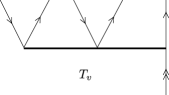
Figure 1: Diagrammatic representation of valence triple excitations. Double-headed arrow represents valence state.

To motivate more accurate, yet practical extension of the SD method, we consider numerical results for the reduced electric-dipole matrix elements of $3s_{1/2}-3p_{1/2}$ transition in Na Cannon and Derevianko (2004). From Table I of that paper, we observe that the contributions from valence triples $T_{v}$ (total $-4.4\times 10^{-3}$) and non-linear doubles (disconnected quadruples) $D_{nl}$ (total $1.3\times 10^{-3}$) are much larger than those from core triples $T_{c}$ (total $8\times 10^{-5}$). Similar conclusion can be drawn from our calculations for heavier Cs atom Derevianko and Porsev (2005). Because of this observation we will discard core triples and incorporate the valence triples into the SD formalism. We will refer to this method as SDvT approximation. Contributions of core triples to matrix elements are treated in this work perturbatively.

In addition to triples, we will include effects from disconnected excitations. The relevant diagrams contribute at the same level as the valence triples and the full treatment of disconnected excitations will recover a part of the otherwise missing sequence of random-phase-approximation diagrams (see also discussion in Ref. Derevianko and Porsev (2005)). The resulting approximation will be referred to as CCSDvT method.

III Formalism

Below we write down the CC equations for cluster amplitudes $\rho$ in the CCSDvT approximation. The equations in the SD approximation are presented in Ref. Blundell et al. (1989). We retain convention for the single and doubles from that paper and focus on additional terms due to valence triples and disconnected excitations. Some of the equations involving triple excitations were given in Ref. Safronova et al. (1998); Safronova et al. (1999a); we use a different convention for the triples amplitudes.

III.1 Valence triples

In the following, we employ fully antisymmetrized valence triples amplitude $\tilde{\rho}_{mnrvab}$. The object $\tilde{\rho}_{mnrvab}$ is antisymmetric with respect to any permutation of the indices $mnr$ or $ab$, e.g.,

$$\tilde{\rho}_{mnrvab}=-\tilde{\rho}_{nmrvab}=-\tilde{\rho}_{mnrvba}=\tilde{\rho}_{mrnvba}=\ldots\,.$$ (16)

It is straightforward to demonstrate that the contribution to the wave operator (and therefore all the resulting equations) can be expressed in terms of this antisymmetrized object. Explicitly,

$$T_{v}=\frac{1}{12}\sum_{mnrab}\tilde{\rho}_{mnrvab}\,a^{\dagger}_{m}a^{\dagger}_{n}a^{\dagger}_{r}a_{b}a_{a}a_{v}\,.$$ (17)

Computationally the use of $\tilde{\rho}_{mnrvab}$ substantially reduces storage requirements, as it is sufficient to store ordered amplitudes with $m>n>r$ and $a>b$ only. In the equations below, we will also use antisymmetrized combinations for doubles $\tilde{\rho}_{mnab}=\rho_{mnab}-\rho_{mnba}=\rho_{mnab}-\rho_{nmab}$, $\tilde{\rho}_{mnva}=\rho_{mnva}-\rho_{nmva}$, and for the Coulomb matrix elements $\tilde{g}_{ijkl}=g_{ijkl}-g_{ijlk}$.

From the general Eq.(9) we obtain symbolically

$$\left(\varepsilon_{a}+\varepsilon_{b}+\varepsilon_{v}-\varepsilon_{m}-\varepsilon_{n}-\varepsilon_{r}+\delta E_{v}\right)\tilde{\rho}_{mnrvab}=$$ (18)

$$T_{v}[D_{c}]+T_{v}[D_{v}]+T_{v}[T_{v}]+T_{v}[T_{c}]+\mathrm{nonlinear}\,.$$

Here contribution $T_{v}[D_{c}]$ denotes effect of core doubles on valence triples, the remaining terms defined in a similar fashion. In this work we include only contributions $T_{v}[D_{c}]$ and $T_{v}[D_{v}]$ (see Fig. 2) and omit the effect of valence and core triples on valence triples ( $T_{v}[T_{v}]$ and $T_{v}[T_{c}]$) and nonlinear CC contributions. Compared to the $T_{v}[D_{v}]$ and $T_{v}[D_{c}]$ contributions, these are higher order (and computationally expensive) effects. Explicitly,

$$T_{v}[D_{c}] = -\underset{c}{\sum}\left(\widetilde{g}_{mcva}\widetilde{\rho}_{nrcb}-\widetilde{g}_{mcvb}\widetilde{\rho}_{nrca}+\widetilde{g}_{ncva}\widetilde{\rho}_{rmcb}-\widetilde{g}_{ncvb}\widetilde{\rho}_{rmca}+\widetilde{g}_{rcva}\widetilde{\rho}_{mncb}-\widetilde{g}_{rcvb}\widetilde{\rho}_{mnca}\right)$$ (19)

$$+ \underset{s}{\sum}\left(\widetilde{g}_{nrsv}\widetilde{\rho}_{msab}+\widetilde{g}_{rmsv}\widetilde{\rho}_{nsab}+\widetilde{g}_{mnsv}\widetilde{\rho}_{rsab}\right)\,,$$

$$T_{v}[D_{v}] = \underset{c}{\sum}\left(\widetilde{g}_{mcab}\widetilde{\rho}_{nrvc}+\widetilde{g}_{ncab}\widetilde{\rho}_{rmvc}+\widetilde{g}_{rcab}\widetilde{\rho}_{mnvc}\right)$$ (20)

$$+ \underset{s}{\sum}\left(\widetilde{g}_{nrsb}\widetilde{\rho}_{msva}-\widetilde{g}_{nrsa}\widetilde{\rho}_{msvb}+\widetilde{g}_{rmsb}\widetilde{\rho}_{nsva}-\widetilde{g}_{rmsa}\widetilde{\rho}_{nsvb}+\widetilde{g}_{mnsb}\widetilde{\rho}_{rsva}-\widetilde{g}_{mnsa}\widetilde{\rho}_{rsvb}\right)\,.$$

Notice that the matching of diagrams in Eq.(9) is generally not unique; we require that the r.h.s. of the above equation is fully antisymmetrized as the amplitude $\tilde{\rho}_{mnrvab}$ on the l.h.s.; such procedure is unique and corresponds to a projecton of the CC equations onto the many-body state $a^{\dagger}_{m}a^{\dagger}_{n}a^{\dagger}_{r}a_{b}a_{a}|0_{c}\rangle$. Also from these equations we immediately observe that the triples enter the many-body wave function in the effective second order of MBPT, as the doubles enter in the first order in $G$, Eq.(13).

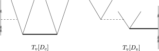
Figure 2: Representative contributions to the r.h.s of the valence triples equation. Horizontal dashed line denotes Coulomb interaction and solid lines — cluster amplitudes.

III.2 Modifications to SD equations and valence energies

Here we present CC equations for correlation energy $\delta E_{v}$, valence singles $\rho_{mv}$, and for valence double $\rho_{mnva}$ cluster amplitudes. In formulas below we write $\mathrm{SD}$ to denote contributions in the singles-doubles approximations tabulated in Refs. Blundell et al. (1989); Safronova et al. (1998). As to the core amplitudes, they will be determined in the SD approximation (i.e. we do not include non-linear CC terms and core triples).

Topological structure of the valence singles equation is

$$\left(\varepsilon_{v}-\varepsilon_{m}+\delta E_{v}\right)\rho_{mv}=\mathrm{SD}+$$ (21)

$$S_{v}[S_{c}\otimes S_{v}]+S_{v}[S_{c}\otimes S_{c}]+S_{v}[S_{c}\otimes D_{v}]+S_{v}[S_{v}\otimes D_{c}]+S_{v}[T_{v}]\,,$$

where notation $(K)_{n}\left[(K)_{p}\otimes(K)_{m}\right]$ stands for a contribution from a disconnected $(p+m)$–fold excitation (resulting from a product of clusters $(K)_{p}$ and $(K)_{m}$) to the cluster $(K)_{n}$. We do not include cubic non-linear term $S_{v}[S_{c}\otimes S_{c}\otimes S_{v}]$. Explicitly,

$$S_{v}[S_{c}\otimes S_{v}] = \underset{anr}{\sum}\tilde{g}_{amnr}\rho_{na}\rho_{rv}\,,$$ (22)

$$S_{v}[S_{c}\otimes S_{c}] = \underset{abn}{\sum}\tilde{g}_{abnv}\rho_{ma}\rho_{nb}\,,$$ (23)

$$S_{v}[S_{c}\otimes D_{v}] = \underset{abnr}{\sum}\tilde{g}_{abnr}\left(\rho_{mb}\rho_{nrva}-\rho_{nb}\tilde{\rho}_{mrva}\right)\,,$$ (24)

$$S_{v}[S_{v}\otimes D_{c}] = -\underset{abnr}{\sum}\tilde{g}_{abnr}\rho_{nv}\rho_{mrab}\,,$$ (25)

$$S_{v}[T_{v}] = \frac{1}{2}\underset{abnr}{\sum}g_{abnr}\tilde{\rho}_{mnrvab}\,.$$ (26)

Representative diagrams are shown in Fig. 3.

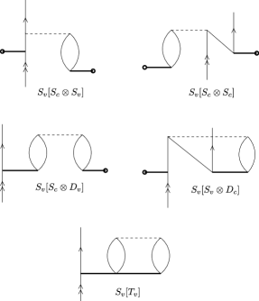
Figure 3: Sample contributions of triples and disconnected excitations to the valence singles equation.

Valence doubles equation for $\rho_{mnva}$ can be symbolically represented as (see Fig. 4)

$$\left(\varepsilon_{v}+\varepsilon_{a}-\varepsilon_{m}-\varepsilon_{n}+\delta E_{v}\right)\rho_{mnva}=\mathrm{SD}+$$

$$D_{v}[S_{c}\otimes S_{v}]+D_{v}[S_{c}\otimes S_{c}]+$$

$$D_{v}[S_{c}\otimes D_{v}]+D_{v}[S_{v}\otimes D_{c}]+D_{v}[S_{c}\otimes D_{c}]+$$

$$D_{v}[D_{c}\otimes D_{v}]+D_{v}[S_{c}\otimes T_{v}]+D_{v}[S_{v}\otimes T_{c}]+D_{v}[T_{v}]\,.$$

Contribution $D_{v}[D_{c}\otimes D_{c}]$ is topologically impossible and we omit cubic and higher-degree nonlinear terms like $D_{v}[S_{c}\otimes S_{c}\otimes S_{v}]$, $D_{v}[S_{c}\otimes S_{c}\otimes D_{v}]$, and $D_{v}[S_{v}\otimes S_{c}\otimes S_{c}\otimes S_{c}]$.

Explicitly,

$$D_{v}[D_{c}\otimes D_{v}] =\underset{bcrs}{\sum}g_{bcrs}\left\{\rho_{rsva}\rho_{mnbc}+\frac{1}{2}\tilde{\rho}_{msva}\rho_{nrbc}\right.$$

$$\left.+\frac{1}{2}\tilde{\rho}_{snva}\rho_{mrbc}+\tilde{\rho}_{rsvb}\rho_{nmac}+\tilde{\rho}_{rsab}\rho_{mnvc}\right\}\,$$

$$-\underset{bcrs}{\sum}\tilde{g}_{bcrs}\tilde{\rho}_{msvb}\tilde{\rho}_{nrac},$$

$$D_{v}[S_{v}\otimes D_{c}] =-\sum_{brs}\tilde{g}_{bmrs}\,\rho_{rv}\,\tilde{\rho}_{nsab}+\sum_{bcr}g_{bcar}\,\rho_{rv}\,\rho_{nmbc}\,,$$

$$D_{v}[S_{c}\otimes D_{v}] =\frac{1}{2}\sum_{brs}\tilde{g}_{bnrs}\,\rho_{rb}\,\tilde{\rho}_{msva}\,\,\,-\frac{1}{2}\sum_{brs}\tilde{g}_{bmrs}\,\rho_{rb}\,\tilde{\rho}_{nsva}\,\,$$

$$+\frac{1}{2}\sum_{brs}g_{bmrs}\,\rho_{nb}\,\tilde{\rho}_{rsva}\,\,-\frac{1}{2}\sum_{brs}g_{bnrs}\,\rho_{mb}\,\tilde{\rho}_{rsva}$$

$$-\sum_{brs}\tilde{g}_{bnrs}\,\rho_{ra}\,\tilde{\rho}_{msvb}-\sum_{bcr}\tilde{g}_{bcar}\,\rho_{rc}\,\rho_{mnvb}-\sum_{bcr}\tilde{g}_{bcar}\,\rho_{nc}\,\tilde{\rho}_{rmvb}\,,$$

$$D_{v}[S_{c}\otimes D_{c}] =-\sum_{bcr}\tilde{g}_{bcvr}\,\rho_{rc}\,\rho_{nmab}\,-\sum_{bcr}\tilde{g}_{bcvr}\,\rho_{mc}\,\tilde{\rho}_{rnab}\,+\,\sum_{bcr}g_{bcvr}\,\rho_{ra}\,\rho_{mnbc}\,,$$

$$D_{v}[S_{c}\otimes S_{v}] =\sum_{br}\tilde{g}_{bnar}\,\rho_{mb}\,\rho_{rv}\,\,+\sum_{rs}g_{mnrs}\,\rho_{rv}\,\rho_{sa}\,,$$

$$D_{v}[S_{c}\otimes S_{c}] =\sum_{br}\tilde{g}_{bmvr}\,\rho_{nb}\,\rho_{ra}+\sum_{bc}g_{bcav}\,\rho_{mc}\,\rho_{nb}\,.$$

The effect of valence triples on valence doubles reads

$$D_{v}[T_{v}] = -\frac{1}{2}\underset{rbc}{\sum}\left(g_{bcar}\tilde{\rho}_{mnrvbc}+g_{bcvr}\tilde{\rho}_{nmrabc}\right)$$

$$+ \frac{1}{2}\underset{rsb}{\sum}\left(g_{bnrs}\tilde{\rho}_{msrvab}+g_{bmrs}\tilde{\rho}_{snrvab}\right)\,.$$

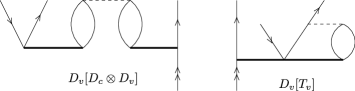
Figure 4: Effects of disconnected and valence triple excitations on valence doubles.

Finally, the valence correlation energy may be represent as

$$\delta E_{v}=\delta E_{\mathrm{SD}}+\delta E_{\mathrm{CC}}+\delta E_{\mathrm{vT}}\,,$$ (28)

with

$$\delta E_{\mathrm{CC}} = \underset{anr}{\sum}\ \tilde{g}_{avnr}\rho_{na}\rho_{rv}+\underset{abn}{\sum}\ \tilde{g}_{abnv}\rho_{va}\rho_{nb}$$

$$+ \underset{abnr}{\sum}\ \tilde{g}_{abnr}\left[\rho_{vb}\rho_{nrva}-\rho_{nb}\tilde{\rho}_{vrva}-\rho_{nv}\rho_{vrab}\right]\,,$$

$$\delta E_{\mathrm{vT}} = \frac{1}{2}\underset{abmn}{\sum}\ g_{abmn}\tilde{\rho}_{vmnvab}\,.$$ (30)

Topological structure of contributions to energy is similar to the terms on the r.h.s of the valence singles equation (21). Here correction $\delta E_{\mathrm{CC}}$ comes from non-linear CC contributions and $\delta E_{\mathrm{vT}}$ is due to valence triples.

III.3 Normalization

The CC wave function is derived using the intermediate normalization, $\langle\Psi_{v}^{(0)}|\Psi_{v}\rangle=1$ and in calculating the atomic properties based on the CC wave function, one needs to renormalize it. In calculations of matrix elements one requires the valence part of the normalization, $N_{v}=\langle\Psi_{v}|\Psi_{v}\rangle_{\mathrm{val,connected}}$. We obtain

$$N_{v}=\mathrm{SD}+\underset{mnab}{\sum}\rho_{mnab}\,\tilde{\rho}_{vmnvab}+\frac{1}{12}\underset{mnrab}{\sum}(\tilde{\rho}_{mnrvab})^{2}\,.$$ (31)

The last term in the equation above is quadratic in valence triples (i.e., it is of the fourth effective order) and we will neglect it in the following.

III.4 Matrix elements of one-body operator

Finally, we consider matrix elements of a one-body operator $Z=\sum_{ij}z_{ij}a_{i}^{\dagger}a_{j}$ between two CC states $|\Psi_{v}\rangle$ and $|\Psi_{w}\rangle$. Taking into account renormalization, this matrix element can be defined as

$$\mathcal{M}_{wv}\equiv\frac{\langle\Psi_{w}|Z|\Psi_{v}\rangle}{\sqrt{N_{w}N_{v}}}$$ (32)

As it was shown in Ref. Blundell et al. (1989) all disconnected diagrams in the numerator and denominator of this expression cancel, leading to

$$\mathcal{M}_{wv}=\frac{\left(Z_{wv}^{\mathrm{val}}\right)_{\mathrm{conn}}}{\left\{\left[1+\left(N_{v}^{\mathrm{val}}\right)_{\mathrm{conn}}\right]\left[1+\left(N_{w}^{\mathrm{val}}\right)_{\mathrm{conn}}\right]\right\}^{1/2}}\,.$$ (33)

We discarded valence-independent contribution, as it vanishes for non-scalar operators. To unclutter the notation below we simply write

$$Z_{wv} \equiv (Z_{wv}^{\mathrm{val}})_{\mathrm{conn}},$$

$$N_{v} \equiv (N_{v}^{\mathrm{val}})_{\mathrm{conn}}\,.$$ (34)

Blundell et al. (1989) tabulated 21 contributions to the matrix elements in the SD approximation. These SD corrections are mainly due to (i) random-phase-approximation (RPA) diagram proportional to a product of $Z$ and $D_{v}$ and (ii) the Brueckner-type (core-polarization) diagram proportional to the product of $Z$ and $S_{v}$. In Ref. Derevianko and Porsev (2005) we additionally included modifications to $\mathcal{M}_{wv}$ caused by non-linear terms in the CC wave function. We have devised a re-summation scheme that is equivalent to “dressing” of lines and vertices of the SD diagrams (see also Ref. Martensson-Pendrill and Ynnerman (1990)).

Including valence triples leads to additional direct contributions, $Z_{wv}={\rm SD}+Z_{wv}^{\left(T_{v}\right)}$. We obtain

$$Z_{wv}^{\left(T_{v}\right)} = \sum_{k=1}^{7}Z_{wv}^{\left(T_{v},k\right)}\,,$$ (35)

$$Z_{wv}^{\left(T_{v},1\right)} = \underset{abmn}{\sum}\rho_{ma}^{*}\tilde{\rho}_{wmnvab}z_{bn}+{\rm h.c.s.},$$ (36)

$$Z_{wv}^{\left(T_{v},2\right)} = -\frac{1}{2}\underset{abcmn}{\sum}\tilde{\rho}_{mnba}^{*}\tilde{\rho}_{wnmvcb}z_{ca}+{\rm h.c.s.},$$ (37)

$$Z_{wv}^{\left(T_{v},3\right)} = \frac{1}{4}\underset{abmnr}{\sum}\tilde{\rho}_{mnab}^{*}\tilde{\rho}_{rmnvab}z_{wr}+{\rm h.c.s.},$$ (38)

$$Z_{wv}^{\left(T_{v},4\right)} = \frac{1}{2}\underset{abmnr}{\sum}\tilde{\rho}_{mnab}^{*}\tilde{\rho}_{wrmvba}z_{nr}+{\rm h.c.s.},$$ (39)

$$Z_{wv}^{\left(T_{v},5\right)} = -\frac{1}{2}\underset{abmnr}{\sum}\tilde{\rho}_{mnwb}^{*}\tilde{\rho}_{rmnvab}z_{ar}+{\rm h.c.s.},$$ (40)

$$Z_{wv}^{\left(T_{v},6\right)} = -\frac{1}{6}\underset{abcmnr}{\sum}\tilde{\rho}_{mnrwcb}^{\ast}\tilde{\rho}_{mnrvab}z_{ac},$$ (41)

$$Z_{wv}^{\left(T_{v},7\right)} = \frac{1}{4}\underset{abmnrs}{\sum}\tilde{\rho}_{mnrwab}^{\ast}\tilde{\rho}_{snrvab}z_{ms}\,.$$ (42)

In these expressions, abbreviation h.c.s. stands for a Hermitian conjugation of the preceding term with a simultaneous swap of the valence indices $w\leftrightarrow v$. As discussed in Ref. Derevianko and Emmons (2002), valence triples start contributing in the fourth order of MBPT for matrix elements; these contributions correspond to terms $Z_{wv}^{\left(Tv,k\right)},k=2-5$. We presently discard terms #6 and #7 that are quadratic in triple excitations.

III.5 Symmetries and reduced triples

Relativistic one-particle orbitals $i$ are characterized by the principle quantum number $n_{i}$, the total angular momentum $j_{i}$, it’s projection $m_{i}$ and the orbital angular momentum $l_{i}$. The summations over magnetic quantum numbers are carried out analytically, substantially reducing the number of coefficients. A dependence of valence triples on magnetic quantum numbers may be parameterized as (we use angular diagrams, see, e.g., Ref. Lindgren and Morrison (1986))

$$\tilde{\rho}_{mnrvab}=\sum_{LL^{\prime}h}\raisebox{-25.83325pt}{\includegraphics[scale={0.6}]{angdia_triples.eps}}\tilde{F}_{LL^{\prime}h}\left(mnr\,vab\right)\,,$$ (43)

where $h$ is a half-integer coupling angular momentum and $L$ and $L^{\prime}$ are integer coupling momenta. The “reduced triples” $\tilde{F}_{LL^{\prime}~{}h}\left(mnrvab\right)$ do not depend on magnetic quantum numbers.

Selection rules for various angular momenta characterizing reduced triples follow from properties of the $3j$-symbols in the angular diagram (43). In addition, the atomic Hamiltonian is invariant under parity transformation, leading to an additional parity selection rule $l_{m}+l_{n}+l_{r}+l_{v}+l_{a}+l_{b}=\mathrm{even\,integer}$ for a triple amplitude $\tilde{\rho}_{mnrvab}$.

Owing to the antisymmetric properties of the triples, Eq.(16), it is sufficient to store reduced triples with $(n_{m}\varkappa_{m})\geq(n_{n}\varkappa_{n})\geq(n_{r}\varkappa_{r})$ and $(n_{a}\varkappa_{a})\geq(n_{b}\varkappa_{b})$, where $\varkappa=(l-j)(2j+1)$. The reduced triples with other combinations of arguments can be related to the ordered set via symmetry properties. For example,

$$\tilde{F}_{LL^{\prime}h}\left(mnr\,vba\right)=(2h+1)\,(2L^{\prime}+1)\,\sum_{h^{\prime}K}\left\{\begin{array}[c]{ccc}j_{b}&h&L\\ j_{r}&L^{\prime}&j_{a}\\ K&j_{n}&h^{\prime}\end{array}\right\}\,{\left(-1\right)}^{h+h^{\prime}+K+L^{\prime}}\,{\tilde{F}}_{LKh^{\prime}}(mnr\,vab)\,\,.$$ (44)

There are 11 such index-swapping relations for reduced valence triples.

IV Numerical results and discussion

To reiterate discussion so far, we derived algebraic expressions in the CCSDvT formalism, which includes valence triples and a subset of disconnected excitations. We also carried out angular reduction of these expressions and developed a numerical code. In this section we present our ab initio results for properties of $3s$, $3p_{1/2}$, and $3p_{3/2}$ states of atomic sodium. Results for removal energies are presented in Section IV.1 and for dipole matrix elements and HFS constants $A$ in Section IV.2.

Before presenting the results, let us briefly describe our numerical code. It is an extension of the relativistic SD code Safronova et al. (1998) which employs B-spline basis set. This basis numerically approximates complete set of single-particle atomic states. Here we use 35 out of 40 positive-energy ($\varepsilon_{i}>-m_{e}c^{2}$) basis functions. Basis functions with $l_{\rm max}\leq 6$ are used for singles and doubles. For triples we employ a more limited set of basis functions with $l_{\rm max}(T_{v})\leq 4$. Excitations from all core sub-shells are included in the calculations. Numerically we found that this choice is a reasonable trade-off between storage and overall numerical accuracy (after all, triples affect computed properties at $\sim 1$% level.) The results presented in this Section will include basis set extrapolation correction, which is obtained by computing SD properties with increasingly larger basis sets and interpolating them to $l=\infty$. The CC equations were solved iteratively. We notice that the reported calculations can be carried out in the memory of a modern high-end personal workstation: storing reduced valence triples in a single precision required about 900 Mb for $s_{1/2}$ states and 1.5 Gb for $p_{3/2}$ states (the latter involve more angular channels).

IV.1 Energies

Computed removal energies of $3s$, $3p_{1/2}$, and $3p_{3/2}$ states of atomic sodium are presented in Table 1. The dominant contribution to the energies comes from the DHF values. The remaining (correlation) contribution is given by Eq. (28). We computed this correlation correction in several approximations: SD, SDvT, CCSD, and, finally, CCSDvT.

Table 1: Contributions to removal energies of $3s$, $3p_{1/2}$, and $3p_{3/2}$ states for Na in cm^-1 in various approximations. A comparison with previous CC-type calculations and experimental values is presented in the lower panel.

	$3s$	$3p_{1/2}$	$3p_{3/2}$
$E_{\rm DHF}$	$39951.6$	$24030.4$	$24014.1$
SD
$\delta E_{\rm SD}$	$1488.8$	$463.9$	$460.6$
$E^{\rm tot}_{\rm SD}$	$41440.3$	$24494.3$	$24474.7$
SDvT
$\delta E_{\rm SD}^{\rm indir}$	$79.7$	$28.9$	$28.4$
$\delta E_{\rm vT}$	$25.4$	$4.8$	$4.7$
$E^{\rm tot}_{\rm SDvT}$	$41545.5$	$24528.0$	$24507.8$
CCSD
$\delta E_{\rm SD}^{\rm indir}$	$-57.0$	$-20.0$	$-18.4$
$\delta E_{\rm CC}$	$-17.5$	$-7.4$	$-7.4$
$E^{\rm tot}_{\rm CCSD}$	$41365.9$	$24466.9$	$24448.9$
CCSDvT
$\delta E_{\rm SD}^{\rm indir}$	$16.8$	$6.8$	$7.9$
$\delta E_{\rm vT}$	$23.7$	$4.5$	$4.4$
$\delta E_{\rm CC}$	$-18.4$	$-8.0$	$-8.0$
$E^{\rm tot}_{\rm CCSDvT}$	$41462.5$	$24497.6$	$24479.1$
Other works
SD(pvT)  Safronova et al. (1999a)	$41447.3$	$24493.9$	$24476.7$
CCSD Eliav et al. (1994)	$41352$	$24465$
$E_{\rm experim}$	$41449.6$	$24493.4$	$24476.2$

These values are from spectroscopic data compiled by NIST NIS

First we list correlation energies $\delta E_{\rm SD}$ obtained in the SD approximation. The results contain basis set extrapolation corrections from Ref. Safronova (2000). The extrapolation corrections increase the removal energies by 5.1 cm^-1 for the $3s$ state, 1.9 cm^-1 for the $3p_{1/2}$ state, and 0.8 cm^-1 for the $3p_{3/2}$. Total removal energy is $E^{\mathrm{tot}}_{\mathrm{SD}}=E_{\mathrm{DHF}}+\delta E_{\mathrm{SD}}$. At the next step (SDvT) we include valence triple excitations, i.e., in the CC equations in addition to the SD terms we incorporate terms with amplitudes $\tilde{\rho}_{mnrvab}$. It is instructive to distinguish direct and indirect $\delta E_{\rm SD}^{\rm indir}$ effects of these excitations. The direct effect of triples is $\delta E_{\mathrm{vT}}$, Eq.(30), while indirect effect is a modification of $\delta E_{\mathrm{SD}}$ due to effect of triples through coupling to singles and doubles. In this case, the indirect contribution is defined as $\delta E_{\rm SD}^{\rm indir}=\delta E_{\rm SD}[{\rm SDvT}]-\delta E_{\rm SD}[{\rm SD}]$. We list the two types of contributions in the Table and it is clear that for all the states both contributions add constructively, and for all the considered approximations the indirect contribution dominates over the direct one. The total removal energy in the SDvT approximation is $E^{\mathrm{tot}}_{\mathrm{SDvT}}=E_{\mathrm{DHF}}+\delta E_{\mathrm{SD}}+\delta E_{\rm SD}^{\rm indir}+\delta E_{\mathrm{vT}}$. The totals for other approximations are defined in a similar way.

As we move to the CCSD approximation in Table 1, we notice that here the corrective terms $\delta E_{\rm SD}^{\rm indir}$ and $\delta E_{\rm CC}$ decrease the removal energies, while for the SDvT case the corrections increased $E^{\mathrm{tot}}$. In both cases the resulting total energies $E^{\mathrm{tot}}$ were moved away from the experimental values. Since the effects of disconnected and triple excitations are comparable and opposite in sign, simultaneous treatment of the two effects is required. The results of such treatment are listed under CCSDvT heading in the Table. Compared to the CCSD and SDvT approximations, the CCSDvT results move into a closer, 0.01-0.03%, agreement with the experimental values.

Comparison with the previous CC-type calculations of Na removal energies is presented in the lower panel of the Table 1. SD(pvT) approximation denotes results obtained with a scheme originally proposed in Ref. Blundell et al. (1991). In this scheme: (i) starting from the SDvT approximation, one keeps vT contributions in the equation for valence singles and valence energies (i.e., $D_{v}[T_{v}]$ effect is neglected) ; (ii) triples are approximated by

$$\tilde{\rho}_{mnrvab}\approx\frac{T_{v}[D_{c}]+T_{v}[D_{v}]}{\varepsilon_{a}+\varepsilon_{b}+\varepsilon_{v}-\varepsilon_{m}-\varepsilon_{n}-\varepsilon_{r}+\delta E_{v}};$$

(iii) to avoid expensive storing of valence triples, in the $\rho_{mv}$ equation the triples denominators $\left({\varepsilon_{a}+\varepsilon_{b}+\varepsilon_{v}-\varepsilon_{m}-\varepsilon_{n}-\varepsilon_{r}+\delta E_{v}}\right)$ are replaced by an approximate combination $\left({\varepsilon_{a}+\varepsilon_{b}-\varepsilon_{n}-\varepsilon_{r}}\right)$. In this approximation $S_{v}[T_{v}]$ effect is effectively overemphasized ( for the ground state $\varepsilon_{v}<\varepsilon_{m}$ ). In the expression for the energy, $\delta E_{\mathrm{vT}}$, Eq.(30), triples enter as $\tilde{\rho}_{vmnvab}$ and the above replacement of denominators is more algebraically justified. Nevertheless, we found a substantial (a factor of three) disagreement between $\delta E_{\mathrm{vT}}$ corrections obtained in our (more complete) SDvT and SD(pvT) approximations.

To understand the origin of this large disagreement, we have compared individual contributions to $\delta E_{\mathrm{vT}}$ coming from the r.h.s. of the triples equations with the corresponding contributions in the SD(pvT) approximation. We found that the individual terms agree at a reasonable 10% level. The discrepancy in the total value arises because there are certain very large individual terms canceling each other. These terms are several hundred times larger then the final combined result. In other words there is a subtle cancelation taking place and our more sophisticated all-order treatment profoundly affects this delicate cancelation.

In addition, in Ref. Safronova et al. (1998), the explicit contributions of triples to the energies, $\delta E_{\mathrm{vT}}$, were computed using direct third-order MBPT approach. Such terms are denoted in Ref. Safronova et al. (1998) as $E^{(3)}_{v,{\rm extra}}$, to emphasize that these are diagrams missed in the SD approximation in the third order. A comparison of our computed $\delta E_{\mathrm{vT}}$ with $E^{(3)}_{v,{\rm extra}}$ is presented in Table 2. We again observe a large discrepancy, due to substantial cancelations among contributions to $E^{(3)}_{v,{\rm extra}}$ and resulting enhanced sensitivity to a correct all-order treatment.

The CCSD results obtained by Eliav et al. (1994) agrees with our CCSD energies for the $3p_{1/2}$ state. However, for the $3s_{1/2}$ the two calculations disagree by 14 cm^-1. This discrepancy is likely due to our omission of all non-linear terms in the core CCSD equations.

Table 2: Comparison of complementary third-order MBPT contributions $E^{(3)}_{v,\,{\rm extra}}$ to removal energies with the corresponding all-order correction $\delta E_{\mathrm{vT}}$. The corrections are given in cm^-1.

	$3s$	$3p_{1/2}$	$3p_{3/2}$
$\delta E_{\mathrm{vT}}$	$-25.4$	$-4.8$	$-4.7$
$E^{(3)}_{v\,,{\rm extra}}$, Ref. Safronova et al. (1998)	$-9.2$	$-1.5$	$-1.6$

Comparing the final CCSDvT results for the removal energies with the experimental values (last row of Table 2) we find an agreement at the level of 0.01-0.03%. We do not include Breit-, reduced-mass and mass-polarization corrections to the energies, as they contribute at a much smaller level Safronova et al. (1998). A perfect theory-experiment agreement for the previous SD(pvT) calculations of energies Safronova et al. (1999a) is fortuitous because contributions of the disconnected excitations omitted in Ref. Safronova et al. (1999b) would move the theoretical energies by about 70 cm^-1 for the $3s_{1/2}$ state (see Table 1).

IV.2 Hyperfine constants and electric-dipole amplitudes

With the computed wave functions of the $3s$, $3p_{1/2}$ and $3p_{3/2}$ states we proceed to determining magnetic-dipole hyperfine-structure constants $A$ and electric-dipole transition amplitudes. The formalism was outlined in Sec. III.4 and here we discuss our ab initio results and compare them with the experimental values.

Numerical results are presented in Table 3. This Table is organized as follows. First we list the DHF and SD values. The results for the HFS constants include finite-nuclear size effects (see Appendix). In the part denoted “All-order corrections beyond SD” we tabulate differences between the values obtained at a certain approximation (CCSD, SDvT, CCSDvT) and the corresponding SD value (symbolically, e.g., $\Delta(\mathrm{CCSD})=\mathrm{CCSD}-\mathrm{SD}$). The most sophisticated approximation is CCSDvT (it includes both implicit and explicit, Eq. (35), contributions of valence triples and implicit contribution of disconnected excitations); we will base our final ab initio result on the CCSDvT values. A cursory look at this part of the Table reveals that the contributions of disconnected excitations tend to compensate contributions of valence triples for all the computed properties. This situation is similar to the one observed by us while presenting results for removal energies in Section IV.1.

While discussing the CCSDvT results, it is instructive to compare the explicit valence triple corrections to matrix elements, Eq.(35), with a corresponding contribution from the direct fourth-order calculations Cannon and Derevianko (2004). In particular, for the $\langle 3s||D||3p_{1/2}\rangle$ amplitude, the $Z_{wv}^{\left(T_{v}\right)}$ CCSDvT contribution of -0.00075 is in a close agreement with the fourth-order $Z_{1\times 2}(T_{v})$ contribution of -0.00073. The close agrement is due to the fact that there are no strongly canceling terms in the $Z_{1\times 2}(T_{v})$ class of the fourth-order diagrams. This should be contrasted with our similar comparison of energy corrections (see Table 2), where large, a factor of 100, cancelations lead to a poor accuracy of the direct third-order computation.

Corrections beyond the CCSDvT approximation are listed in the Table 3 under the heading “Complementary corrections”. The dressing corrections arise due to a direct contribution of disconnected excitations to the matrix elements. The details of our all-order dressing scheme can be found in Ref.Derevianko and Porsev (2005). Following that work we distinguish between vertex- and line- dressing corrections. Futher, the “MBPT-IV” entries in the Table include all IVth diagrams missed by the CCSDvT method and dressing. For example, our CCSDvT approximation discards core triples and disconnected core excitations and these contributions arise starting from the fourth order of MBPT for matrix elements. In notation of Ref. Derevianko and Emmons (2002) the complementary fourth-order terms are $Z_{0\times 3}(D_{v}[T_{c}])$, $Z_{0\times 3}(S_{c}[T_{c}])$, and $Z_{1\times 2}(T_{c})$. In addition, the dressing method of Ref.Derevianko and Porsev (2005) misses so-called stretched and ladder $Z_{1\times 2}(D_{nl})$ diagrams. These diagrams are also incorporated into the value of “MBPT-IV” contribution in the Table 3. We used the fourth-order code of Ref. Cannon and Derevianko (2004) to evaluate the complementary MBPT-IV contributions.

Finally, we tabulate Breit and QED corrections available from the literature (see Appendix for discussion). By combining them with the CCSDvT values and the complementary corrections we arrive at the final ab initio values in the bottom part of Table 3. Here we also present a comparison with the experimental data. In particular, the last row tabulates percentage deviations from the experimental values. If the ab initio value lays inside the experimental error bar, we tabulate experimental uncertainty instead. The theory-experiment agreement is better than 0.1% except for the HFS constant of the $3p_{3/2}$ state, where our value disagrees with most accurate experimental results at 1% level. For this constant our result is, however, in a reasonable agreement with the less accurate (0.3% uncertainty) result of Ref. Krist et al. (1977).

Table 3: Hyperfine structure constants $A$ (in MHz) and matrix elements of electric dipole moment (in a.u.) for ²³Na. Results of calculations and comparison with experimental values. See text for the explanation of entries.

	$A(3s)$	$A(3p_{1/2})$	$A(3p_{3/2}$)	$\langle 3p_{1/2}||D||3s\rangle$	$\langle 3p_{3/2}||D||3s\rangle$
DHF	$623.8$	$63.39$	$12.59$	$3.6906$	$5.2188$
SD	$889.0$	$95.05$	$18.85$	$3.5308$	$4.9932$
All-order corrections beyond SD
$\Delta$(CCSD)	$-7.7$	$-1.76$	$-0.34$	$0.0072$	$0.0098$
$\Delta$(SDvT)	$8.6$	$2.06$	$0.36$	$-0.0115$	$-0.0166$
$\Delta$(CCSDvT)	$0.4$	$0.07$	$-0.02$	$-0.0035$	$-0.0053$
Complementary corrections
Line dressing	$-2.4$	$-0.43$	$-0.09$	$0.0004$	$0.0005$
Vertex dressing	$1.5$	$0.17$	$0.04$	$-0.0001$	$-0.0002$
MBPT-IV (core triples,…)	$-2.8$	$-0.41$	$-0.06$	$0.0001$	$0.0001$
Breit + QED Sapirstein and Cheng (2003, 2005)	$0.2$			$0.0001$	$0.0002$
Final CCSDvT + corrections	$885.9$	$94.45$	$18.72$	$3.5278$	$4.9885$
Experiment	$885.81$	$94.44(13)$	$18.534(15)$	$3.5267(17)$	$4.9875(24)$
		$94.42(19)$	$18.572(24)$	$3.5246(23)$	$4.9839(34)$
			$18.64(6)$
			$18.69(9)$
Agreement with experiment	$0.01\%$	$<0.1\%$	$1\%$	$<0.05\%$	$<0.05\%$

Ref. Beckman et al. (1974); Ref. Wijngaarden and Li (1994); Ref. Yei et al. (1993); Ref. Jones et al. (1996); Ref. Carlsson et al. (1992); Ref. Gangrsky et al. (1998); Ref. Volz and Schmoranzer (1996); Ref. Krist et al. (1977); Ref. Arimondo et al. (1977).

V Conclusion

To reiterate here we presented a practical high-accuracy ab initio relativistic technique for calculating properties of univalent atomic systems. The distinct formal improvements over the previous singles-doubles approach Blundell et al. (1989, 1991); Safronova et al. (1998); Safronova et al. (1999a) are:

1. non-perturbative treatment of valence triple excitations;

2. incorporation of disconnected excitations (non-linear terms) in the coupled-cluster approach;

3. inclusion of complementary MBPT diagrams so that the calculations of matrix elements are complete through the fourth-order of MBPT; these diagrams include contributions of core triples.

4. all-order “dressing” of lines and vertices in calculations of matrix elements.

Including all the enumerated effects is important in reaching the present uniform “better than 0.1%” theoretical accuracy for Na atom. In particular, a simultaneous treatment of triple and disconnected quadruple excitations is required, as these two relatively large effects tend to partially cancel each other.

In the framework of the developed formalism, we computed removal energies, magnetic-dipole HFS constants $A$ and electric-dipole amplitudes for the principal $3s_{1/2}-3p_{j}$ transitions. The presented approach demonstrates a uniform sub-0.1%-accurate agreement with experimental data. In particular, we find that the removal energies are reproduced within 0.01-0.03% and the HFS constants of the $3s$ and $3p_{1/2}$ states with a better than 0.1% accuracy. The calculated dipole amplitudes are in a perfect agreement with the 0.05%-accurate experimental data. In the case of the $3p_{3/2}$ state HFS constant our ab initio result deviates from $\sim$ 0.1%-accurate experimental values Yei et al. (1993); Gangrsky et al. (1998) by 1%, while agreeing with the less accurate measurements Krist et al. (1977); Arimondo et al. (1977). We anticipate that the relativistic many-body technique presented here can serve as a basis of highly-accurate evaluation of parity-violating effects in Cs atom and Ba⁺ ion Koerber et al. (2003).

Appendix A Smaller (non-correlation) corrections to the hyperfine structure constants

Calculations of magnetic hyperfine constants $A$ presented in Table 3 were carried out with the nuclear gyromagnetic ratio $g_{I}=1.4784$. In calculations we model the nucleus as a uniformly magnetized sphere of radius 3.83 fm. For the $3s_{1/2}$ state, the corresponding nuclear size (Breit-Weisskopf) effect reduces point-nucleus results by 0.5 MHz. In an extreme case, when magnetization is assumed to be completely localized on the nuclear surface, the $A_{\mathrm{hfs}}(3s_{1/2})$ is further reduced by 0.15 MHz; this difference between the uniform and surface magnetization is below our theoretical accuracy.

Breit and QED contributions to the HFS constant of the $3s_{1/2}$ state were calculated recently by Sapirstein and Cheng (2003). In their notation, the value marked “Breit/QED” includes effects of the Breit interaction, retardation in the transverse photon exchange and negative-energy states, while “QED” correction encapsulates vacuum polarization and self-energy corrections. (The Breit correction of 0.35 MHz, evaluated using analytical expression Sushkov (2001) is in a reasonable agreement with the value of 0.2 MHz from Sapirstein and Cheng (2003)). As to the QED corrections, the leading Schwinger term (anomalous magnetic moment) $\delta A/A=\alpha/\pi$ sets a scale for radiative corrections at 0.1% and this is comparable with the accuracy of our calculations. Nevertheless, explicit model-potential calculation Sapirstein and Cheng (2003) of vacuum polarization and self-energy corrections displays a large degree of cancelation between different contributions, leading to the total QED correction 70 times smaller than the Schwinger term.

Following discussion of Ref. Yan et al. (1996) for Li, we also analyzed the following smaller corrections to the HFS constant: (i) Mass scaling. This effect contributes at the relative level of $1/(1+m_{e}/M_{\rm nuc})^{3}\approx 7\times 10^{-3}$ %; here $M_{\rm nuc}$ is the nuclear mass. (ii) Mass polarization. It occurs due to an additional introduction of the term $-\mu/M_{\mathrm{nuc}}\sum_{i>j}\mathbf{\nabla}_{i}\cdot\mathbf{\nabla}_{j}$ into the atomic Hamiltonian, $\mu$ being the reduced mass of the electron. We expect that this term would contribute at the relative level of $1/M_{\mathrm{nuc}}(\alpha Z)^{2}\approx 10^{-5}$ %. (iii) Second order in magnetic-dipole HFS interaction. It contributes at the $10^{-5}$ % level. All the enumerated corrections are below the level of theoretical accuracy of the calculation presented here.

References

- Khriplovich (1991) I. B. Khriplovich, Parity Nonconservation in Atomic Phenomena (Gordon & Breach, Philadelphia, 1991).
- Bouchiat and Bouchiat (1997) M.-A. Bouchiat and C. Bouchiat, Rep. Prog. Phys. 60, 1351 (1997).
- Wood et al. (1997) C. S. Wood, S. C. Bennett, D. Cho, B. P. Masterson, J. L. Roberts, C. E. Tanner, and C. E. Wieman, Science 275, 1759 (1997).
- Koerber et al. (2003) T. W. Koerber, M. H. Schacht, W. Nagourney, and E. N. Fortson, J. Phys. B 36, 637 (2003).
- Sapirstein and Cheng (2003) J. Sapirstein and K. T. Cheng, Phys. Rev. A 67, 022512 (2003).
- Coester and Kümmel (1960) F. Coester and H. G. Kümmel, Nucl. Phys. 17, 477 (1960).
- Čìžek (1966) J. Čìžek, J. Chem. Phys. 45, 4256 (1966).
- Blundell et al. (1989) S. A. Blundell, W. R. Johnson, Z. W. Liu, and J. Sapirstein, Phys. Rev. A 40, 2233 (1989).
- Blundell et al. (1991) S. A. Blundell, W. R. Johnson, and J. Sapirstein, Phys. Rev. A 43, 3407 (1991).
- Eliav et al. (1994) E. Eliav, U. Kaldor, and Y. Ishikawa, Phys. Rev. A 50, 1121 (1994).
- Avgoustoglou and Beck (1998) E. N. Avgoustoglou and D. R. Beck, Phys. Rev. A 57, 4286 (1998).
- Safronova et al. (1998) M. S. Safronova, A. Derevianko, and W. R. Johnson, Phys. Rev. A 58, 1016 (1998).
- Safronova et al. (1999a) M. S. Safronova, W. R. Johnson, and A. Derevianko, Phys. Rev. A 60, 4476 (1999a).
- Gopakumar et al. (2001) G. Gopakumar, H. Merlitz, S. Majumder, R. K. Chaudhuri, B. P. Das, U. S. Mahapatra, and D. Mukherjee, Phys. Rev. A. 64, 032502 (2001).
- Chaudhuri et al. (2003) R. K. Chaudhuri, B. K. Sahoo, B. P. Das, H. Merlitz, U. S. Mahapatra, and D. Mukherjee, J. Chem. Phys. 119, 10633 (2003).
- Salomonson and Ynnerman (1991) S. Salomonson and A. Ynnerman, Phys. Rev. A 43, 88 (1991).
- Derevianko and Porsev (2005) A. Derevianko and S. G. Porsev, Phys. Rev. A 71, 032509 (2005).
- Yei et al. (1993) W. Yei, A. Sieradzan, and M. D. Havey, Phys. Rev. A 48, 1909 (1993).
- Gangrsky et al. (1998) Yu. P. Gangrsky, D. V. Karaivanov, K. P. Marinova, B. N. Markov, L. M. Melnikova, G. V. Mishinsky, S. G. Zemlyanoi, and V. I. Zhemenik, Eur. Phys. J. A 3, 313 (1998).
- Krist et al. (1977) Th. Krist, P. Kuske, A. Gaupp, W. Wittmann, and H. J. Andrä, Phys. Lett. 61A, 94 (1977).
- Arimondo et al. (1977) E. Arimondo, M. Inguscio, and P. Violino, Rev. Mod. Phys. 49, 31 (1977).
- Kelley (1969) H. P. Kelley, Adv. Chem. Phys. 14, 129 (1969).
- Lindgren and Morrison (1986) I. Lindgren and J. Morrison, Atomic Many–Body Theory (Springer–Verlag, Berlin, 1986), 2nd ed.
- Derevianko and Emmons (2002) A. Derevianko and E. D. Emmons, Phys. Rev. A 66, 012503 (2002).
- Cannon and Derevianko (2004) C. C. Cannon and A. Derevianko, Phys. Rev. A 69, 030502(R) (2004).
- Martensson-Pendrill and Ynnerman (1990) A.-M. Martensson-Pendrill and A. Ynnerman, Phys. Scr. 41, 329 (1990).
- (27) NIST atomic spectra database, URL http://physics.nist.gov/cgi-bin/AtData/main_asd.
- Safronova (2000) M. S. Safronova, Ph.D. thesis, University of Notre Dame (2000).
- Safronova et al. (1999b) U. I. Safronova, A. Derevianko, M. S. Safronova, and W. R. Johnson, J. Phys. B 32, 3527 (1999b).
- Sapirstein and Cheng (2005) J. Sapirstein and K. T. Cheng, Phys. Rev. A 71, 022503 (2005).
- Beckman et al. (1974) A. Beckman, K. D. Böklen, and D. Elke, Z. Phys. D 270, 173 (1974).
- Wijngaarden and Li (1994) W. A. Wijngaarden and J. Li, Z. Phys. D 32, 67 (1994).
- Jones et al. (1996) K. M. Jones, P. S. Julienne, P. D. Lett, W. D. Phillips, E. Tiesinga, and C. J. Williams, Europhys. Lett. 35, 85 (1996).
- Carlsson et al. (1992) J. Carlsson, P. Jönsson, L. Sturesson, and C. Froese-Fisher, Phys. Scr. 46, 394 (1992).
- Volz and Schmoranzer (1996) U. Volz and H. Schmoranzer, Phys. Scr. T65, 48 (1996).
- Sushkov (2001) O. P. Sushkov, Phys. Rev. A 63, 042504 (2001).
- Yan et al. (1996) Z.-C. Yan, D. K. McKenzie, and G. W. F. Drake, Phys. Rev. A 54, 1322 (1996).