Formerly at ] Institute for Computer Physics, University of Stuttgart.

The distribution of local fluxes in porous media

Abstract

We study the distributions of channel openings, local fluxes, and velocities in a two-dimensional random medium of non-overlapping disks. We present theoretical arguments supported by numerical data of high precision and find scaling laws as function of the porosity. For the channel openings we observe a crossover to a highly correlated regime at small porosities. The distribution of velocities through these channels scales with the square of the porosity. The fluxes turn out to be the convolution of velocity and channel width corrected by a geometrical factor. Furthermore, while the distribution of velocities follows a Gaussian, the fluxes are distributed according to a stretched exponential with exponent 1/2. Finally, our scaling analysis allows to express the tortuosity and pore shape factors from the Kozeny-Carman equation as direct average properties from microscopic quantities related to the geometry as well as the flow through the disordered porous medium.

Fluid flow through a porous medium is of importance in many practical situations ranging from oil recovery to chemical reactors and has been studied experimentally and theoretically for a long time Dullien79 ; Adler92 . Due to disorder, porous media display many interesting properties that are however difficult to handle even numerically. One important feature is the presence of heterogeneities in the flux intensities due the varying channel widths. They are crucial to understand stagnation, filtering, dispersion and tracer diffusion. These are subjects of much practical interest in medicine, chemical engineering and geology and on which a vast literature is available Sahimi95 .

Many stochastic models for disordered porous media have been proposed and used to describe the above mentioned effects. One of the most successful is the so-called q-model for force distributions in random packings Coppersmith96 in which a scalar fluid is transfered downwards from layer to layer. Although the distribution of local flux intensities should be the basis for any quantitative evolution of these stochastic models, detailed studies of them at the pore level are still lacking.

The traditional approach for the investigation of single-phase fluid flow at low Reynolds number in disordered porous media is to characterize the system in terms of Darcy’s law Dullien79 ; Sahimi95 , which assumes that a macroscopic index, the permeability $K$, relates the average fluid velocity $V$ through the pores with the pressure drop $\Delta P$ measured across the system,

$$V=-{K\over\mu}{\Delta P\over L}~{},$$ (1)

where $L$ is the length of the sample in the flow direction and $\mu$ is the viscosity of the fluid. In fact, the permeability reflects the complex interplay between porous structure and fluid flow, where local aspects of the pore space morphology and the relevant mechanisms of momentum transfer should be adequately considered. In previous studies Canceliere90 ; Kostek92 ; Martys94 ; Andrade95 ; Koponen97 ; Rojas98 ; Andrade99 , computational simulations based on detailed models of pore geometry and fluid flow have been used to predict permeability coefficients as well as to validate semi-empirical correlations obtained from real porous materials.

In this paper we present numerical calculations for a fluid flowing through a two-dimensional channel of width $L_{y}$ and length $L_{x}$ filled with randomly positioned circular obstacles. For instance, this type of model has been frequently used to study flow through fibrous filters Marshall94 . Here the fluid flows in the $x$-direction at low but non-zero Reynolds number and in the $y$-direction we impose periodic boundary conditions. We consider a particular type of random sequential adsorption (RSA) model Torquato02 in two dimensions to describe the geometry of the porous medium. As shown in Fig. 1, disks of diameter $D$ are placed randomly by first choosing from a homogeneous distribution between $D/2$ and $L_{x}-D/2$ ($L_{y}-D/2$) the random $x$-($y$-)coordinates of their center. If the disk allocated at this position is separated by a distance smaller than $D/10$ or overlaps with an already existing disk, this attempt of placing a disk is rejected and a new attempt is made. Each successful placing constitutes a decrease in the porosity (void fraction) $\epsilon$ by $\pi D^{2}/4L_{x}L_{y}$. One can associate this filling procedure to a temporal evolution and identify a successful placing of a disk as one time step. By stopping this procedure when a certain value of $\epsilon$ is achieved, we can produce in this way systems of well controlled porosity. We study in particular configurations with $\epsilon=0.6$, $0.7$, $0.8$ and $0.9$.

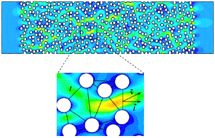
Figure 1: Contour plot of the velocity magnitude for a typical realization of a pore space with porosity $\epsilon=0.7$ subjected to a low Reynolds number and periodic boundary conditions applied in the $y$-direction. The fluid is pushed from left to right. The colors ranging from blue (dark) to red (light) correspond to low and high velocity magnitudes, respectively. The close-up shows a typical pore opening of length $l$ across which the fluid flows with a line average velocity $\vec{v}$. The local flux at the pore opening is given by $q=vl\cos\theta$, where $\theta$ is the angle between $\vec{v}$ and the vector normal to the line connecting the two disks.

First we analyze the geometry of our random configurations making a Voronoi construction of the point set given by the centers of the disks Voronoi08 ; Watson81 . We define two disks to be neighbors of each other if they are connected by a bond of the Voronoi tessellation. These bonds constitute therefore the openings or pore channels through which a fluid can flow when it is pushed through our porous medium, as can be seen in the close-up of Fig. 1. We measure the channel widths $l$ as the length of these bonds minus the diameter $D$ and plot in Fig. 2 the (normalized) distributions of the normalized channel widths $l^{*}=l/D$ for the four different porosities. Clearly one notices two distinct regimes: (i) for large widths $l^{*}$ the distribution decays seemingly exponentially with $l^{*}$, and (ii) for small $l^{*}$ it has a strong dependence on the porosity, increasing dramatically at the origin with decreasing porosity.

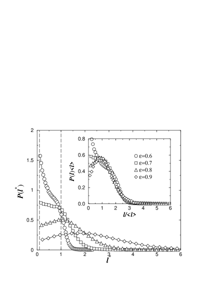
Figure 2: Distributions of the normalized channel widths $l^{*}=l/D$ for different values of porosity $\epsilon$. From left to right, the two vertical dashed lines indicate the values of the minimum distance between disks $l^{*}=0.1$ and the size of the disks $l^{*}=1$. The inset shows the data collapse obtained by rescaling the distributions with $\langle l\rangle$ using Eq. (2).

A closer investigation shows that in Fig. 2 the large $l^{*}$ tail decays like a Gaussian for large porosities while it is a simple exponential when the porosity is around or below $0.7$. The crossover between the two regimes is visible as a peak which shifts between $\epsilon=0.9$ and $0.8$ and then stays for smaller porosities at about $l^{*}=1$, i.e., $l=D$. These distribution functions can be qualitatively understood in the following way. For very large porosities, i.e., very dilute systems, the distance between the particles is essentially uncorrelated due to excluded volume and is therefore Gaussian distributed around a mean value $\langle l\rangle$. If for simplicity one imagines particles being on a regular triangular lattice as an idealized configuration in two dimensions, the following expression is obtained:

$$\langle l\rangle=D(\sqrt{{\pi\over 2\sqrt{3}(1-\epsilon)}}-1)~{}.$$ (2)

The filling process will strongly feel the clogging due to excluded volume when one disk just fits into the hole between three disks. This situation occurs when $\langle l\rangle=D(\sqrt{3}-1)$. Inserting this into Eq. (2) gives a crossover porosity of $\epsilon=1-\pi/6\sqrt{3}\approx 0.7$ which agrees with our simulation (see Fig. 2). Interestingly, a related property, namely the correlation function, does not seem to show such a crossover Torquato95 ; Rintoul96 . The inset of Fig. 2 shows that, for sufficiently large values of $l$, all distributions $P(l)$ collapse to a single curve when rescaled by the corresponding value of $\langle l\rangle$ calculated from Eq. (2). As shown in the inset of Fig. 3, the variation of the average value $\langle l^{*}\rangle$ with porosity follows very closely Eq. (2). Only the prefactor is different from unity ($\approx 1.2$) due to the presence of disorder. This result indicates that our simple description based on a diluted system of particles placed on a regular lattice provides a good approximation for the geometry of the disordered porous medium.

The fluid mechanics in the porous space is based on the assumption that a Newtonian and incompressible fluid flows under steady-state conditions. The Navier-Stokes and continuity equations for this case reduce to

$$\rho~{}{\vec{u}\cdot\nabla\vec{u}}=-{\nabla p}+\mu~{}{\nabla}^{2}{\vec{u}}~{},$$ (3)

$${\nabla\cdot\vec{u}}=0~{},$$ (4)

where $\vec{u}$ and $p$ are the local velocity and pressure fields, respectively, and $\rho$ is the density of the fluid. No-slip boundary conditions are applied along the entire solid-fluid interface, whereas a uniform velocity profile, $u_{x}(0,y)=V$ and $u_{y}(0,y)=0$, is imposed at the inlet of the channel. For simplicity, we restrict our study to the case where the Reynolds number, defined here as $Re\equiv{\rho VL_{y}/\mu}$, is sufficiently low ($Re<1$) to ensure a laminar viscous regime for fluid flow. We use FLUENT Fluent , a computational fluid dynamic solver, to obtain the numerical solution of Eqs. (3) and (4) on a triangulated grid of up to hundred thousand points adapted to the geometry of the porous medium.

Simulations have been performed by averaging over $10$ different pore space realizations generated for each value of porosity. The contour plot in Fig. 1 of the local velocity magnitude for a typical realization of the porous medium with porosity $\epsilon=0.7$ clearly reveals that the transport of momentum through the complex geometry generates preferential channels Andrade99 . Once the numerical solution for the velocity and pressure fields in each cell of the numerical grid is obtained, we compute the fluid velocity magnitudes $v$ associated to each channel. This value is the magnitude of the line average velocity vector $\vec{v}$ calculated as the average over the local velocity vectors ${\vec{u}}$ along the corresponding channel width $l$.

In Fig. 3 we show the data collapse of all distributions of normalized velocity magnitudes $P(v^{*})$, where $v^{*}=v/V$, obtained by rescaling the variable $v^{*}$ with the corresponding value of $\epsilon^{-2}$. It is also interesting to note that these rescaled distributions follow a typical Gaussian behavior except for very small $v^{*}\epsilon^{2}$, as indicated by the solid line in Fig. 3. In the inset of Fig. 3 we also show that the average interstitial velocity indeed scales with the porosity as $\langle v\rangle\sim\epsilon^{-2}$, confirming the rescaling procedure adopted to obtain the collapse of the distributions $P(v^{*})$ in the main plot of Fig. 3. Plotting for each channel $v$ against $l$ gives a cloud of points which for all considered values of $\epsilon$ results in a rather unexpected least square fit relation of the type $v\sim\sqrt{l}$.

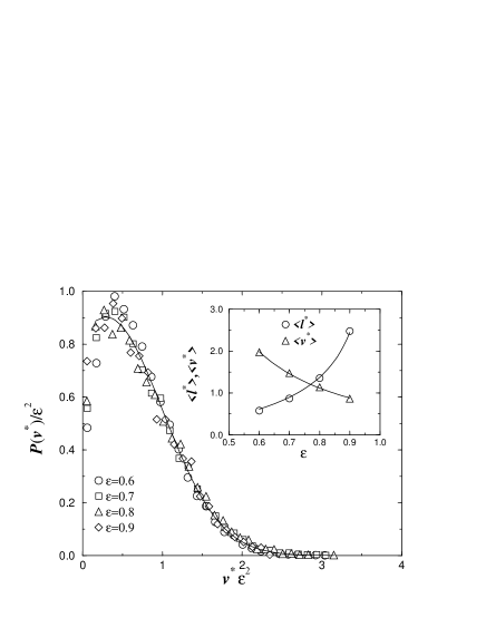
Figure 3: Double-logarithmic plot of the distributions of the local normalized velocity magnitudes $v^{*}$, i.e., $v/V$, multiplied by ${\epsilon}^{2}$ as explained in the text. The solid line is a Gaussian fit. The inset shows the dependence of $\langle l^{*}\rangle$ and $\langle v^{*}\rangle$ on the porosity $\epsilon$. The solid lines are the best fits to the data, corresponding to $\langle l^{*}\rangle=a(\sqrt{b(1-\epsilon)}-1)$, with $a=1.22$ and $b=\pi/2\sqrt{3}$ (see Eq. (2)) and $\langle v^{*}\rangle=0.71\epsilon^{-2}$.

We now analyse the distribution of fluxes throughout the porous medium. Each local flux $q$ crossing its corresponding pore opening $l$ is given by $q=vl\cos\theta$, where $\theta$ is the angle between $\vec{v}$ and the vector normal to the cross section of the channel (see Fig. 1). In Fig. 4 we show that the distributions of normalized fluxes $\phi=q/q_{t}$, where $q_{t}=VL_{y}$ is the total flux, have a stretched exponential form,

$$P(\phi)\sim\exp(-\sqrt{\phi/\phi_{0}})~{},$$ (5)

with $\phi_{0}\approx 0.005$ being a characteristic value. This simple form of Eq. (5) is quite unexpected considering the rather complex dependence of $P(l)$ on $\epsilon$. Moreover, all flux distributions $P(\phi)$ collapse on top of each other when rescaled by the corresponding value of ${\langle l^{*}\rangle}^{-1}\epsilon^{2}$. This collapse for distinct porous media results from the fact that mass conservation is imposed at the microscopic level of the geometrical model adopted here, which is microscopically disordered, but at a larger scale is macroscopically homogeneous Sahimi95 . As also shown in Fig. 4, it is possible to reconstruct the distribution of fluxes using a convolution of the distribution of velocities $v$ and the distribution of oriented channel widths, namely $l{\rm cos}\theta$. Indeed, if we calculate the integral,

$$P(\phi)\!=\!\int\!\int\!P(v)P(l\cos\theta)\delta(\phi-vl\cos\theta)dvd(l\cos\theta)~{},$$ (6)

we find that the original distribution $P(\phi)$ is approximately retrieved, as can also be seen in Fig. 4 (solid line).

Finally, the inset of Fig. 4 shows that the permeability of the two-dimensional porous media closely follows the semi-empirical Kozeny-Carman equation Dullien79 ,

$$\frac{K}{K_{0}}=\kappa\frac{\epsilon^{3}}{(1-\epsilon)^{2}}~{},$$ (7)

where $K_{0}\equiv h^{2}/12$ is a reference value taken as the permeability of an empty channel between two walls separated by a distance $h$. The proportionality constant $\kappa$ is given by the following expression:

$$\kappa\equiv\left(\frac{D}{2h}\right)^{2}\frac{1}{\tau\alpha}~{},$$ (8)

where $\tau\equiv(L_{e}/L)^{2}$ is the hydraulic tortuosity of the porous medium, $\alpha$ corresponds to the pore shape factor, and $L_{e}$ is an effective flow length Dullien79 . If we now make use of the Dupuit-Forchheimer assumption Dullien79 ,

$$\langle v\rangle=\frac{V}{\epsilon}\left(\frac{L_{e}}{L}\right)~{},$$ (9)

we are led to the conclusion that the tortuosity of our porous medium should also scale as $\tau\sim\epsilon^{-2}$. Considering the validity of the Kozeny-Carman equation (7) and the definition of the constant $\kappa$ from Eq. (8), we obtain as a consequence that the shape factor should behave as $\alpha\sim\epsilon^{2}$.

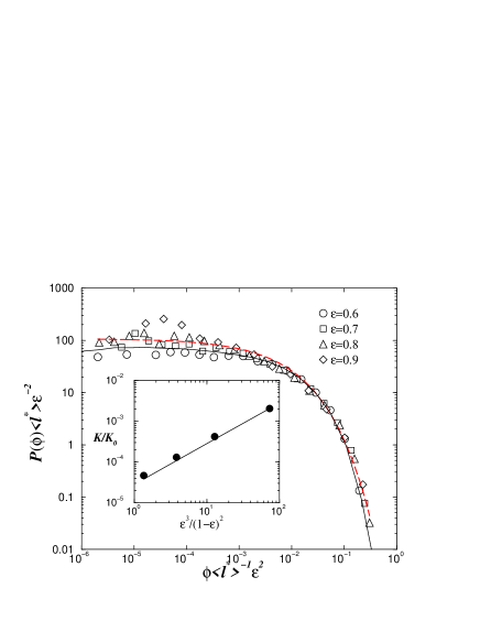
Figure 4: Log-log plot of the distributions of the normalized local fluxes $\phi=q/q_{t}$ for different porosities $\epsilon$. The (red) dashed line is a fit of the form $\exp(-\sqrt{\phi/\phi_{0}})$, where $\phi_{0}\approx 0.005$. The full line stems from the convolution as discussed in the text. In the inset we see a double-logarithmic plot of the global flux and the straight line verifies the Kozeny-Carman equation.

Summarizing we have found that although the distribution of channel widths in a porous medium made by a two-dimensional RSA process is rather complex and exhibits a crossover at $l\sim D$, the distribution of fluxes through these channels shows an astonishingly simple behavior, namely a square-root stretched exponential distribution that scales in a simple way with the porosity. The velocity magnitudes follow a Gaussian distribution truncated at small velocities which scales with the square of the porosity. The distribution of fluxes can be reconstructed as a convolution of the velocity with the channel widths distributions corrected by the velocity orientation factor $\cos\theta$. We propose simple scaling laws for the local fluxes that deepen the understanding of the intrinsic connection between geometrical and flow properties of the random porous medium. Furthermore, we show that our results can be macroscopically described in terms of the Kozeny-Carman relation. Future tasks consist in generalizing these studies to higher Reynolds numbers, three dimensional model of porous media and other types of disorder. Other important challenges are to investigate transient flow and tracer dynamics.

We thank André Moreira, Salvatore Torquato and Bernard Derrida for interesting discussions and the CNPq (CT-PETRO/CNPq), CAPES, FUNCAP, FINEP and the Max Planck Prize for financial support.

References

- (1) F. A. L. Dullien, Porous Media - Fluid Transport and Pore Structure (Academic, New York, 1979).
- (2) P. M. Adler, Porous Media: Geometry and Transport (Butterworth-Heinemann, Stoneham MA, 1992).
- (3) M. Sahimi, Flow and Transport in Porous Media and Fractured Rock (VCH, Boston, 1995).
- (4) S. N. Coppersmith, C.-h. Liu, S. Majumdar, O. Narayan and T. A. Witten, Phys. Rev. E 53, 4673 (1996).
- (5) A. Canceliere, C. Chang, E. Foti, D. H. Rothman, and S. Succi, Phys. Fluids A 2, 2085 (1990).
- (6) S. Kostek, L. M. Schwartz, and D. L. Johnson, Phys. Rev. B 45, 186 (1992).
- (7) N. S. Martys, S. Torquato, and D. P. Bentz, Phys. Rev. E 50, 403 (1994).
- (8) J. S. Andrade Jr., D. A. Street, T. Shinohara, Y. Shibusa, and Y. Arai, Phys. Rev. E. 51, 5725 (1995).
- (9) A. Koponen, M. Kataja, and J. Timonen, Phys. Rev. E 56, 3319 (1997).
- (10) S. Rojas and J. Koplik, Phys. Rev E 58, 4776 (1998).
- (11) J. S. Andrade Jr., U. M. S. Costa, M. P. Almeida, H. A. Makse, and H. E. Stanley, Phys. Rev. Lett. 82, 5249 (1999).
- (12) H. Marshall, M. Sahraoui and M. Kaviany, Phys. Fluids 6, 507 (1993).
- (13) S. Torquato, Random Heterogeneous Materials: Microstructure and Macroscopic Properties (Springer, New York, 2002).
- (14) G. V. Voronoi, J. reine angew. Math. 134, 198 (1908).
- (15) D. F. Watson, The Computer Journal 24, 167 (1981).
- (16) S. Torquato, Phys. Rev. E 51, 3170 (1995).
- (17) M. D. Rintoul, S. Torquato and G. Tarjus, Phys. Rev E 53, 450 (1996).
- (18) FLUENT (trademark of FLUENT Inc.) is a commercial package for computational fluid dynamics.