The Backbone of a City

Abstract

Recent studies have revealed the importance of centrality measures to analyze various spatial factors affecting human life in cities. Here we show how it is possible to extract the backbone of a city by deriving spanning trees based on edge betweenness and edge information. By using as sample cases the cities of Bologna and San Francisco, we show how the obtained trees are radically different from those based on edge lengths, and allow an extended comprehension of the “skeleton” of most important routes that so much affects pedestrian/vehicular flows, retail commerce vitality, land-use separation, urban crime and collective dynamical behaviours.

Centrality is a fundamental concept in network analysis. The issue of structural centrality was introduced in the 40’s in the context of social systems, where it was assumed a relation between the location of an individual in the network and its influence in group processes wasserman94 . Since then, various measures have been proposed over the years to quantify the importance of nodes and edges of a graph, and the concept of centrality have found many applications also in biology and technology bareport ; newmanreview ; vespignanibook ; report .

In economic geography as well as in regional planning, centrality has been dominating the scene especially since the Sixties and Seventies stressing the idea that some places (cities, settlements) are more important than others because they are more “accessible”, where accessibility was intended as a centrality measure of the same kind of those developed in the field of structural sociology, with the difference that the geographic nature of elements in space was saved around a notion of metric distance wilson2000 . In the field of urban design, a long-term effort has been spent in order to understand what urban streets and routes would constitute the “skeleton” of a city, which means the chains of urban spaces that are most important for both the connectedness, liveability and safety at the local scale hillier84 ; hillier96 and its legibility in terms of human wayfinding burgess99 ; more recently, these latter two approaches are seemingly merging together in the first clues of a cognitive/configurational theory penn03 . After an in-depth investigation of both the topological (dual) porta_epb1 and spatial (primal) portacentrality ; porta_epb2 graph representation of street networks, in this paper we provide a tool for the analysis of the backbone of a complex urban system represented as a spatial (planar) graph. Such a tool is based on the mathematical concept of spanning trees, and on the efficiency of centrality measures in capturing the essential edges of a graph. Differently from previous applications of this same concept tree_bet , we consider spatial networks instead of topological ones, so that our trees can be shown graphically on the city maps and can serve as a support in urban design and planning; moreover, we consider two different kinds of edge centrality measures, and we compare the obtained trees with the standard spanning trees based on minimizing the total lengths.

In our approach, cities are represented as spatial networks (networks embedded in the real space), i.e. networks whose nodes occupy a precise position in a two-dimensional Euclidean space, and whose edges are real physical connections report ; west95 . In such approach, 1-square mile samples of urban street patterns selected from Ref. jacobs are transformed into spatial undirected graphs by mapping the intersections into the graph nodes and the roads into links between nodes portacentrality ; porta_epb2 . Here we will focus, in particular, on the cities of Bologna and San Francisco as examples of two different classes of urban street patterns, the former being a self-organized organic network evolved over a long period of time through the uncoordinated contribution of countless historical agents while the latter being a mostly planned fabric built in a relatively short period of time following the ideas of one coordinating historical agent. Each of the two obtained graphs is denoted as $G\equiv G(N,K)$, where $N$ and $K$ are, respectively, the number of nodes and links in the graph. In the case of Bologna we have $N=541$ and $K=773$, while in the case of San Francisco the same amount of 1-square mile of land contains only $N=169$ and $K=271$ edges. The average degree $<k>=2K/N$ is respectively equal to 2.71 and 3.21. This difference is due to the overbundance of three-roads intersections with respect to four-roads intersections in the city of Bologna. The converse is true for the city of San Francisco, due to its square-grid structure. See Ref. cardillo for a plot of the entire degree distributions in the two cases. The graph nodes are characterized by their positions in the unit square $\{x_{i},y_{i}\}_{i=1,...,N}$, while the links follow the footprints of real streets and are associated a set of real positive numbers representing the street lengths, $\{l_{\alpha}\}_{\alpha=1,...,K}$. Another relevant difference between the two cities is captured by the edges length distribution. In Fig. 1 we plot $n(l)$, the number of edges of length $l$, as a function of $l$. The edges length distribution has a single peak in Bologna, while it has more than one peak in a mostly planned cities as San Francisco, due to its grid pattern. In the following, the graph representing a city is described by the adjacency $N\times N$ matrix $A$, whose entry $a_{ij}$ is equal to 1 when there is an edge between $i$ and $j$ and 0 otherwise, and by a $N\times N$ matrix $L$, whose entry $l_{ij}$ is the value associated to the edge $\alpha\equiv(i,j)$, in our case the metric length of the street connecting $i$ and $j$.

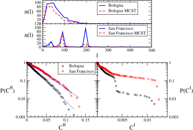
Figure 1: Top panels: the length distributions for the two cities of Bologna and San Francisco (full lines) are compared with the length distributions of the respective betweenness-based MCSTs (dashed lines). The quantity $n(l)$ is defined as the number of edges whose length is in the range [l - 5 meters, l + 5 meters]. Bottom panels: cumulative distributions of edge betweenness $C^{B}$ (left) and information $C^{I}$ (right) for Bologna (circles) and San Francisco (squares). The dashed lines in the left panel are exponential fits to the betweenness distributions.

In a previous work portacentrality , different measures of node centrality centrality ; lm05a , properly extended for spatial graphs, have been investigated in the same database of urban street patterns. Here we show how to construct spanning trees based on edge centrality. We first localize high centrality edges, namely the streets that are structurally made to be traversed (betweenness centrality) or the streets whose deactivation affects the global properties of the system (information centrality). Of course other definitions of edge centrality (as for instance range, closeness or straightness centrality ) can be used as well. The definitions of edge betweenness and edge information we adopt are obvious modifications of the centrality measures defined on nodes.

The edge betweenness centrality, $C^{B}$, is based on the idea that an edge is central if it is included in many of the shortest paths connecting couples of nodes. The betweenness centrality of edge $\alpha=1,...,K$ is defined as ng04 :

$$C^{B}_{\alpha}=\frac{1}{(N-1)(N-2)}\sum_{j,k=1,..,N;j\neq k\neq i}\frac{n_{jk}(\alpha)}{n_{jk}}$$ (1)

where $n_{jk}$ is the number of shortest paths between nodes $j$ and $k$, and $n_{jk}(\alpha)$ is the number of shortest paths between nodes $j$ and $k$ that contain edge $\alpha$.

The edge information centrality, $C^{I}$, is a measure relating the edge importance to the ability of the network to respond to the deactivation of the edge itself. The network performance, before and after a certain edge is deactivated, is measured by the efficiency of the graph $G$ lm01 ; lm03 . The information centrality of edge $\alpha$ is defined as the relative drop in the network efficiency caused by the removal from $G$ of the edge $\alpha$ portacentrality ; lm05a :

$$C^{I}_{\alpha}=\frac{\Delta E}{E}=\frac{E[G]-E[G^{\prime}]}{E[G]}$$ (2)

where the efficiency of a graph $G$ is defined as:

$$E[G]=\frac{1}{N(N-1)}{{\sum_{{i,j=1,..,N;i\neq j}}}\frac{d^{Eucl}_{ij}}{d_{ij}}}$$ (3)

and where $G^{\prime}$ is the graph with $N$ nodes and $K-1$ edges obtained by removing edge $\alpha$ from the original graph $G$. An advantange of using the efficiency instead of the characteristic path length $L$ ws98 to measure the performance of a graph is that $E[G]$ is finite even for disconnected graphs.

In Fig. 1 we report the cumulative distributions of edge betweenness and information. The cumulative distribution $P(C)$ is defined as:

$$P(C)=\int_{C}^{+\infty}\frac{n(C^{\prime})}{K}dC^{\prime}$$ (4)

where $n(C)$ is the number of edges with centrality equal to $C$. The edge distributions are quite similar in the two cities of Bologna and San Francisco. In particular, the betweenness distributions are well fitted by exponential curves, $P(C^{B})\sim exp(-C^{B}/s)$, with coefficients respectively equal to $s_{Bo}=0.020$ and $s_{SF}=0.029$. Thus, for the edge betweenness, the distributions found are similar (single-scale) to those observed for the node betweenness. Conversely, the edge information distributions have not a well defined shape: although their decay is slower than exponential in both Bologna and San Francisco, the edge information distributions do not allow to differentiate self-organized cities from planned ones, as it was instead possible by means of the node information distributions portacentrality . This indicates that there are important correlations in the information centrality of edges incident in the same node. This also indicates that organic self-organized cities are different from planned ones, more in terms of their nodes (intersections) than of their edges (streets), and especially about how they assign importance to such spaces.

We are finally ready to build the Maximum Centrality Spanning Trees (MCSTs), i.e. maximum weight spanning trees where the edge weight is defined as the centrality of the edge. A graph $G^{\prime}(N^{\prime},K^{\prime})$ is a tree if and only if it satisfies any of the following four conditions: 1) $G^{\prime}$ has $N^{\prime}-1$ edges and no cycles; 2) $G^{\prime}$ has $N^{\prime}-1$ edges and is connected; 3) exactly one simple path connects each pair of nodes in $G^{\prime}$; 4) $G^{\prime}$ is connected, but removing any edge disconnects it. Given a connected, undirected graph $G(N,K)$, a spanning tree $T$ is a subgraph of $G$ which is a tree and connects all the $N$ nodes together. Consequently $T\equiv T(N,N-1)$. A single graph can have many different spanning trees. We can also assign a weight $w_{\alpha}$ to each edge $\alpha$, which is usually a number representing how favorable (for instance how central) the edge is, and assign a weight to a spanning tree by computing the sum of the weights of the edges in that spanning tree. A maximum weight spanning tree is then a spanning tree with weight larger than or equal to the weight of every other spanning tree of the graph. It appears evident that it is possible to define appropriate edge weights with the aim of finding particular structures capable of connecting every single node of the graph while minimizing the corresponding total weight. In particular, for each city we have computed two different MCSTs, respectively based on betwenness and information. The two cases are obtained by respectively fixing $w_{\alpha}=C^{B}_{\alpha}$ and $w_{\alpha}=C^{I}_{\alpha}$, with $\alpha=1,...,K$. Since the two centrality measures focus on different properties of the network, using both of them allows us to enforce our analysis.

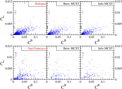
Figure 2: Scatter plots showing the correlations between edge betweenness and edge information in Bologna (top panels) and San Francisco (bottom panels). Each point represents one edge in the orginal graph (left), in the betweenness-based MCST (center), and in the information-based MCST (right).

Moreover, as shown in Fig. 2 left panels, $C^{B}$ and $C^{I}$ are correlated, although it is possible to find edges with a low value of $C^{B}$ and a high $C^{I}$ (and viceversa). The coefficients of linear correlation are respectively equal to $r=0.69$ and $r=0.46$. For the computation of the MCSTs (and of the mLSTs) we have used the Prim’s algorithm cormen that allows to obtain the result in a time proportional to $K\log N$. The MCST for the city of Bologna contains $K^{\prime}=N-1=540$ links, i.e. $70\%$ of the links of the original graph, while the MCST for San Francisco has $K^{\prime}=168$, i.e. $62\%$ of the links of the original graph. Since the links have been chosen according to their centrality values, it turns out that the set of selected edges in the betweenness-based MCST of Bologna (San Francisco) possesses the $86\%$ ( $82\%$) of the total betweenness centrality of the original graph, defined as $\sum_{\alpha=1,K}C^{B}_{\alpha}$ tree_bet . Similarly, the set of selected edges in the information-based MCST of Bologna (San Francisco) possesses the $84\%$ ($95\%$) of the total information centrality. This is both due to the shapes of the centrality distributions shown in Fig. 1 and to the edge selection that avoids, in the tree construction, the formation of cycles. The values of $C^{B}$ and $C^{I}$ for the selected edges are shown in the scatter plots of Fig. 2. In the case of Bologna, the two measures of centrality have the same correlations as in the original graph (the correlation coefficients in the MCST are $r^{B}=0.61$ and $r^{I}=0.64$). Conversely, in San Francisco, the two variables are less correlated in the MCSTs ($r^{B}=0.10$ and $r^{I}=0.29$) than in the original graph ($r=0.46$). In Fig. 1 (top panels) we have plotted the edge length distributions of the betweenness-based MCSTs (dashed lines). It is interesting to observe that, for the city of Bologna, $n(l)$ has the same shape both in the original graph and in its betweenness-based MCST. This means that, in the construction of the tree, edges with all lengths have been removed (with same probability) from the original graph. Conversely, in San Francisco most of the edges not included in the betweenness-based MCST are those with the largest length. The same result has been found for the information-based MCSTs and seems to be a common characteristic of other planned grid-like cities.

In Fig.3 we compare graphically the two MCSTs with the minimum length spanning trees cormen . In the construction of the latter, the weight $w_{\alpha}$ associated to each edge $\alpha$ is set to be equal to the length of the edge $l_{\alpha}$ and represent the cost of the edge. A Minimum Length Spanning Tree (mLST) is then a spanning tree with weight (cost) smaller than or equal to the weight of every other spanning tree of the graph.

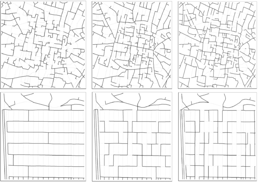
Figure 3: Spanning trees of Bologna (above) and San Francisco (below). From left to right, mLSTs, betweenness-based and information-based MCSTs

The MCSTs obtained are different from the mLSTs. In the case of Bologna, the betweenness (information) based MCST has a total length equal to 1.15 (1.14) times the total length of the mLST, while in the case of San Francisco this ratio is equal to 1.15 (1.07). In the case of Bologna, the MCST based on betweenness (information) has $82\%$ ($75\%$) of the edges in common with the mLST, while in San Francisco it has $70\%$ ($76\%$) of the edges in common with the mLST. It is worth noting that the two MCSTs have $77\%$ of the edges in common in Bologna, whereas such a percentage is smaller in San Francisco ($66\%$). The graphical visualization of the maximum centrality trees is of interest for urban planners since the trees express the uninterrupted chain of urban spaces that serves the whole system while maximizing centrality over all edges involved. This method identifies the backbone of a city system as the sub-network of spaces that are most likely to offer the highest potential for the life of the urban community in terms of popularity, safety and services locations, all factors geographically related with central places. This is evident in Fig. 3, where the comparison between the trees in the two cities clearly indicates that the spatial sub-system that keeps together a city in terms of the shortest trip length is not the same spatial sub-system that does it in terms of the highest centrality. It is also worth noting that metric distance is also involved in the algorithms for the calculation of centrality indices, so that all kinds of trees considered hereby are rooted in the geographic space. The second thing is that while the shortest length backbone performs effectively when applied to planned urban fabrics like San Francisco, in self-organized evolutionary cases like that of Bologna it does not individuates continuous routes nor clearly distinguishes a hierarchy of sub-systems in the network, while the highest information and especially the highest betweenness backbones do. In a way, we would say that organic patterns are more oriented to put things and people together in public space than to shorten the trips from any origin to any destination in the system, this latter character being more typical of planned cities.

In conclusion, in this work we have shown that the concept of MCST leads to a meaningful picture of the primary sub-system of a city network, which makes it a single component while minimizing the cost of moving around and maximizing the potential of places to achieve social success, safety and popularity. Therefore, the method has the potential of becoming an useful tool in city planning and design, due to its immediate and powerful visualization outcome.

Acknowledgment. We thank P. Crucitti for many helpful discussions and suggestions.

References

- (1) S. Wasserman and K. Faust, Social Networks Analysis, (Cambridge University Press, Cambridge, 1994).
- (2) R. Albert and A.-L. Barabási, Rev. Mod. Phys. 74, 47 (2002).
- (3) M.E.J. Newman, SIAM Review 45, 167 (2003).
- (4) R. Pastor-Satorras, A. Vespignani, Evolution and Structure of the Internet: A Statistical Physics Approach, (Cambridge University Press, 2004).
- (5) S. Boccaletti, V. Latora, Y. Moreno, M. Chavez and D.-U. Hwang, Phys. Rep. in press.
- (6) G.A. Wilson, Complex spatial systems: the modelling foundations of urban and regional analysis, (Prentice Hall, Upper Saddle River, NJ, 2000).
- (7) B. Hillier and J. Hanson The social logic of space (Cambridge University Press, Cambridge, UK, 1984).
- (8) B. Hillier Space is the machine: a configurational theory of architecture (Cambridge University Press, Cambridge, UK, 1996).
- (9) N. Burgess, K.J. Jeffery, O’Keefe J (eds.), The hippocampal and parietal foundations of spatial cognition , (OUP, Oxford, UK, 1999).
- (10) A. Penn, Environment and Behavior 35, 30 (2003).
- (11) S. Porta, P. Crucitti and V. Latora, Preprint cond-mat/0411241.
- (12) P. Crucitti, V. Latora and S. Porta, Preprint physics/0504163.
- (13) S. Porta, P. Crucitti and V. Latora, Preprint physics/0506009. In Press in Environment and Planning B
- (14) D. Kim, J.D. Noh, and H. Jeong, Phys. Rev. E70, 046126 (2004)
- (15) D.B. West, Introduction to Graph Theory, (Prentice Hall, 1995).
- (16) A. Jacobs, Great streets (MIT Press, Boston, MA, 1993).
- (17) A. Cardillo, S. Scellato, V. Latora and S. Porta, Preprint physics/0510162
- (18) V. Latora and M. Marchiori, Preprint cond-mat/0402050
- (19) V. Latora and M. Marchiori, Phys. Rev. E71, 015103(R) (2005).
- (20) M. E. J. Newman and M. Girvan, Phys. Rev. E69, 026113 (2004).
- (21) V. Latora and M. Marchiori, Phys. Rev. Lett. 87, 198701 (2001).
- (22) V. Latora and M. Marchiori, Eur. Phys. J. B32, 249 (2003).
- (23) I. Vragovic, E. Louis, A. Diaz-Guilera, Phys. Rev. E71, 036122 (2005).
- (24) D.J. Watts and S.H. Strogatz, Nature 393, 440 (1998).
- (25) T.H. Cormen, C.E. Leiserson, R.L. Rivest, C. Stein, Introduction to Algorithms (MIT University Press, Cambrdige, 2001).