Abstract

The accurate determination of atomic masses and the high-precision measurement of the bound-electron $g$ factor are prerequisites for the determination of the electron mass, which is one of the fundamental constants of nature. In the 2002 CODATA adjustment [P. J. Mohr and B. N. Taylor, Rev. Mod. Phys. 77, 1 (2005)], the values of the electron mass and the electron-proton mass ratio are mainly based on $g$ factor measurements in combination with atomic mass measurements. In this paper, we briefly discuss the prospects for obtaining other fundamental information from bound-electron $g$ factor measurements, we present some details of a recent investigation of two-loop binding corrections to the $g$ factor, and we also investigate the radiative corrections in the limit of highly excited Rydberg $S$ states with a long lifetime, where the $g$ factor might be explored using a double resonance experiment.
PACS Nos.: 31.30.Jv, 12.20.Ds, 11.10.St
Keywords: Quantum Electrodynamics; Bound States; Atomic Physics.

1 Introduction

The central equation for the determination of the electron mass $m_{\rm e}$ from $g$ factor measurements reads

$$m_{\rm e}=\frac{\omega_{\rm c}}{\omega_{\rm L}}\,\frac{g\,|e|}{2q}\,m_{\rm ion}\,,$$ (1)

where $\omega_{\rm c}$ is the cyclotron frequency of the ion, $\omega_{\rm L}$ the Larmor spin precession frequency, $q$ the ion charge, and $m_{\rm ion}$ its mass. The quantity $e=-|e|$ is the elementary charge, and $g$ is the bound-electron $g$ factor. In most practical applications, the ion is hydrogenlike, and the frequency ratio $\omega_{\rm c}/\omega_{\rm L}$ can be determined very accurately in a Penning trap [1, 2].

Equation (1) may now be interpreted in different ways:

• The ratio $m_{\rm e}/m_{\rm ion}$ is immediately accessible, provided we assume that quantum electrodynamic theory holds for $g$. Provided the ratio $m_{\rm ion}/m_{\rm p}$ (with the proton mass $m_{\rm p}$) is also available to sufficient accuracy, the electron to proton mass ratio $m_{\rm e}/m_{\rm p}$ can be determined by multiplication $m_{\rm e}/m_{\rm ion}\times m_{\rm ion}/m_{\rm p}$. In the recent CODATA adjustment [3], the ratio $m_{\rm e}/m_{\rm p}$ has been determined using two measurements involving ${}^{12}{\rm C}$.

• Let us suppose that $m_{\rm ion}$ is known to sufficient accuracy. Assuming that quantum electrodynamic theory holds for $g$, we may then determine $m_{\rm e}$ from the measurement [4, 5, 6].

• The $g$ factor depends on the reduced mass of the electron-ion two-particle system. An accurate measurement of $g$ can therefore yield an independent verification of the isotopic nuclear mass difference, provided that the masses of the ions have been determined beforehand to sufficient accuracy [7].

• Direct access to the electron $g$ factor in a weak external magnetic field depends on the property of the nucleus having zero spin. According to a relatively recent proposal [8, 9], the measurement of a $g$ factor for a nucleus with non-zero spin can be used to infer the nuclear $g$ factor, provided the purely electronic part of the $g$ factor is known to sufficient accuracy from other measurements.

• There is also a proposal for measuring $g$ factors in lithiumlike systems, and theoretical work in this direction has been undertaken [10]. Provided the contribution due to electron-electron correlation can be tackled to sufficient accuracy, a measurement of the $g$ factor in lithiumlike systems could give access to the nuclear-size effect, which in turn can be used as an additional input for other determinations of fundamental constants.

• Finally, provided the mass $m_{\rm ion}$ of a high-$Z$ ion is known to sufficient accuracy and $m_{\rm e}$ is taken from $g$ factor measurements at lower nuclear charge number, the high-$Z$ experimental result for $g$ may be compared to a theoretical prediction, yielding a test of quantum electrodynamics for a bound particle subject to an external magnetic field and a strong Coulomb field (see, e.g., Sec. 2.2 of [11]). Alternatively, one may invert the relation $g=g(\alpha)$ to solve for the fine-structure constant (important precondition: knowledge of nuclear size effect) [8, 12]. The feasibility of the latter endeavour in various ranges of nuclear charge numbers will be discussed in the current article.

These examples illustrate the rich physics implied by $g$ factor measurements in combination with the determination of atomic masses via Penning traps. Indeed, the $g$ factor is a tremendous source of information regarding fundamental constants, fundamental interactions and nuclear properties.

This paper is organized as follows. In Sec. 2, we briefly discuss the importance and the status of atomic mass measurements for further advances. In Sec. 3, we describe a few details of two recent investigations [5, 6] regarding one- and two-loop binding corrections to the $g$ factor, and in Sec. 4, we discuss the asymptotics of the corrections for high quantum numbers, with a partially surprising result, before dwelling on connections of the $g$ factor to nuclear effects and the fine-structure constant in Sec. 5. Conclusions are drawn in Sec. 6. An Appendix is devoted to the current status of the free-electron anomaly.

2 Atomic Mass Measurements – Present and Future

A review of the current status of atomic mass measurements can be in found in Ref. [13]. Experimental details regarding modern atomic mass measurements, with a special emphasis on hydrogenlike ions, can be found in Refs. [14, 15]. Regarding the current status of mass measurements, one may point out that some of the masses of S, Kr and Xe ions have recently been determined with an accuracy of better than 1 part in $10^{10}$ (Ref. [16]). For molecular ions, the accuracy has recently been pushed below $10^{-11}$ [17].

Recent measurements for the hydrogenlike ions ${}^{24}{\rm Mg}^{11+}$ and ${}^{26}{\rm Mg}^{11+}$ (Ref. [14]) and ${}^{40}{\rm Ca}^{19+}$ (Ref. [18]), as well as for the lithiumlike ion ${}^{40}{\rm Ca}^{17+}$ (Ref. [18]) have reached an accuracy of about $5\times 10^{-10}$. These experiments pave the way for accurate determinations of fundamental constants using $g$ factor measurements in these systems. At the University of Mainz [19] (MATS collaboration) and at the University of Stockholm [18] (SMILE-TRAP), there are plans to significantly extend and enhance atomic mass measurements (including many more isotopes and nuclei) over the next few years, with accuracies below 1 part in $10^{11}$ or even $10^{12}$. Eventually, one may even hope to determine the nuclear size effect of a specific ion by “weighing” the Lamb shift of the ground state. In the same context, one may point out that the masses of different charge states of ions are determined vice versa by adding and subtracting binding energies. This implies, e.g., that the mass of ${}^{12}{\rm C}^{5+}$ in terms of the mass of neutral carbon, $m({}^{12}{\rm C})=12\,{\rm u}$, is given by

$$m({}^{12}{\rm C}^{5+})=m({}^{12}{\rm C})-5\,m_{\rm e}+c^{-2}\,E_{\rm B}\,,$$ (2)

where $E_{\rm B}=579.835(1)\times 10^{-9}\,{\rm u}c^{2}$ is the cumulative binding energy for all 5 electrons [20]. This relation has proven useful in the determination of the electron mass [7].

In order to make a comparison to the accuracy of the free-electron determination of $\alpha$, it is perhaps useful to remember that in the seminal work [21], the free-electron and positron anomaly has been determined to an accuracy $4\times 10^{-9}$. This translates into a level of accuracy of about $4\times 10^{-12}$ for the $g$ factor itself. The accuracy of the current value of $\alpha$ is $4\times 10^{-9}$ [3].

3 Calculation of the Bound–Electron $g$ Factor

The bound-electron $g$ factor measures the energy change of a bound electron (hydrogenlike ion, spinless nucleus) under a quantal change in the projection of the total angular momentum with respect to an axis defined by a (weak) external magnetic field. In this sense, the $g$ factor of a bound electron should rather be termed the $g_{J}$ factor (according to the Landé formulation).

However, for $S$ states, the total angular momentum number is equal to the spin quantum number, and therefore it has been common terminology not to distinguish the notation for $g$ and $g_{J}$.

For a general hydrogenic state, the Dirac-theory $g$ factor, denoted $g_{\rm D}$, reads (see [9] and references therein)

$$g_{\rm D}=\frac{\kappa}{j(j+1)}\,\left(\kappa\,\frac{E_{n\kappa}}{m_{\rm e}}-\frac{1}{2}\right)\,.$$ (3)

Here, $E_{nj}$ is the Dirac energy, and the quantum numbers $n$, $j$ and $\kappa$ have their usual meaning. Throughout this article, we use natural units with $\hbar=c=\epsilon_{0}=1$.

For $S$, $P$ and $D$ states, Eq. (3) leads to the following expressions (we here expand the bound-state energy in powers of $Z\alpha$),

$$g_{\rm D}(nS_{1/2}) = 2-\frac{2\,(Z\alpha)^{2}}{3\,n^{2}}-\frac{(Z\alpha)^{4}}{n^{3}}\,\left(\frac{2}{3}-\frac{1}{2\,n}\right)\,,$$ (4a)

$$g_{\rm D}(nP_{1/2}) = \frac{2}{3}-\frac{2\,(Z\alpha)^{2}}{3\,n^{2}}-\frac{(Z\alpha)^{4}}{n^{3}}\,\left(\frac{2}{3}-\frac{1}{2\,n}\right)\,,$$ (4b)

$$g_{\rm D}(nP_{3/2}) = \frac{4}{3}-\frac{8\,(Z\alpha)^{2}}{15\,n^{2}}-\frac{(Z\alpha)^{4}}{n^{3}}\,\left(\frac{4}{15}-\frac{2}{5\,n}\right)\,,$$ (4c)

$$g_{\rm D}(nD_{3/2}) = \frac{4}{5}-\frac{8\,(Z\alpha)^{2}}{15\,n^{2}}-\frac{(Z\alpha)^{4}}{n^{3}}\,\left(\frac{4}{15}-\frac{2}{5\,n}\right)\,,$$ (4d)

$$g_{\rm D}(nD_{5/2}) = \frac{6}{5}-\frac{18\,(Z\alpha)^{2}}{35\,n^{2}}-\frac{(Z\alpha)^{4}}{n^{3}}\,\left(\frac{6}{35}-\frac{27}{70\,n}\right)\,.$$ (4e)

The above formulas illustrate the in principle well-known fact that the bound-electron $g$ factor would be different from the free-electron Dirac value $g=2$, even for $S$ states and even in the absence of quantum electrodynamic loop corrections.

We now briefly summarize the results of recent investigations [5, 6] of the bound-electron $g$ factor, which is based on nonrelativistic quantum electrodynamics (NRQED). The central result of this investigation is the following semi-analytic expansion in powers of $Z\alpha$ and $\ln(Z\alpha)$ for the bound-electron $g$ factor ($n{S}$ state) in the non-recoil and pointlike-nucleus limit (for recoil effects see e.g. Ref. [22]):

$$g(n{S}) =\underbrace{2-\frac{2\,(Z\alpha)^{2}}{3\,n^{2}}+\frac{(Z\alpha)^{4}}{n^{3}}\,\left(\frac{1}{2n}-\frac{2}{3}\right)+{\cal O}{(Z\alpha)^{6}}}_{\mbox{Breit (1928), Dirac theory}}$$

$$+\underbrace{{\frac{\alpha}{\pi}}\,\left\{{2\times\frac{1}{2}}\,{\bigg{(}}1+\frac{(Z\alpha)^{2}}{6n^{2}}{\bigg{)}}+\frac{(Z\alpha)^{4}}{n^{3}}{\bigg{\{}}a_{41}\,{\ln}[(Z\alpha)^{-2}]+a_{40}{\bigg{\}}}+{\cal O}(Z\alpha)^{5}\right\}}_{\mbox{one-loop correction}}$$

$$+\underbrace{{\left(\frac{\alpha}{\pi}\right)^{2}}\,\left\{{-0.656958}\,{\bigg{(}}1+\frac{(Z\alpha)^{2}}{6n^{2}}{\bigg{)}}+\frac{(Z\alpha)^{4}}{n^{3}}{\bigg{\{}}b_{41}\,{\ln}[(Z\alpha)^{-2}]+b_{40}{\bigg{\}}}+{\cal O}(Z\alpha)^{5}\right\}}_{\mbox{two-loop correction}}$$

$$+{\cal O}(\alpha^{3})\,.$$ (5)

This expansion is valid through the order of two loops (terms of order $\alpha^{3}$ are neglected). The notation is in part inspired by the usual conventions for Lamb-shift coefficients [23]: the (lower case) $a$ terms denote the one-loop effects, with $a_{kj}$ denoting the coefficient of a term proportional to $\alpha\,(Z\alpha)^{k}\,{\ln}^{j}[(Z\alpha)^{-2}]$. The $b$ terms denote the two-loop corrections, with $b_{kj}$ multiplying a term proportional to $\alpha^{2}\,(Z\alpha)^{k}\,{\ln}^{j}[(Z\alpha)^{-2}]$. In [5, 6], complete results are derived for the coefficients $a_{41}$, $a_{40}$, $b_{41}$ and $b_{40}$, valid for arbitrary excited $S$ states in hydrogenlike systems.

Figure 1: One–loop, two-vertex scattering diagrams that correspond to the one-loop part of the effective operators Eq. (B16) and (B17) of Ref. [6]. The zigzag line denotes the interaction with the external field, whereas the dashed lines denote the Coulomb photons. The two-loop part of these effective operators is generated by diagrams with one more virtual photon, with electron-photon vertices to be inserted at all topologically distinguishable positions in the electron lines of diagrams (a), (b) and (c).

In Eq. (3), the term underlined by “Breit (1928), Dirac theory” corresponds to the prediction of relativistic atomic theory, including the relativistic corrections to the wave function [24]. By contrast, the term $\frac{\alpha}{\pi}\,(2\times\frac{1}{2})$ in the expression underlined by “one-loop correction” gives just the leading (Schwinger) correction to the anomalous magnetic moment of a free electron. This latter effect is modified here by additional binding corrections to the one-loop correction, which give rise e.g. to terms of order $\alpha\,(Z\alpha)^{2}$ and higher (in $Z\alpha$). Perhaps, it is also worth clarifying that the term $-0.656958$ is just twice the two-loop contribution to the anomalous magnetic moment of a free electron, which is usually quoted as $(\frac{\alpha}{\pi})^{2}\,(-0.328479)$ in the literature.

Explicit results for the coefficients in (3), restricted to the one-loop self-energy, read [5]

$$a_{41}(nS) =\frac{32}{9}\,,$$ (6a)

$$a_{40}(nS) =\frac{73}{54}-\frac{5}{24n}-\frac{8}{9}\,\ln k_{0}(n{S})-\frac{8}{3}\,\ln k_{3}(n{S})\,.$$ (6b)

Here, $\ln k_{0}(nS)$ is the Bethe logarithm for an $nS$ state, and $\ln k_{3}(nS)$ is a generalization of the Bethe logarithm to a perturbative potential of the form $1/r^{3}$ (see also Table 1 below). Vacuum polarization adds a further $n$-independent contribution of $(-16/15)$ to $a_{40}$ [25]. Higher-order binding corrections to the one-loop self-energy contribution to the $g$ factor have been considered, e.g., in [26], and for the vacuum-polarization contribution, one may consult, e.g., Ref. [27].

The results for the two-loop coefficients read

$$b_{41}(nS) = \frac{28}{9}\,,$$ (7a)

$$b_{40}(nS) = \frac{258917}{19440}-\frac{4}{9}\,\ln k_{0}-\frac{8}{3}\,\ln k_{3}(nS)+\frac{113}{810}\,{\pi}^{2}-\frac{379}{90}\,{\pi}^{2}\,\ln 2+\frac{379}{60}\,\zeta(3)$$ (7b)

$$+\frac{1}{n}\left(-\frac{985}{1728}-\frac{5}{144}\,{\pi}^{2}+\frac{5}{24}\,{\pi}^{2}\,\ln 2-\frac{5}{16}\,\zeta(3)\right)\,.$$

Our result for $b_{40}$ includes contributions from all two-loop effects (see Fig. 21 of [28] for the diagrams) up to the order $\alpha^{2}\,(Z\alpha)^{4}$. The logarithmic term $b_{41}$ is, however, exclusively related to the two-loop self-energy diagrams. An essential contribution to the one- and two-loop effects is given by two–Coulomb–vertex scattering amplitudes (see also Fig. 1).

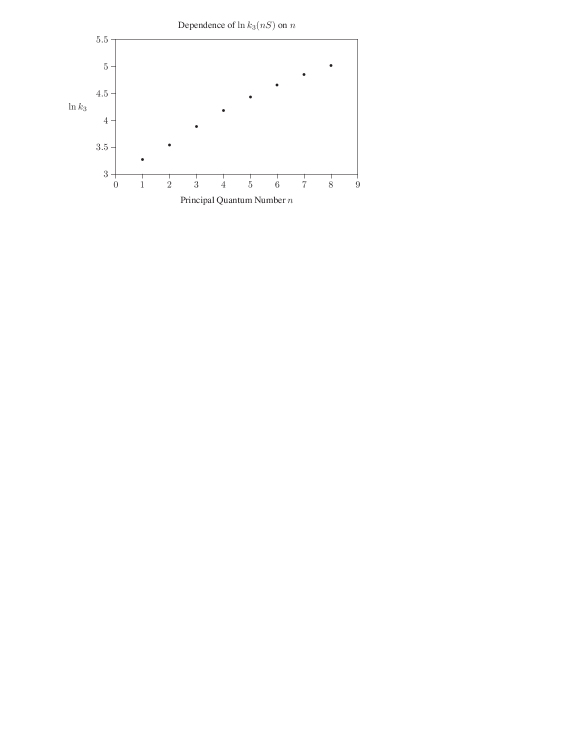
Figure 2: A plot of the generalized Bethe logarithms $\ln k_{3}(nS)$ as a function of the principal quantum number $n$ illustrates the monotonic increase with $n$. For the numerical values, see Table 1.

4 Asymptotics for High Quantum Numbers

It is interesting to study the limit of the coefficients $a_{40}$ and $b_{40}$ in the limit of highly excited states, $n\to\infty$. For the Bethe logarithm $\ln k_{0}$, such a study has recently been completed (see Refs. [29, 30]). The asymptotics of the generalized Bethe logarithm $\ln k_{3}$ have not yet been determined. We here supplement the numerical result for $8S$. In Eq. (72) of Ref. [6], results have been communicated for $S$ states with $n\leq 7$.

Table 1: A table of generalized Bethe logarithms $\ln k_{3}(nS)$ for excited $S$ states. This quantity enters into Eqs. (6b) and (7b) and characterize the one-loop binding correction to the $g$ factor of order $\alpha\,(Z\alpha)^{4}$ and the two-loop correction of order $\alpha^{2}\,(Z\alpha)^{4}$. All decimals shown are significant.

$n$	$\ln k_{3}(nS)$
1	3.272 806 545
2	3.546 018 666
3	3.881 960 979
4	4.178 190 961
5	4.433 243 558
6	4.654 608 237
7	4.849 173 615
8	5.022 275 220

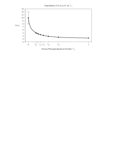
Figure 3: A plot of the generalized Bethe logarithms $\ln k_{3}(nS)$ as a function $1/n$ instead of $n$ indicates consistency with an asymptotic limit $\lim_{n\to\infty}\ln k_{3}(nS)=10\pm 2$.

The result for $n=8$ confirms the trend of a monotonic increase of $\ln k_{3}$ with $n$ (see Fig. 2). On the other hand, based on the general experience regarding the structure of radiative corrections in the limit $n\to\infty$, we would expect a constant limit of $\ln k_{3}(nS)$ for $n\to\infty$. Using an extrapolation scheme similar to the one employed in [31], we conjecture the following limit (see Fig. 3),

$$\lim_{n\to\infty}\ln k_{3}(nS)=10\pm 2\,,$$ (8)

It would be very interesting to verify this limit by an explicit calculation, e.g., using the techniques outlined in Ref. [29].

Highly excited Rydberg states are characterized by a long lifetime. In a Penning trap, however, the confining electric fields would tend to quench transitions to lower-lying levels. One might attempt a measurement of a $g$ factor of a Rydberg state via a double-resonance approach, with one laser driving the spin flip (Larmor precession frequency) and another being tuned to a transition between Rydberg states [32].

5 Bound–Electron $g$ Factor, Nuclear Effects and the Fine–Structure Constant

In Figs. 4 and 5, we indicate three primary sources of the theoretical uncertainty of the bound-electron $g$ factor across the entire range of nuclear charge numbers (these are the fine-structure constant, higher-order unknown two-loop effects and the nuclear radius). For a determination of the fine-structure constant using the bound-electron $g$ factor, the experimental accuracy would have to be improved to a value below the corresponding uncertainty curve in Figs. 4 and 5. Such a determination would constitute a very important and attractive additional pathway, using bound-state quantum electrodynamics, as an alternative to the “usual” determination based on the free-electron $g$ factor.

Before we dwell further on the fine-structure constant, we briefly discuss the nuclear polarizability correction to the $g$ factor (see Ref. [33] and Appendix A) which represents an additional obstacle in the determination of the fine-structure constant from $g$ factor measurements. One might hope that it can be accurately understood one day in terms of nuclear models. In Appendix A, we present an additional nuclear effect (a magnetic susceptibility correction) which may also have to be taken into account in an accurate description of the nuclear contributions to the bound-electron $g$ factor, especially in the range of medium nuclear charge numbers.

The further shift/uncertainty of the $g$ factor, caused by the nuclear finite-size effect (nuclear volume effect), is typically smaller than the uncertainty of the theoretical prediction for the $g$ factor due to higher-order quantum electrodynamic two-loop binding corrections (see Figs. 4 and 5). In evaluating the uncertainty due to the nuclear radius, we have used the most recent values for the root-mean-square (rms) nuclear radii [34].

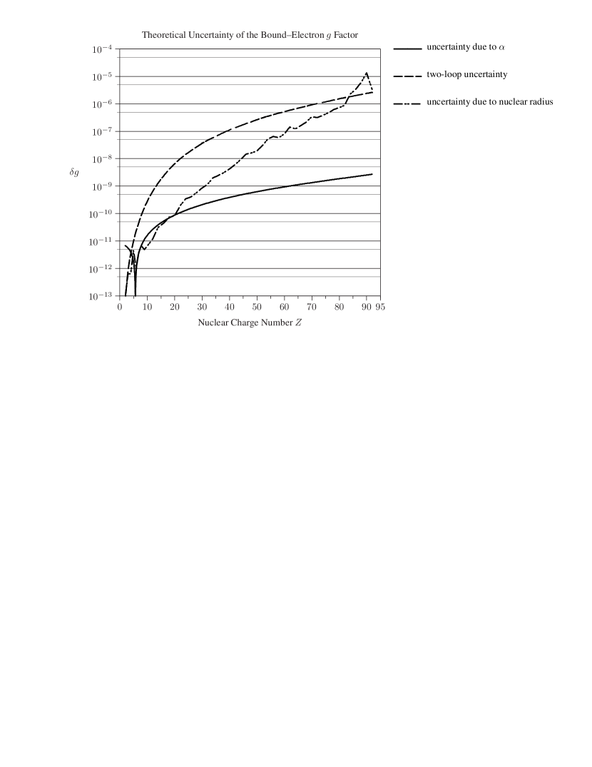
Figure 4: Various sources of theoretical uncertainty for the bound-electron $g$ factor, over the entire $Z$ range from hydrogen to uranium.

In order to investigate the sensitivity of the bound-electron $g$ factor to the fine-structure constant, we approximate the $g$ factor by the first two terms in the $Z\alpha$-expansion of the Dirac theory and the one-loop correction, and obtain

$$\delta g\approx\left\{-\frac{2}{3}\,Z^{2}\,\alpha\,\left[2+(Z\alpha)^{2}\right]+\frac{1}{\pi}\,\left[1+\frac{1}{2}\,(Z\alpha)^{2}\right]\right\}\,\delta\alpha\,.$$ (9)

For a determination of $\alpha$, it is desirable, in principle, to tune the parameters so that the modulus $|\delta g|$ for given $\delta\alpha$ becomes as large as possible.

For nuclear charge numbers in the (fictitious) range $5\leq Z\leq 6$, the sensitivity of $g$ on $\alpha$ suffers from a cancellation of the one-loop against the Dirac binding corrections (see also Figs. 4 and 5), and we have

$$\frac{\delta g}{\delta\alpha}\approx 0\qquad\mbox{for}\qquad Z\approx 5.7\,.$$ (10)

It would be rather difficult to determine $\alpha$ via a measurement of the $g$ factor in the indicated range of nuclear charge numbers.

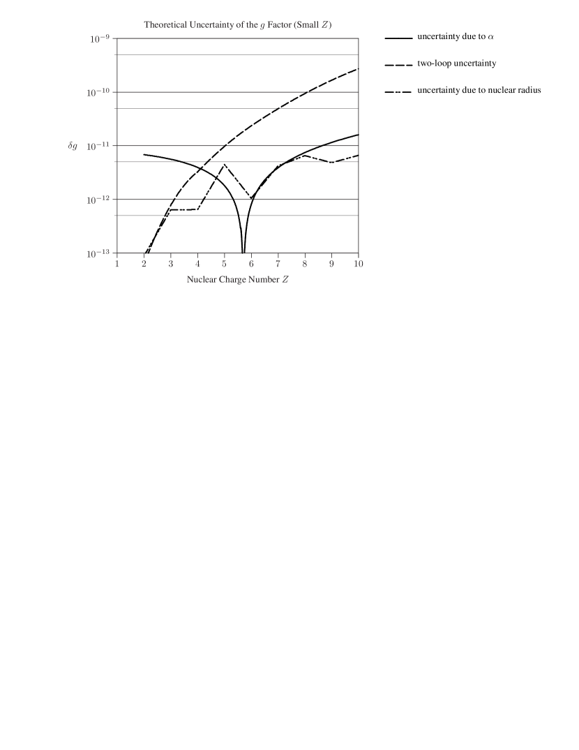
Figure 5: A close-up of Fig. 4 in the range of small quantum numbers $n$ illustrates that an alternative determination of the fine-structure constant, based on the current theoretical status, would be possible for ionized helium (${}^{4}{\rm He}^{+}$) and beryllium (${}^{10}{\rm Be}^{+}$). The ${}^{6,7}{\rm Li}$ nuclei are not spinless.

For large $Z$, one may find a crude approximation to Eq. (9) by the relation

$$\frac{|\delta g|}{\delta\alpha}\approx\frac{4}{3}\,Z^{2}\,\alpha\qquad\Rightarrow\qquad\frac{|\delta g|}{g}\approx\frac{2}{3}\,(Z\,\alpha)^{2}\,\frac{\delta\alpha}{\alpha}\,.$$ (11)

The enhancement of the theoretical uncertainty of $g$ with $Z$ is manifest in Fig. 4. In principle, one might assume that a measurement at high $Z$ could be more favourable for a determination of $\alpha$ than a corresponding experiment in a low-$Z$ system. However, as shown in Fig. 4, the nuclear structure alone currently entails an uncertainty of $g$ that is larger than the uncertainty due to the fine-structure constant, for large $Z$. Also, the uncertainty due to higher-order unknown two-loop binding corrections currently represents an obstacle for an alternative determination of $\alpha$ from a $g$ factor measurement at high $Z$.

Reversing the argument, one may point out that, provided the two-loop uncertainty of the theoretical prediction for large $Z$ can be reduced substantially, one may infer the nuclear radius from the measurement of the $g$ factor. Again, going one step further and assuming that the nuclear radius is accurately known from other measurements, e.g., Lamb shift experiments or $g$ factor measurements in lithiumlike systems, one may eventually hope to infer the fine-structure constant from a high-$Z$ measurement. This endeavour can thus be interpreted as a rather difficult combined effort of theory and experiment, with results not to be expected in the immediate future, but providing a very interesting perspective in the medium and long term. In particular, this endeavour would depend on a successful evaluation, nonperturbative in $Z\alpha$, of all two-loop binding corrections to the bound-electron $g$ factor.

As Fig. 5 shows, the determination of $\alpha$ based on the bound-electron $g$ factor currently appears much more promising for extremely light systems, such as ${}^{4}{\rm He}^{+}$. The measurement of $g$ factor, however, would definitely have to be carried out with an accuracy better than $10^{-11}$ in order to match the current accuracy for $\alpha$. Alternatively (see Fig. 4), the planned $g$ factor measurement in ${}^{40}{\rm Ca}^{19+}$ could potentially lead to a value of $\alpha$ that matches the accuracy of the free-electron value, provided the two-loop uncertainty (higher-order binding corrections) can be reduced and provided the accuracy of the atomic mass determination can be enhanced beyond $10^{-10}$. With current theory, the accuracy of the determination of $\alpha$ from the ${}^{40}{\rm Ca}^{19+}$ measurements is limited to an accuracy of about two orders of magnitude less than the free-electron value.

A final word on the electron mass: For a speculative alternative determination of $\alpha$ in a high-$Z$ experiment, the current accuracy of $m_{\rm e}$, based on the carbon and oxygen measurements [1, 4, 26, 2, 5, 6] is sufficient. We recall the values (evaluated using the most recent theory [6])

$$m_{\rm e}({}^{12}{\rm C}^{5+})= 0.000\,548\,579\,909\,32(29)\,{\rm u}\,,$$ (12)

$$m_{\rm e}({}^{16}{\rm O}^{7+})= 0.000\,548\,579\,909\,60(41)\,{\rm u}\,.$$ (13)

However, if an alternative determination of $\alpha$ via low-$Z$ measurements is pursued in earnest, then it becomes necessary to improve the value of $m_{\rm e}$ beyond the $10^{-11}$ threshold.

6 Conclusions

In Sec. 2, we emphasize the importance of current high-precision and upcoming ultra-high precision atomic mass measurements for the determination of fundamental physical constants, in combination with bound-electron $g$ factor measurements in hydrogenlike systems. One of the celebrated achievements connected to $g$ factor measurements lies in the improvement of the accuracy of the electron mass by a factor of 4, as compared to the previous value based on measurements involving protons and electrons in Penning traps [35].

The expansion of the bound-electron $g$ factor in terms of the two most important parameters in the non-recoil limit is discussed in Sec. 3. These are the loop expansion parameter $\alpha$ (the fine-structure constant) and the Coulomb binding parameter $Z\alpha$, where $Z$ is the nuclear charge number. Furthermore, in Sec. 4, we analyze generalized Bethe logarithms, termed $\ln k_{3}$, which are relevant for binding corrections to the $g$ factor, in the limit of large principal quantum number (i.e., for highly excited Rydberg states). The calculation of the result $\ln k_{3}(8S)=5.022\,275\,220$ (see Table 1), facilitates the analysis of the asymptotic limit. The discussion is accompanied by a tentative proposal [32] for a double-resonance experiment, to probe the bound-electron $g$ factor for highly excited Rydberg states with a long lifetime. In Sec. 5, we discuss prospects for determinations of nuclear properties, and of the fine-structure constant, based on measurements in various ranges of the nuclear charge number. An alternative measurement of the fine-structure constant, of comparable accuracy to the free-electron value, could be accomplished via measurements at low $Z$, provided the experimental accuracy of the $g$ factor can be pushed beyond 1 part in $10^{11}$, and provided the electron mass can be determined to sufficient accuracy (see also Figs. 4 and 5). A priori, combined ultra-high precision measurements in ${}^{4}{\rm He}^{+}$ and ${}^{10}{\rm Be}^{3+}$ appear to provide for a viable approach, provided the atomic mass measurements of ${}^{4}{\rm He}$ and ${}^{10}{\rm Be}$ can reach comparable accuracy (now, the experimental accuracy stands at $1.5$ parts in $10^{11}$ for ${}^{4}{\rm He}$, see Ref. [13]). The two measurements in He and Be could provide input data for a coupled system of equations, to be solved for $\alpha$ and $m_{\rm e}$.

By contrast, considerable further theoretical and experimental progress (concerning, e.g., nuclear radii) is required before any such endeavour could be realized in the domain of high nuclear charges. The prerequisites are outlined in Sec. 5. We conclude that even in the absence of this progress, prospective measurements at higher $Z$ will yield a rather interesting verification of quantum electrodynamics in the high-field domain.

Appendix A Nuclear Magnetic Susceptibility Correction

It is well recognized that the nuclear polarizability can shift atomic energy levels or electronic $g$ factors [33]. Less well known is the influence of nuclear magnetic susceptibility $\beta_{M}$, which can be significant for large Z-nuclei. The effective interaction Hamiltonian which defines $\beta_{M}$ is

$$\delta H=\frac{\beta_{M}}{2}\,\vec{B}^{2}\,,$$ (14)

where $\vec{B}$ is the magnetic field at the nucleus. Here, we estimate $\beta_{M}$ on the basis of simple assumptions. In particular, we assume that nucleus is a bound system of nonrelativistic nucleons. Therefore, the Hamiltonian in the external magnetic field is

$$H=\sum_{i=1}^{Z}\left(\frac{\vec{\pi}^{2}_{i}}{2\,m_{\rm p}}-\mu_{\rm p}\,\vec{\sigma}_{i}\,\vec{B}\right)+\sum_{j=1}^{N}\left(\frac{\vec{p}^{2}_{j}}{2\,m_{\rm n}}-\mu_{\rm n}\,\vec{\sigma}_{j}\,\vec{B}\right)+H_{I}\,,$$ (15)

where $H_{I}$ is the interaction Hamiltonian, which we assume to be $\vec{B}$-indepedent. The proton and neutron masses are denoted by $m_{\rm p}$ and $m_{\rm n}$, respectively. The term linear in $\vec{B}$ gives the nuclear magnetic moment. The quadratic term from $\vec{\pi}^{2}=(\vec{p}+e\,\vec{A})^{2}$  ,

$$\delta H=\sum_{i=1}^{Z}\frac{e^{2}\,\vec{A}^{2}}{2\,m_{\rm p}}=\sum_{i=1}^{Z}\frac{e^{2}}{8\,m_{\rm p}}\,(\vec{r}_{i}\times\vec{B})^{2}\,,$$ (16)

gives the magnetic suseptibility $\beta_{M}$ (we denote by $e$ the electron charge, $e=-|e|$). If we assume that the quadrupole moment vanishes or is negligible, then

$$\beta_{M}=\frac{e^{2}}{4\,m_{\rm p}}\,\frac{2}{3}\,\sum_{i=1}^{Z}\,\langle r_{i}^{2}\rangle=\frac{Z\,e^{2}}{6\,m_{\rm p}}\,\langle r^{2}\rangle\,,$$ (17)

where $\langle r^{2}\rangle$ is the mean square charge radius of the nucleus.

We now turn to the correction to the $g$ factor. The magnetic field in Eq. (14) is a sum of an external magnetic field $\vec{B}_{\rm ext}$ and the field $\vec{B}_{\rm el}$ produced by the bound electrons. This leads to an effective additional interaction of the electronic magnetic moment with the external magnetic field,

$$\delta H=\beta_{M}\,\vec{B}_{\rm ext}\cdot\vec{B}_{\rm el}\equiv-\vec{\mu}_{\rm ind}\cdot\vec{B}_{\rm el}$$ (18)

where $\vec{\mu}_{\rm ind}$ is the induced nuclear magnetic moment. In the nonrelativistic limit, the magnetic dipole interaction of the nuclear magnetic moment $\mu_{I}$ with the electron in the $S$-state results in a hyperfine structure Hamiltonian

$$\delta H_{\rm hfs}=-\frac{e}{3\,m_{\rm e}}\,\vec{\mu}_{I}\cdot\vec{\sigma}_{e}\,\langle\delta^{3}(r_{\rm e})\rangle\,.$$ (19)

It is now straightforward to write down the analogous Hamiltonian $\delta H$ which describes the interaction with the induced nuclear magnetic moment $\mu_{\rm ind}$,

$$\delta H=-\frac{e}{3\,m_{\rm e}}\,\vec{\mu}_{\rm ind}\cdot\vec{\sigma}_{\rm e}\,\langle\delta^{3}(r_{\rm e})\rangle=\frac{e}{3\,m_{\rm e}}\,\beta_{M}\,\vec{B}_{\rm ext}\cdot\vec{\sigma}_{\rm e}\,\langle\delta^{3}(r_{\rm e})\rangle\equiv\delta g\,\left(\frac{-e}{2\,m_{\rm e}}\right)\,\frac{\vec{\sigma}_{\rm e}}{2}\cdot\vec{B}_{\rm ext}$$ (20)

where

$$\delta g=-\frac{4}{3}\,\langle\delta^{3}(r_{\rm e})\rangle\,\beta_{M}=-\frac{4\,(Z\,\alpha)^{3}}{3\,\pi\,n^{3}}\,m_{\rm e}^{3}\,\beta_{M}\,,$$ (21)

and $\beta_{M}$ is defined in Eq. (17). As an example, one may consider ${}^{40}{\rm Ca}$ with $Z=20$ and a radius of $\sqrt{\left<\vec{r}^{2}\right>}=3.4764(10)\,{\rm fm}$ [34]. Using values for the fundamental constants as given in [3], one obtains an estimate for the nuclear susceptibility of $\beta_{M}=1.35\cdot 10^{-8}\,m_{e}^{-3}$ and $\delta g_{\rm Ca}\approx-1.78\cdot 10^{-11}$ for $n=1$, which is much less than the uncertainty due to higher order two-loop corrections but important for an accurate understanding of nuclear contributions to the bound-electron $g$ factor.

References

- [1] H. Häffner, T. Beier, N. Hermanspahn, H.-J. Kluge, W. Quint, J. Verdú, and G. Werth, Phys. Rev. Lett. 85, 5308 (2000).
- [2] J. Verdú, S. Djekić, S. Stahl, T. Valenzuela, M. Vogel, G. Werth, T. Beier, H.-J. Kluge, and W. Quint, Phys. Rev. Lett. 92, 093002 (2004).
- [3] P. J. Mohr and B. N. Taylor, Rev. Mod. Phys. 77, 1 (2005).
- [4] T. Beier, H. Häffner, N. Hermanspahn, S. G. Karshenboim, H.-J. Kluge, W. Quint, S. Stahl, J. Verdú, and G. Werth, Phys. Rev. Lett. 88, 011603 (2002).
- [5] K. Pachucki, U. D. Jentschura, and V. A. Yerokhin, Phys. Rev. Lett. 93, 150401 (2004), [Erratum Phys. Rev. Lett. 94, 229902 (2005)].
- [6] K. Pachucki, A. Czarnecki, U. D. Jentschura, and V. A. Yerokhin, Phys. Rev. A 72, 022108 (2005).
- [7] T. Beier, H. Häffner, N. Hermannspahn, S. Djekic, H.-J. Kluge, W. Quint, S. Stahl, T. Valenzuela, J. Verdú, and G. Werth, Eur. Phys. J. A 15, 41 (2002).
- [8] G. Werth, H. Häffner, N. Hermannspahn, H.-J. Kluge, W. Quint, and J. Verdú, in The Hydrogen Atom – Lecture Notes in Physics Vol. 570, edited by S. G. Karshenboim and F. S. Pavone (Springer, Berlin, 2001), pp. 204–220.
- [9] D. L. Moskovkin, N. S. Oreshkina, V. M. Shabaev, T. Beier, G. Plunien, W. Quint, and G. Soff, Phys. Rev. A 70, 032105 (2004).
- [10] V. M. Shabaev, D. A. Glazov, M. B. Shabaeva, V. A. Yerokhin, G. Plunien, and G. Soff, Phys. Rev. A 65, 062104 (2002); D. A. Glazov, V. M. Shabaev, I. I. Tupitsyn, V. A. Yerokhin, G. Plunien and G. Soff, Phys. Rev. A 70, 062104 (2004)..
- [11] P. D. Fainstein et al., Stored Particle Atomic Research Collaboration (SPARC), Letter of Intent for Atomic Physics Experiments and Installations at the International FAIR Facility (2004), unpublished.
- [12] S. G. Karshenboim, in The Hydrogen Atom – Lecture Notes in Physics Vol. 570, edited by S. G. Karshenboim and F. S. Pavone (Springer, Berlin, 2001), pp. 651–663.
- [13] G. Audi, A. H. Wapstra, and C. Thibault, Nucl. Phys. A 729, 337 (2003).
- [14] I. Bergström, M. Björkhage, K. Blaum, H. Bluhme, T. Fritioff, S. Nagy, and R. Schuch, Eur. Phys. J. D 22, 41 (2003).
- [15] H.-J. Kluge, K. Blaum, F. Herfurth, and W. Quint, Phys. Scr. T 104, 167 (2003).
- [16] W. Shi, M. Redshaw, and E. G. Myers, Phys. Rev. A 72, 022510 (2005).
- [17] S. Rainville, J. K. Thompson, and D. E. Pritchard, Science 303, 334 (2004).
- [18] R. Schuch, private communication (2005); S. Nagy et al., Eur. Phys. J. D, to be published.
- [19] K. Blaum, private communication (2005).
- [20] P. J. Mohr and B. N. Taylor, Rev. Mod. Phys. 72, 351 (2000).
- [21] R. S. van Dyck, Jr., P. B. Schwinberg, and H. G. Dehmelt, Phys. Rev. Lett. 59, 26 (1987).
- [22] V. M. Shabaev, Phys. Rev. A 64, 052104 (2001).
- [23] J. Sapirstein and D. R. Yennie, in Quantum Electrodynamics, Vol. 7 of Advanced Series on Directions in High Energy Physics, edited by T. Kinoshita (World Scientific, Singapore, 1990), pp. 560–672.
- [24] G. Breit, Nature (London) 122, 649 (1928).
- [25] S. G. Karshenboim, Phys. Lett. A 266, 380 (2000).
- [26] V. A. Yerokhin, P. Indelicato, and V. M. Shabaev, Phys. Rev. Lett. 89, 143001 (2002).
- [27] T. Beier, I. Lindgren, H. Persson, S. Salomonson, P. Sunnergren, H. Häffner, and N. Hermanspahn, Phys. Rev. A 62, 032510 (2000).
- [28] T. Beier, Phys. Rep. 339, 79 (2000).
- [29] A. Poquerusse, Phys. Lett. A 82, 232 (1981).
- [30] U. D. Jentschura and P. J. Mohr, Phys. Rev. A 72, 012110 (2005).
- [31] E.-O. Le Bigot, U. D. Jentschura, P. J. Mohr, P. Indelicato, and G. Soff, Phys. Rev. A 68, 042101 (2003).
- [32] W. Quint, private communication (2005).
- [33] A. V. Nefiodov, G. Plunien, and G. Soff, Phys. Rev. Lett. 89, 081802 (2002).
- [34] I. Angeli, At. Data Nucl. Data Tables 87, 185 (2004).
- [35] D. L. Farnham, R. S. van Dyck, Jr., and P. B. Schwinberg, Phys. Rev. Lett. 75, 3598 (1995).