The cubic period-distance relation for the Kater reversible pendulum

Abstract

We describe the correct cubic relation between the mass configuration of a Kater reversible pendulum and its period of oscillation. From an analysis of its solutions we conclude that there could be as many as three distinct mass configurations for which the periods of small oscillations about the two pivots of the pendulum have the same value. We also discuss a real compound Kater pendulum that realizes this property.

1 Introduction

A well known consequence of the fundamental equation of rotational dynamics is that the period of small oscillations of a physical pendulum is given by

$$T=\frac{2\pi}{\omega}=2\pi\sqrt{\frac{I}{mgh}}$$ (1)

where $m$ is total mass of the pendulum, $I$ its moment of inertia with respect to the center of oscillation $O$ and $h$ the distance of the center of mass from $O$. Then a physical pendulum oscillates like a simple pendulum of length

$$l=\frac{I}{mh}=\frac{gT^{2}}{4\pi^{2}}$$ (2)

which is called the equivalent length of our physical pendulum.

By the Huygens–Steiner theorem (also known as the “parallel axis theorem”) it is possible to write

• $\displaystyle\hskip 20.00003pt{I=mh^{2}+I_{0}}$

where $I_{0}$ is the moment of inertia with respect to the center of mass. By squaring equation (1) we get the following quadratic relation

$$h^{2}-lh+\frac{I_{0}}{m}=0$$ (3)

When $l^{2}-4I_{0}/m\geq 0$ that equation admits two real solutions $h_{1},h_{2}$ such that

$$h_{1}+h_{2}=l$$ (4)

In 1817 Captain H.Kater thought to use this last relation to empirically check the Huygens–Steiner theorem. At this purpose he constructed his reversible pendulum consisting of a plated steel bar equipped with two weights, one of which can be moved along the bar. This pendulum is reversible because it can oscillate about two different suspension points realized by two knife edges symmetrically located on the bar. By adjusting the movable weight, it is possible to obtain a pendulum mass configuration such that the periods about the two pivots coincide, the equivalent length $l$ is the distance between the two knife edges and condition (4) is satisfied.

The measurement of such a common period $T$, of the total mass $m$ and of the distance $l$ between the two knife edges, gives then an easy way to perform an empirical measurement of the earth’s (apparent) gravitational acceleration $g$ by applying formula (2). This is why the Kater reversible pendulum is one of the favourite instrument to measure $g$ in student labs.

Anyway there is a subtle point in this procedure which is the determination of the right mass configuration of the pendulum. This problem gives rise to the following two questions:

1. how many possible positions of the movable weight determine a “good” mass configuration for which the periods of small oscillations about the two pivots coincide?

2. when a good mass configuration is realized, is the equivalent length $l$ necessarily represented by the distance between the pivots?

If the answer to the second question is assumed to be “yes” then the quadratic equation (3) gives precisely two possible good mass configurations since $h$ depends linearly on the position $x$ of the movable weight. These mass configurations can then be empirically obtained by the following standard procedure [1]:

• by varying the movable mass position $x$ collect two series of data $\left(x,T\right)$, one for each pivot,

• make a parabolic fitting of the data by means of two parabolas of the following type:

  $$T=ax^{2}+bx+c$$ (5)

• these parabolas meet in at most two points $\left(x_{1},T\right)$, $\left(x_{2},T\right)$: positions $x_{1}$ and $x_{2}$ determine the two desired good mass configurations.

Such a parabolic fitting is justified by two considerations. The first one is that we are looking for two good mass configurations, then the fitting curves have to admit at most two intersection points. The second one is the empiric observation of the data which apparently seem to be arranged just along two convex parabolas with vertical axis.

This is what is usually done although the right answer to the second question should be “no”, as was firstly pointed by Shedd and Birchby in 1907 [2, 3, 4]. Their remark seems to have escaped general attention, perhaps due to the fact that, if the pendulum is well assembled, the previous parabolas meet at points whose abscissas give almost exactly the good mass configurations having the distance between pivots as equivalent length. The latter is much easier determined than any other equivalent length associated with further good mass configurations of the pendulum [5]! But what does mean “well assembled”?

To fix ideas consider an “ideal” Kater pendulum consisting of an idealised massless rigid rod ($x$-axis) supporting two identical point masses, $m_{f}$ fixed at $-a$ and $m_{m}$ at a variable position $x$. The assembly has two distinct suspension points for the oscillations positioned at $-d/2$ and at $+d/2$ , a sketch of this ”ideal” pendulum is reported in Figure 1.

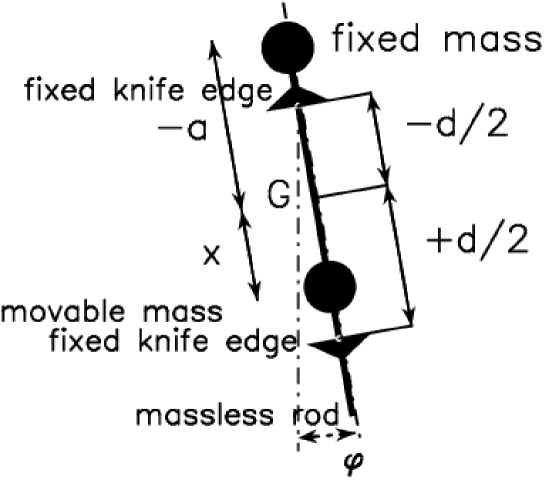
Fig. 1: Front view of idealized pendulum with two point masses and a massless rigid rod.

Then $d$ is the distance between the pivots, the center of mass is located at

• $\displaystyle\hskip 20.00003pt{b=\frac{-am_{f}+xm_{m}}{m_{f}+m_{m}}=\frac{x-a}{2}}$

and the moment of inertia about the center of mass at b is given by

• $\displaystyle\hskip 20.00003pt{I_{0}=\left(b+a\right)^{2}m_{f}+\left(b-x\right)^{2}m_{m}=\frac{m}{4}\left(x+a\right)^{2}}$

where $m=2m_{f}=2m_{m}$ is the total mass of the pendulum. The moment of inertia $I_{1}$ and $I_{2}$ with respect to the two pivots are

$$I_{1}=(\frac{a+x}{2})^{2}m+(\frac{d}{2}+b)^{2}m\quad,$$ (6)

and

$$I_{2}=(\frac{a+x}{2})^{2}m+(\frac{d}{2}-b)^{2}m\quad.$$ (7)

When $x$ determines a good mass configuration the resulting periods $T_{1}$ and $T_{2}$ of small oscillations about the two pivots, respectively, have equal values. Equation (1) gives

$$T_{1} = 2\pi\sqrt{\frac{m(b+\frac{d}{2})^{2}+\frac{m}{4}\left(x+a\right)^{2}}{mg\left|b+\frac{d}{2}\right|}}=2\pi\sqrt{\frac{\left(x-a+d\right)^{2}+\left(x+a\right)^{2}}{2g\left|x-a+d\right|}}$$

$$T_{2} = 2\pi\sqrt{\frac{m(b-\frac{d}{2})^{2}+\frac{m}{4}\left(x+a\right)^{2}}{mg\left|b-\frac{d}{2}\right|}}=2\pi\sqrt{\frac{\left(x-a-d\right)^{2}+\left(x+a\right)^{2}}{2g\left|x-a-d\right|}}$$

Then $T_{1}^{2}=T_{2}^{2}$ gives a cubic equation on the variable $x$. If it is assumed that

$$\left(x-a\right)^{2}-d^{2}<0$$ (8)

which occurs, for instance, when suspension points are the end points of the pendulum bar, one finds that

$$\left(x-a\right)\left[2\left(x^{2}+a^{2}\right)-d^{2}\right]=0$$ (9)

Its solutions are then given by

$$x = a,$$ (10)

$$x = \pm\sqrt{\frac{d^{2}}{2}-a^{2}}\,,$$ (11)

which represent all the possible positions of the movable weight giving a good mass configuration for the ideal Kater pendulum. The first solution, $x=a$, always exists. Furthermore, if $d/\sqrt{2}\geq a$ there are two additional positions which are symmetric with respect to the origin i.e. the middle point of the massless bar. Recall formula (2) to obtain the associated equivalent lengths. For the last two symmetric solutions it gives

• $\displaystyle\hskip 20.00003pt{l=d}$

But the equivalent length associated with the first solution is

$$l^{\prime}=\frac{d}{2}+2\frac{a^{2}}{d}$$ (12)

which in general does not coincide with the distance $d$ between the two pivots.

On the other hand if (8) is not assumed and we are in the more “pathological” case of a pendulum such that $\left(x-a\right)^{2}-d^{2}>0$ then $T_{1}^{2}=T_{2}^{2}$ reduces to a linear equation in the variable $x$ whose solution is

• $\displaystyle\hskip 20.00003pt{x=-\frac{d^{2}}{4a}}$

and the associated equivalent length is

• $\displaystyle\hskip 20.00003pt{l^{\prime\prime}=a+\frac{d^{2}}{4a}}$

which in general does not coincide with the distance $d$ between the two pivots.

Therefore for an ideal Kater pendulum the answers to the previous questions are:

1. there are at most three possible positions of the movable weight which determine a good mass configuration;

2. no; there always exists a good mass configuration whose associated equivalent length does not coincide with the distance between pivots.

An immediate consequence is that a parabolic fitting of the empirical data $\left(x,T\right)$ can’t be the best fitting since two parabolas never meet at three points! Moreover in some particular cases a parabolic fitting may cause strong distortions in determining good mass configurations. For example:

• if either $d/\sqrt{2}<a$ or (8) is not satisfied, the ideal Kater pendulum admits a unique good mass configuration; typically a parabolic fitting of data in this situation gives parabolas meeting only at imaginary points and the procedure stops;

• if $a\sim\pm d/2$ then the first solution of (9) is quite near to one of the two further symmetric solutions; a parabolic fitting of data gives only two intersection points but we do not know if one (and which one?) of them is nearer to the position associated with $l$ than to the one associated with $l^{\prime}$; in this situation also $l\sim l^{\prime}$ but they are not equal; then associating $l$ with a so determined good mass configuration may cause a relevant error in the final value of $g$.

One may object that we are discussing an empiric procedure by means of an ideal pendulum. In particular the position $x=a$ for the movable mass gives the completely symmetric mass configuration with respect to the middle point of the ideal pendulum bar. When a physical pendulum with $m_{f}\neq m_{m}$ is considered, what is such a mass configuration? Does it occur again?

The answer is “yes”. The key observation is that, for both pivots, the variable position $x$ of the movable mass and the resulting period $T$ of small oscillations are related by a cubic expressions of the following type (period-distance relations)

$$ax^{2}+bx+c=T^{2}+dxT^{2}\,,$$ (13)

where the coefficients $a,b,c,d$ depend on the pendulum parameters. This is precisely what Shedd and Birchby pointed out in their papers [2, 3, 4] giving theoretical and empirical evidences: they called the two (one for each pivot) equations (13) the equations of the reversible pendulum (see equations (10) and (11) of their first paper). Here we will refer to (13) as the cubic period–distance relation of the physical Kater pendulum considered. Note that only coefficients $a,b,c,d$ depend on the pendulum parameters, while the polynomial type of equation (13) does not depend on the choice of the pendulum. Thus, we can reduce the search for good mass configurations to a simple cubic equation similar to Eq. (9).

A first point in the present paper is to give a mathematically rigorous proof of the following

Theorem 1.1.

Let $p_{1}\left(x,y\right),p_{2}\left(x,y\right)$ be the following cubic polynomials

• $\displaystyle\hskip 20.00003pt{p_{i}\left(x,y\right)=A_{i}x^{2}+B_{i}x+C_{i}-y^{2}-D_{i}xy^{2}\quad,\quad i=1,2\ .}$

where $A_{i},B_{i},C_{i},D_{i}$ are real coefficients and $D_{1}\neq D_{2}$ . Then they admit always two real common roots and two pairs of complex conjugated common roots which may be real under suitable conditions on coefficients $A_{i},B_{i},C_{i},D_{i}$. Thinking them as points in the complex plane $\left(x,y\right)$ they are symmetric three by three with respect to the $x$–axis. Moreover these are all the common roots they can admit (that is: all the further common roots are “at infinity”).

This algebraic result leads to the following physical statement:

Corollary 1.2.

A physical Kater pendulum, with a “sufficiently long” bar, admits always a “good” mass configuration whose associated equivalent length does not in general coincide with the distance between the pivots.

Under “suitable conditions” on the pendulum parameters, it may admit two further “good” mass configurations. They correspond to symmetric positions of the movable mass, with respect to the middle point of the bar (if also the pivots are symmetrically located). They admit a common associated equivalent length which is precisely the distance between the pivots.

Moreover the pendulum can’t admit any further good mass configuration.

We will specify the meaning to the vague expressions “sufficiently long” and “suitable conditions”.

Although Shedd and Birchby knew in practice the content of the previous statement (they actually wrote down all the three good mass configurations in period–distance terms – see formulas (27) of their first paper) they couldn’t give a rigorous proof of it. They studied the geometry of the curves determined by the cubic period–distance relations by means of an old and non–standard “Newton’s classification”. They then arrived to conclude that (see the bottom lines of p. 281 in their first paper):

  

“Of the nine possible intersections of two cubic curves, in the present case three are imaginary or at infinity, three belong to the condition that $T$ is negative, and three belong to positive values of $T$, and can hence be experimentally realized.”

This conclusion does not exclude that, under some suitable conditions on the pendulum parameters, at least two of the three “imaginary or at infinity” intersections may become real and maybe physically realizable giving more than three good mass configurations. Actually we will see that these three intersections are not imaginary but definitely “at infinity” and they can never give physical results.

A second aim of the present paper is to observe that the best fitting of empirical data $\left(x,T\right)$ is then given by two cubic curves of type (13) instead of two parabolas of type (5). We will support this remark by experimental evidence for a real compound Kater pendulum.

The paper is organised as follows. Section 2 is devoted to prove Theorem 1.1. and the physical statement of Corollary 1.2.. Here we set the main notation and describe the physics of a real Kater pendulum. The proof of Theorem 1.1. is based on elementary elements of complex algebraic and projective geometry. Anyway a non–interested reader may skip it without losing any useful element to understand what follows. In Sec. 3 we describe an effective experiment. Section 4 is devoted to the analysis of experimental data by a linear fit of the period-distance cubics. An estimate of their intersection points gives the good mass configurations and the associated periods for our real Kater pendulum. Then the value of $g$. A comparison with a parabolic fitting of data is then given.

Appendix A is devoted to discuss the “suitable conditions” on the pendulum parameters under which the pendulum admits all the possible good mass configurations (see Corollary 1.2.). In Appendix B we collect some further numerical methods to analyse our empirical data.

2 Physics of the Kater reversible pendulum

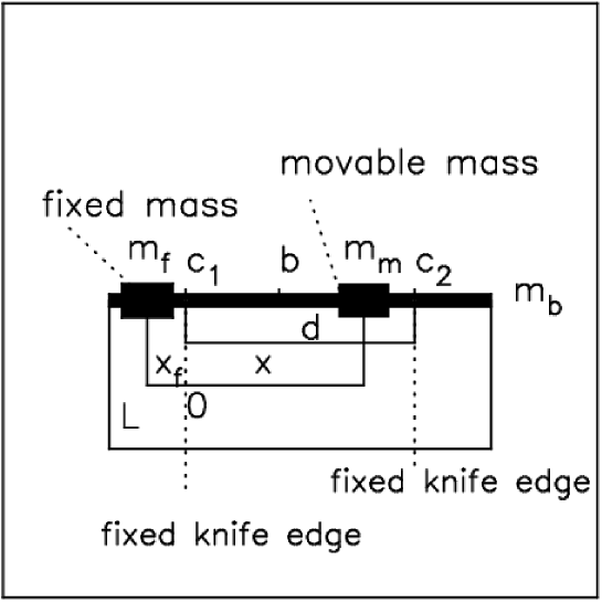
Fig. 2: Detailed side view of the Kater pendulum (not to scale).

Notation. Consider a physical Kater pendulum composed of a rigid bar equipped with two weights (see Fig. 2 and Fig. 3). The pendulum can be suspended by two knife–edges, $c_{1}$ and $c_{2}$, symmetrically located on the bar. The weight $m_{f}$ is placed in a fixed position which is not between the knives. The other one, $m_{m}$, can be moved along the bar. Small oscillations of the pendulum are parameterised by an angle $\varphi$ such that $\varphi\approx\sin\varphi$, that is, $\varphi^{3}\approx 0$. The equation of motion of the pendulum is then given by

$$\ddot{\varphi}+\frac{mgh_{i}}{I_{i}}\varphi=0\,,$$ (14)

where $g$ is the earth’s apparent gravitational acceleration, $m$ is the total mass of the pendulum, $h_{i}$ is the distance of the center of mass from the knife–edge $c_{i}$, and $I_{i}$ is the moment of inertia about $c_{i}$.

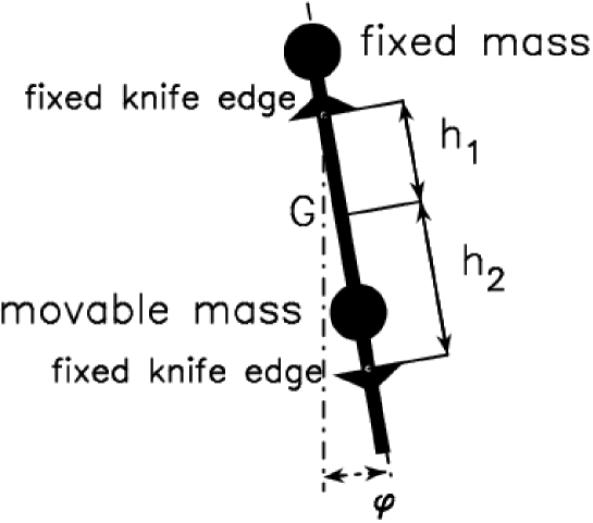
Fig. 3: Front view of the Kater pendulum (not to scale). The pendulum swings in the plane of the picture; its pivot can be inverted.

The Steiner’s theorem [6] asserts that

$$I_{i}=I_{0}+mh_{i}^{2}\,,$$ (15)

where $I_{0}$ is the moment of inertia with respect to the center of mass. The associated period of small oscillations is

$$T_{i}=\frac{2\pi}{{\omega}_{i}}=2\pi\sqrt{\frac{I_{i}}{mgh_{i}}}=2\pi\sqrt{\frac{I_{0}+mh_{i}^{2}}{mgh_{i}}}\,.$$ (16)

Equation (16) implies that the Kater pendulum oscillates with the same period as a simple pendulum whose length is given by

$$l_{i}=\frac{I_{i}}{mh_{i}}=\frac{I_{0}+mh_{i}^{2}}{mh_{i}}\,.$$ (17)

Assume now that the movable mass $m_{m}$ is placed at a point $x_{0}$ on the bar such that

$$T_{1}=T_{2}=T(x_{0})\,.$$ (18)

Such a point will be called a characteristic position of the pendulum. Equation (18) can be satisfied if and only if $l_{1}=l_{2}=l(x_{0})$. The length $l=l(x_{0})$ will be called the characteristic length of the pendulum associated with the characteristic position $x_{0}$. Analogously the associated periods $T(x_{0_{j}})$ will be the characteristic periods of the pendulum. The knowledge of $l(x_{0_{j}})$ and $T(x_{0_{j}})$ for each $j=1,2,3$ yields the value of $g$ from the relation

$$T=2\pi\sqrt{\frac{l}{g}}\,,$$ (19)

and therefore

$$g=\frac{4\pi^{2}}{T^{2}}\,.$$ (20)

The variable position of $m_{m}$ is described by a linear coordinate $x$ having origin at $c_{1}$. Then $c_{2}$ is the point $x=d>0$ (see Fig. 2) while the fixed weight is placed at $x_{f}$ such that $(d-L)/2<x_{f}<0$.

The movable and fixed weights are composed of disks whose radii are given respectively by $r_{m}$ and $r_{f}$.

$L$ is the length of the pendulum bar.

Therefore, the distance $h$ between the pendulum center of mass and the origin $c_{1}$ depends on the position $x$ of $m_{m}$ and is given by:

$$h=\frac{\frac{d}{2}m_{b}+x_{f}m_{f}+xm_{m}}{m_{b}+m_{f}+m_{m}}\,,$$ (21)

where $m_{b}$ is the mass of the bar. Set

$$m=m_{b}+m_{f}+m_{m}\,,$$ (22)

and

$$K=\frac{\frac{d}{2}m_{b}+x_{f}m_{f}}{m}\,.$$ (23)

Then $h$ can be rewrite as follows

$$h=K+\frac{m_{m}}{m}x\,.$$ (24)

The moment of inertia $I_{0}$ is then given by

$$I_{0}=\left(h-x_{f}\right)^{2}m_{f}+\left(h-x\right)^{2}m_{m}+\left(h-\frac{d}{2}\right)^{2}m_{b}+I_{0}^{\prime\prime}\,,$$ (25)

where

$$I_{0}^{\prime\prime}=\frac{r_{f}^{2}}{2}m_{f}+\frac{r_{m}^{2}}{2}m_{m}+\frac{L^{2}}{12}m_{b}\,.$$ (26)

Set

$$I_{0}^{\prime}=I_{0}^{\prime\prime}+m_{f}\left(x_{f}-K\right)^{2}+m_{b}\left(\frac{d}{2}-K\right)^{2}+m_{m}K^{2}\,,$$ (27)

and $I_{0}$ can be rewritten as follows:

$$I_{0}=m_{m}\frac{m-m_{m}}{m}x^{2}-2m_{m}Kx+I_{0}^{\prime}\,.$$ (28)

From Eq. (17) the condition (18) is satisfied if and only if

$$\frac{I_{0}+mh_{1}^{2}}{mh_{1}}=\frac{I_{0}+mh_{2}^{2}}{mh_{2}}\,,$$ (29)

which is equivalent to requiring that

$$\left(h_{1}-h_{2}\right)\left(mh_{1}h_{2}-I_{0}\right)=0\,.$$ (30)

From Eq. (24) we have

$$h_{1} = h=K+\frac{m_{m}}{m}x$$ (31)

$$h_{2} = d-h=d-K-\frac{m_{m}}{m}x\,,$$ (32)

and we get the first characteristic position by imposing that $h_{1}=h_{2}$, that is,

$$x_{0_{1}}=\frac{d}{2}+\frac{m_{f}}{2m_{m}}\left(d-2x_{f}\right)\,.$$ (33)

Two additional characteristic positions can be obtained by the second factor in Eq. (30). By letting $mh_{1}h_{2}-I_{0}=0$ and expressing $I_{0}$ as in Eq. (28), we have

$$x^{2}-dx-\frac{mK^{2}-mdK+I_{0}^{\prime}}{m_{m}}=0\,,$$ (34)

whose solutions are

$$x_{0_{2}} = \frac{d}{2}+\frac{1}{2}\sqrt{d^{2}+4\frac{mK^{2}-mdK+I_{0}^{\prime}}{m_{m}}}$$ (35)

$$x_{0_{3}} = \frac{d}{2}-\frac{1}{2}\sqrt{d^{2}+4\frac{mK^{2}-mdK+I_{0}^{\prime}}{m_{m}}}\,.$$ (36)

To determine the associated characteristic lengths $l(x_{0_{j}})$ use Eqs.  (17), (29), and (31). It follows that

$$l(x_{0_{j}})=\frac{I_{0}+m\left(K+\frac{m_{m}}{m}x_{0_{j}}\right)^{2}}{mK+m_{m}x_{0_{j}}}\,.$$ (37)

It is then easy to observe that $l(x_{0_{2}})$ and $l(x_{0_{3}})$ are equal and constant because $x_{0_{2}}$ and $x_{0_{3}}$ are symmetric. Precisely

$$l(x_{0_{2}})=l(x_{0_{3}})=h_{1}+h_{2}=d\,,$$ (38)

and they do not depend on the other physical parameters of the pendulum. On the contrary, this is not true for $l(x_{0_{1}})$ because

$$l(x_{0_{1}})=\frac{d}{2}+2\frac{I_{0}^{\prime\prime}}{md}+\frac{m_{f}\left(m_{m}+m_{f}\right)\left(d-2x_{f}\right)^{2}}{2m_{m}md}\,.$$ (39)

The reader may compare the characteristic positions (33), (35) and the associated characteristic lengths (39), (38), now obtained, with those given in Eq. (27) by Shedd and Birchby[2].

Moreover the period–distance relations of the pendulum (what Shedd and Birchby called “the equations of the Kater pendulum” [2]) can be obtained by Eq. (29) when $h_{1}$ and $h_{2}$ are expressed as in Eqs. (31). When the pendulum oscillates about the pivot $c_{i}$, the period $T_{i}$ and the distance $x$ results to be related by the following cubic relations

$$A_{i}x^{2}+B_{i}x+C_{i}=T_{i}^{2}+D_{i}xT_{i}^{2}\quad,\quad i=1,2\ ,$$ (40)

where

$$A_{1} = \frac{4\pi^{2}m_{m}}{gmK}$$ (41)

$$B_{1} = 0$$ (42)

$$C_{1} = \frac{4\pi^{2}}{gmK}\left(I_{0}^{\prime}+mK^{2}\right)$$ (43)

$$D_{1} = \frac{m_{m}}{mK}\,,$$ (44)

and

$$A_{2} = \frac{4\pi^{2}m_{m}}{gm(d-K)}$$ (45)

$$B_{2} = -\frac{8\pi^{2}m_{m}d}{gm\left(d-K\right)}$$ (46)

$$C_{2} = \frac{4\pi^{2}}{gm(d-K)}\left(I_{0}^{\prime}+m\left(d-K\right)^{2}\right)$$ (47)

$$D_{2} = -\frac{m_{m}}{m(d-K)}\,.$$ (48)

All the possible characteristic positions are then given by all the common roots of Eqs. (40).

Proof of Theorem 1.1.. For more details on the mathematics here involved see, for instance, Harris[7] or Shafarevich [8] among other introductory textbooks on algebraic geometry.

Consider $(x,y)$ as coordinates of points in the complex affine plane $\mathbf{C}^{2}$. Then equations $p_{1}\left(x,y\right)=0$ and $p_{2}\left(x,y\right)=0$ give two cubic complex algebraic curves, ${\mathcal{C}}_{1}$ and ${\mathcal{C}}_{2}$, whose intersection points are precisely the common roots of $p_{1}$ and $p_{2}$. We can compactify $\mathbf{C}^{2}$ by “adding a line at infinity”: this procedure produces the complex projective plane $\mathbf{P}_{\mathbf{C}}^{2}$. More precisely, we can consider our complex variables $x$ and $y$ to be a ratio of further variables, that is,

$$x=\frac{X}{Z}\ \quad{and}\quad y=\frac{Y}{Z}\,.$$ (49)

The equations defining ${\mathcal{C}}_{1}$ and ${\mathcal{C}}_{2}$ multiplied by $Z^{3}$ become the following

$$A_{1}X^{2}Z+B_{1}XZ^{2}+C_{1}Z^{3}=Y^{2}Z+D_{1}XY^{2}$$ (50)

$$A_{2}X^{2}Z+B_{2}XZ^{2}+C_{2}Z^{3}=Y^{2}Z+D_{2}XY^{2}\,.$$ (51)

which are the defining equations of the projective completions $\widetilde{{\mathcal{C}}}_{1}$ and $\widetilde{{\mathcal{C}}}_{2}$, respectively. The main ingredient of the present proof is the following

Theorem 2.1.

(Bezout) Given two distinct irreducible complex algebraic plane curves of degree $d_{1}$ and $d_{2}$, their projective completions admits a finite number of intersection points. Precisely if every intersection point is counted with its algebraic multiplicity then this number is $d_{1}d_{2}$.

In particular the projective completions $\widetilde{{\mathcal{C}}}_{1}$ and $\widetilde{{\mathcal{C}}}_{2}$ meet in 9 points, counted with their algebraic multiplicities. The Bezout theorem is a consequence of the Fundamental Theorem of Algebra which asserts that on the field $\mathbf{C}$ of complex numbers every polynomial admits as many roots as its degree.

The first step is to study the intersections “at infinity”, that is, which belong to the added “line at infinity.” The equation of this line is $Z=0$ and by Eq. (50) it intersects both our cubics at $y_{\infty}$ (that is, the point $X=Z=0$ which is the infinity point of the affine $y$-axis $x=0$) and in $x_{\infty}$ (that is, the point $Y=Z=0$ which is the infinity point of the affine $x$-axis $y=0$). Both of these are inflection points for ${\mathcal{C}}_{1}$ and ${\mathcal{C}}_{2}$. In $y_{\infty}$ the inflection tangent line of ${\mathcal{C}}_{1}$ is given by

• $\displaystyle\hskip 20.00003pt{t_{1}:D_{1}X+Z=0\,,}$

while the inflection tangent line of ${\mathcal{C}}_{2}$ is

• $\displaystyle\hskip 20.00003pt{t_{2}:D_{2}X+Z=0\,.}$

They cannot coincide since $D_{1}\neq D_{2}$. Therefore $y_{\infty}$ is a simple intersection point of our cubics, that is, it admits intersection multiplicity 1. On the other hand, in $x_{\infty}$ both ${\mathcal{C}}_{1}$ and ${\mathcal{C}}_{2}$ have the same inflection tangent line which is the infinity line $Z=0$. Then $x_{\infty}$ has intersection multiplicity 2. Consequently these infinity points count 3 of the 9 intersection points. The remaining 6 intersections must be affine, that is, they cannot belong to the compactifying line at infinity.

To find them note that for $i=1,2$

$$t_{i}\cap{\mathcal{C}}_{i}=y_{\infty}\,,$$ (52)

with intersection multiplicity 3 because it is an inflection point for ${\mathcal{C}}_{i}$ with tangent line $t_{i}$. On the other hand

$$t_{1}\cap{\mathcal{C}}_{2} = \{y_{\infty},P_{1},P_{2}\}$$ (53)

$$t_{2}\cap{\mathcal{C}}_{1} = \{y_{\infty},Q_{1},Q_{2}\}$$ (54)

where $P_{h}\not{=}y_{\infty}$, $Q_{k}\not{=}y_{\infty}$, and $P_{h}\not{=}Q_{k}$, because $t_{1}$ and $t_{2}$ are always distinct. Therefore, the affine intersection points of ${\mathcal{C}}_{1}$ and ${\mathcal{C}}_{2}$ cannot belong to the lines $t_{1}$ and $t_{2}$, and they can be recovered by studying the common solutions to the following equations

$$y^{2} = \frac{A_{1}x^{2}+B_{1}x+C_{1}}{1+D_{1}x}$$ (55)

$$y^{2} = \frac{A_{2}x^{2}+B_{2}x+C_{2}}{1+D_{2}x}\,,$$ (56)

because those points do not make the denominators vanish. So they are reduced to the roots of the following cubic equation

$$(A_{1}x^{2}+B_{1}x+C_{1})(1+D_{2}x)=(A_{2}x^{2}+B_{2}x+C_{2})(1+D_{1}x)\,.$$ (57)

It is a cubic equation with real coefficients. Therefore it admits 3 complex roots one of which is surely a real number. The remaining two roots are necessarily complex conjugated: their reality depends on the coefficients $A_{i},B_{i},C_{i},D_{i}$.

Proof of Corollary 1.2.. Recall the cubic period–distance relations (40). Setting $T_{1}=T_{2}=y$ they are represented by the two cubic curves ${\mathcal{C}}_{1}$ and $\mathcal{C}_{2}$ whose coefficients are assigned by formulas (41) and (45), respectively. Note that they are real numbers and $D_{1}\neq D_{2}$ since $d\neq 0$. The hypothesis of Theorem 1.1. are then satisfied and the characteristic positions of the pendulum must be represented by the real affine intersection points admitting $y\geq 0$. To conclude the proof observe that Eq. (57) divided out by $4\pi^{2}/gmK\left(d-K\right)$ gives exactly the cubic equation (30). The real root is then given by (33) and it always occurs when

• $\displaystyle\hskip 20.00003pt{\frac{m_{f}}{m_{m}}\left|d-2x_{f}\right|\leq L}$

The remaining two roots are then assigned by (35). A discussion of their reality is given in Appendix A.

3 The experiment

The physical parameters characterising our pendulum are given in Table 1; the digits in parentheses indicate the uncertainties in the last digit.

Table 1: The physical parameters characterising the pendulum.

$m_{m}$ (g)	$m_{f}$ (g)	$m_{b}$ (g)	$x_{f}$ (cm)	$l$ (cm)	$d$ (cm)	$r_{f}$ (cm)	$r_{m}$ (cm)
1399(1)	1006(1)	1249(1)	$-26.73(1)$	167.0(1)	99.3(1)	5.11(1)	5.12(1)

The bar length is measured by means of a ruler whose accuracy is $\pm 1$ mm. The radii $r_{m}$ and $r_{f}$ and the position $x_{f}$ are measured by a Vernier caliper accurate to $\pm 0.1$ mm. The masses $m_{b}$, $m_{m}$, and $m_{f}$ are determined by means of a precision balance accurate to one gram. With reference to the structural conditions in Appendix A, we are in the case 3.b i.e. all the three characteristic positions occurs and precisely $x_{0_{2}},x_{0_{3}}$ are placed between the knives while $x_{0_{1}}$ is on the opposite side of the bar with respect to $m_{f}$. By recalling Eqs.  (33) and (35), we expect that

$$x_{0_{1}} = (104.57\pm 0.11)\,{\mathrm{c}m}$$ (58)

$$x_{0_{2}} = (61.74\pm 0.40)\,{\mathrm{c}m}$$ (59)

$$x_{0_{3}} = (37.56\pm 0.31)\,{\mathrm{c}m}\,,$$ (60)

with associated characteristic lengths

$$l\left(x_{0_{1}}\right) = (121.44\pm 0.09)\,{\mathrm{c}m}$$ (61)

$$l\left(x_{0_{2}}\right)=l\left(x_{0_{3}}\right)=d = (99.3\pm 0.1)\,{\mathrm{c}m}\,.$$ (62)

Table 2: The experimental data.

$x$ (cm)	$T_{1}$ (s)	$T_{2}$ (s)
10	2.3613	2.0615
20	2.1492	2.0337
30	2.0363	2.0089
35	2.0016	1.9999
40	1.9838	1.9931
45	1.9733	1.9911
50	1.9754	1.9894
55	1.9799	1.9908
58	1.9846	1.9924
65	2.0055	2.0002
68	2.0173	2.0064
75	2.0470	2.0273
85	2.0939	2.0678
90	2.1224	2.0969
92	2.1334	2.1071
106	2.2178	2.2174
110	2.2441	2.2589
120	2.3078	2.3776

Throughout the experiment the movable mass $m_{m}$ will be placed in successive positions, generally 10 cm from each other, except near the theoretical characteristic positions (58) where the distances decrease (see the second column in Table 2)  . The period of small oscillation about the two pivots are measured for all those positions of $m_{m}$. These periods are measured by recording the time of each of 9 consecutive oscillations when the pendulum starts from the angle $\varphi_{0}\sim 6^{\circ}\pm 1^{\circ}$. For this purpose we used a photogate timed by an electronic digital counter  . We repeated the procedure for 18 positions of $m_{m}$, at first with respect to $c_{1}$ and then $c_{2}$. The average of the 9 values is taken to be the period at the given position of $m_{m}$ whose error is given by half of its maximum excursion, that is, $\approx~{}0.0018\,s$. The initial angle $\varphi_{0}$ is sufficiently small that an equation similar to Eq.  (14) is valid. By expanding an elliptic integral in a power series, it is possible to approximately express the period associated with the exact equation of pendulum motion

$$\ddot{\varphi}+\frac{mgh_{i}}{I_{i}}\sin\varphi=0$$ (63)

by adding corrective terms,[9, 6] to the period expression given in Eq. (19). In the next section we will evaluate such a correction. The results are reported in Table 2.

4 The linear fitting procedure

We now describe a linear fitting procedure used to fit the experimental data listed in Table 2  and empirically determine the characteristic positions. The numerical computations were obtained using MAPLE and some FORTRAN code  . From a numerical point of view we should fit the data by cubic polynomials like those in Eq. (40). Such a fitting can be treated linearly because the coefficients $D_{1}$ and $D_{2}$ may be determined a priori by Eqs. (41) and (45) which involve only the known physical parameters listed in Table 1. We obtain

$$D_{1} = (3.983\pm 0.01)\ 10^{-2}\,{\mathrm{c}m}^{-1}$$ (64)

$$D_{2} = (-4.2689\pm 0.0047)\ 10^{-3}\,{\mathrm{c}m}^{-1}\,.$$ (65)

We can obtain the desired fitting of the data obtained in Sec. 3 by applying the least squares method to the following function

$$\Xi_{i}\left(A_{i},B_{i},C_{i}\right)=\sum_{h=1}^{18}\left(\frac{T_{h,i}^{2}-\frac{A_{i}x_{h}^{2}+B_{i}x_{h}+C_{i}}{1+D_{i}x_{h}}}{2T_{h,i}\sigma_{T}}\right)^{2}\,,$$ (66)

where $(x_{h},T_{h,i})$ are the data of the $i$th set in Table 2  .

Two sources of error with period measurements were considered

• In any position and for both pivots, we considered the standard deviation of the 9 period electronic measurements, varying from 0.0003 s to 0.0036 s .

• The systematic error that formula 71 introduces on the data. For example when T=2.3 s (the maximum period here analysed) and $\varphi_{0}\sim 12^{\circ}$ the shift introduced on T is 0.006 s .

After this analysis we considered $\sigma_{T}=0.006$ s as estimated error for period measurements.

The obtained results are reported in Table 3 , Table 4 and visualised in Fig.4.

Table 3: Coefficients of the cubic curve ${\mathcal{C}}_{1}$ estimated by the linear method.

$A_{1}$	$(0.001607\pm 0.000003)\,s^{2}\,cm^{-2}$
$B_{1}$	$0\,\,s^{2}\,cm^{-1}$
$C_{1}$	$(7.641\pm 0.011)\,s^{2}$

Table 4: Coefficients of the cubic curve ${\mathcal{C}}_{2}$ estimated by the linear method.

$A_{2}$	($0.000172\pm 0.000002$)$\,s^{2}\,cm^{-2}$
$B_{2}$	($-0.03422\pm 0.00031$ )$\,s^{2}\,cm^{-1}$
$C_{2}$	($4.393\pm 0.01$) $\,s^{2}$

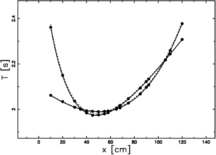
Fig. 4: Theoretical cubics (dotted line), fitted cubics (full line). and experimental data (filled points). The experimental errors are much smaller than the filled points drawn, so they are not visible within this plot.

The merit function $\chi^{2}$ and the associated $p$–values are reported in Table 5 and each of them have to be understood as the maximum probability to obtain a better fitting.

Table 5: $\chi^{2}$ and critical $p$–values for linear fitting by cubic curves

• $\displaystyle\hskip 20.00003pt{\begin{array}[]{ccc}\hline\cr\hline\cr{}{}{}{}\hfil&{\mathcal{C}}_{1},~{}degrees~{}of~{}freedom=16&;{\mathcal{C}}_{2}~{}degrees~{}~{}of~{}freedom=15\\ \hline\cr\vskip 3.0pt plus 1.0pt minus 1.0pt\cr\chi^{2}&2.69&1.57\\ \vskip 3.0pt plus 1.0pt minus 1.0pt\cr\int_{0}^{\chi^{2}}\chi^{2}(x,15)dx&0.00008&0.000005\\ \vskip 3.0pt plus 1.0pt minus 1.0pt\cr\vskip 3.0pt plus 1.0pt minus 1.0pt\cr\hline\cr\hline\cr\end{array}}$

The estimated cubic coefficients of Table 3 and Table 4 allow us to evaluate the characteristic positions and the associated characteristic periods by intersecting their upper branches We obtain a cubic equation whose numerical solutions are reported in Table 6.

Table 6: Estimated intersection points of fitting cubic curves.

$(x_{0_{1}},T(x_{0_{1}}))$	(106.015 cm, 2.2184 s)
$(x_{0_{2}},T(x_{0_{2}}))$	(62.541 cm, 1.9973 s)
$(x_{0_{3}},T(x_{0_{3}}))$	(35.779 cm, 1.9998 s)

Refer to Eqs. (20) and (61) to compute the associated values of $g$. We have

$$g_{1}=4\pi^{2}\frac{l(x_{0_{1}})}{T(x_{0_{1}})^{2}}$$ (67)

$$g_{2}=4\pi^{2}\frac{l(x_{0_{2}})}{T(x_{0_{2}})^{2}}$$ (68)

$$g_{3}=4\pi^{2}\frac{l(x_{0_{3}})}{T(x_{0_{3}})^{2}}\,,$$ (69)

and their numerical values are listed in Table 7.

Table 7: Values of $g$ obtained by formulas (67) and (70).

$g_{1}$	($974.15\pm 2.72$)  cm s-2
$g_{2}$	($982.65\pm 3.11$)  cm s-2
$g_{3}$	($980.20\pm 3.1$)  cm s-2
$\overline{g}$	($979.00\pm 1.72$)  cm s-2

Their average gives

$$\overline{g}=(979.00\pm 1.72)\,\mathrm{cm\,s}^{-2}\,.$$ (70)

where the uncertainty is found implementing the error propagation equation (often called law of errors of Gauss) when the covariant terms are neglected (see equation (3.14) in [11]). We now consider the correction arising from the approximation of the exact equation of pendulum motion (63) already mentioned at the end of the previous section. This correction gives:[9, 6]

$$T=2\,\pi\,\sqrt{{\frac{l}{g}}}\left(1+1/16\,{{\mathit{\varphi}_{0}}}^{2}\right)\quad,$$ (71)

and

$$g=4\pi^{2}{\frac{l}{{T^{2}}}}\left(1+1/16\,{{\mathit{\varphi}_{0}}}^{2}\right)^{2}\,.$$ (72)

A small increase in the value of $g$ is evident from Eq. (72), and we will refer to it as the finite amplitude correction (f.a.c.).

With the data listed in (7) we obtain

$$\overline{g}_{+}=(980.34\pm 1.74)\,\mathrm{cm\,s}^{-2}\,,$$ (73)

which is the gravity acceleration increased by the f.a.c.. An accurate measure of the value of $g$ in Turin[10] gives

$$g_{T}=980.534099(4)\,\mathrm{cm\,s}^{-2}\,.$$ (74)

This value will be considered as the “true value” of the acceleration due to the earth’s apparent gravity field in Turin   . By comparing it with $\overline{g}_{+}$, we see that our measurement is $-191$ ppm smaller than the ”true value.”

Note that the considered Kater pendulum admits characteristic positions sufficiently distant from each other (see formulas (58) and data collected in Table 6). Then it can be considered sufficiently “well–assembled”, which means that a parabolic fitting (of type (5)), of the empirical data $(x_{h},T_{h,i})$ collected in Table 2, should give a sufficiently precise evaluation of characteristic positions $x_{0_{2}},x_{0_{3}}$. As before we apply the least square method to the following function , but the sum is now extended to the first 13 entries of Table 2 in order to exclude the first intersection

$$\Theta_{i}\left(A_{i},B_{i},C_{i}\right)=\sum_{h=1}^{13}\left(\frac{T_{h,i}-\left(A_{i}x_{h}^{2}+B_{i}x_{h}+C_{i}\right)}{\sigma_{T}}\right)^{2}\,.$$ (75)

The coefficients of the fitting parabolas are reported in Tables( 8) and ( 9) ; the $\chi^{2}$ and the associated $p$–values are reported in Table 10 , in comparison the parabolic fit gives very bad results. .

Table 8: Coefficients of the first fitting parabola ${\mathcal{P}}_{1}$.

• $\displaystyle\hskip 20.00003pt{\begin{array}[]{cc}\hline\cr\hline\cr\vskip 3.0pt plus 1.0pt minus 1.0pt\cr A_{1}&(0.000180\pm 0.000002)\,s~{}cm^{-2}\\ \vskip 3.0pt plus 1.0pt minus 1.0pt\cr B_{1}&(-0.01959\pm 0.00017)\,s~{}cm^{-1}\\ \vskip 3.0pt plus 1.0pt minus 1.0pt\cr C_{1}&(2.494\pm 0.003)\,s\\ \vskip 3.0pt plus 1.0pt minus 1.0pt\cr\vskip 3.0pt plus 1.0pt minus 1.0pt\cr\hline\cr\hline\cr\end{array}}$

Table 9: Coefficients of the second fitting parabola ${\mathcal{P}}_{2}$.

• $\displaystyle\hskip 20.00003pt{\begin{array}[]{cc}\hline\cr\hline\cr\vskip 3.0pt plus 1.0pt minus 1.0pt\cr A_{2}&(0.000054\pm 0.000002)\,s~{}cm^{-2}\\ \vskip 3.0pt plus 1.0pt minus 1.0pt\cr B_{2}&(-0.00517\pm 0.00017)\,s~{}cm^{-1}\\ \vskip 3.0pt plus 1.0pt minus 1.0pt\cr C_{2}&(2.113\pm 0.004)\,s\\ \vskip 3.0pt plus 1.0pt minus 1.0pt\cr\vskip 3.0pt plus 1.0pt minus 1.0pt\cr\hline\cr\hline\cr\end{array}}$

Table 10: $\chi^{2}$ and critical $p$–values for linear fitting by parabolas ,
first 13 data , degrees of freedom =10

• $\displaystyle\hskip 20.00003pt{\begin{array}[]{ccc}\hline\cr\hline\cr{}{}{}{}\hfil&{\mathcal{P}}_{1}&{\mathcal{P}}_{2}\\ \hline\cr\vskip 3.0pt plus 1.0pt minus 1.0pt\cr\chi^{2}&893&12.5\\ \vskip 3.0pt plus 1.0pt minus 1.0pt\cr\int_{0}^{\chi^{2}}\chi^{2}(x,15)dx&1&0.74\\ \vskip 3.0pt plus 1.0pt minus 1.0pt\cr\vskip 3.0pt plus 1.0pt minus 1.0pt\cr\hline\cr\hline\cr\end{array}}$

Their intersection points are given in Table ( 11).

Table 11: Estimated intersection points of fitting parabolas.

• $\displaystyle\hskip 20.00003pt{\begin{array}[]{cc}\hline\cr\hline\cr\vskip 3.0pt plus 1.0pt minus 1.0pt\cr(x_{0_{2}},T(x_{0_{2}}))&(72.296cm:2.0207s)\\ \vskip 3.0pt plus 1.0pt minus 1.0pt\cr(x_{0_{3}},T(x_{0_{3}}))&(41.709cm:1.9908s)\\ \vskip 3.0pt plus 1.0pt minus 1.0pt\cr\vskip 3.0pt plus 1.0pt minus 1.0pt\cr\hline\cr\hline\cr\end{array}}$

We get then the following two evaluations of $g$:

$$g^{\prime}=4\pi^{2}\frac{d}{T(x_{0_{2}})^{2}}=(960.08\pm 3.00)\,\mathrm{cm\,s}^{-2}\,$$ (76)

$$g^{\prime\prime}=4\pi^{2}\frac{d}{T(x_{0_{3}})^{2}}=(989.11\pm 3.14)\,\mathrm{cm\,s}^{-2}\,\,.$$ (77)

Their average gives

$$\overline{g}_{parabolic}=(974.60\pm 2.18)\,\mathrm{cm\,s}^{-2}\,.$$ (78)

A comparison with $\overline{g}$ in (70) and $g_{T}$ in (74), gives a clear evidence of the better efficiency of a cubic fit with respect to a parabolic one.

5 Conclusions

We summarise the main results of our theoretical and numerical analysis

1. The three solutions of the Kater pendulum concerning the distance–period relationship discovered in 1907 by Shedd and Birchby in 1907 [2, 3, 4] are classified in a modern context

2. The first solution of the distance–period relationship allows to deduce a new formula of $g$ via the second equivalent length both in the idealized pendulum and in a commercial Kater pendulum, see respectively formula(12) and (39)

3. One of the main targets of our work ”the evaluation of g” gives oscillating results

   • : our best numerical fit to $T^{2}$ produces (the linear fit + non–linear correction) a value of g that is 191 ppm smaller than the ”true vale”

   • : our worst fit to $T^{2}$ (the non–linear fit + non–linear correction) gives a value of g that is 1978 ppm smaller than the ”true vale”

4. Concerning the fit to $T$ through a parabola we obtain high values of $\chi^{2}$ ($\chi^{2}$=893 for $C_{1}$ and $\chi^{2}$=12.51 for $C_{2}$) with respect to the linear fit to $T^{2}$ ($\chi^{2}$=2.69 for $C_{1}$ and $\chi^{2}$=1.57 for $C_{2}$). These high values of $\chi^{2}$ allow to rule out the physical significance of this type of fit.

A Reality of characteristic positions and structural conditions

The characteristic positions of our pendulum are given by Eqs. (33) and (35). The former, $x_{0_{1}}$, is always real. On the other hand $x_{0_{2}}$ and $x_{0_{3}}$ are real if and only if the square roots in Eq. (35) are real i.e.e if and only if

$$m_{m}d^{2}+4mdK-4mK^{2}-4I_{0}^{\prime}\geq 0\Longleftrightarrow$$ (A.1)

$$x_{f}^{2}-dx_{f}-\frac{(m_{m}+m_{b})d^{2}-4I_{0}^{\prime\prime}}{4m_{f}}\leq 0\,.$$ (A.2)

The latter are the “suitable conditions” on the pendulum parameters of Corollary 1.2..

To avoid the overlapping of $m_{f}$ with $c_{1}$ we have to impose that $x_{f}\leq-r_{f}$. Then Eq. (A.2) is equivalent to requiring that

$$md^{2}-4I_{0}^{\prime\prime}\geq 0\ \mathrm{and}\ \frac{d}{2}-\frac{1}{2}\sqrt{\frac{md^{2}-4I_{0}^{\prime\prime}}{m_{f}}}\leq x_{f}\leq-r_{f}\,.$$ (A.3)

Note that the condition on the right in Eq. (A.3) is not empty if

$$\frac{d}{2}-\frac{1}{2}\sqrt{\frac{md^{2}-4I_{0}^{\prime\prime}}{m_{f}}}\leq-r_{f}\Longleftrightarrow$$ (A.4)

$$d\geq 2\left(\frac{m_{f}r_{f}}{m_{b}+m_{m}}+\sqrt{\left(\frac{m_{f}r_{f}}{m_{b}+m_{m}}\right)^{2}+\frac{m_{f}r_{f}^{2}+I_{0}^{\prime\prime}}{m_{b}+m_{m}}}\right).$$ (A.5)

In particular, the latter ensures that the left condition in Eq. (A.3) is also satisfied because

$$md^{2}-4I_{0}^{\prime\prime}\geq 0\Longleftrightarrow d\geq 2\sqrt{\frac{I_{0}^{\prime\prime}}{m}}\,.$$ (A.6)

To avoid the overlapping of $m_{m}$ with the knife–edges it follows that either $r_{m}\leq x\leq d-r_{m}$ or $d+r_{m}\leq x\leq\frac{L+d}{2}$. After some algebra we get the following results.

Assume that $m_{m}>m_{f}$ and set

$$M_{1} = 2\frac{m_{m}r_{m}+m_{f}r_{f}}{m_{m}-m_{f}}$$ (A.7)

$$M_{2} = 2\left(\frac{m_{f}r_{f}}{m_{b}+m_{m}}+\sqrt{\left(\frac{m_{f}r_{f}}{m_{b}+m_{m}}\right)^{2}+\frac{m_{f}r_{f}^{2}+I_{0}^{\prime\prime}}{m_{b}+m_{m}}}\right)$$ (A.8)

$$S_{1} = \frac{m_{f}-m_{m}}{2m_{f}}d+\frac{m_{m}}{m_{f}}r_{m}$$ (A.9)

$$S_{2} = \frac{d}{2}-\frac{1}{2}\sqrt{\frac{md^{2}-4I_{0}^{\prime\prime}}{m_{f}}}$$ (A.10)

$$S_{3} = \frac{d}{2}-\frac{1}{2}\sqrt{\frac{m_{f}d^{2}+m_{b}d^{2}+4m_{m}r_{m}d-4m_{m}r_{m}^{2}-4I_{0}^{\prime\prime}}{m_{f}}}\,,$$ (A.11)

Then we have the following possibilities:

(1) $d<\min(M_{1},M_{2})$: in this case the pendulum admits only one characteristic position given by $x_{0_{1}}$ because by Eqs. (A.3) and (A.5), $x_{0_{2}}$ and $x_{0_{3}}$ are not real; $x_{0_{1}}$ is not between the knives, but occurs on the opposite side of the bar with respect to $m_{f}$; the system is in an almost symmetrical mass configuration of the pendulum.

(2) For $\min(M_{1},M_{2})\leq d<\max(M_{1},M_{2})$, we have the following possibilities:

(2a) If $M_{1}<M_{2}$: we get only the characteristic position $x_{0_{1}}$ which is between the knives if and only if $S_{1}\leq x_{f}\leq-r_{f}$; otherwise, $x_{0_{1}}$ is placed like in (1).

(2b) If $M_{2}<M_{1}$, we get all the characteristic positions; $x_{0_{1}}$ is like in (1) and $x_{0_{2}},x_{0_{3}}$ occur between the knives if and only if $S_{2}\leq x_{f}\leq\min(S_{3},-r_{f})$.

(3) For $\max(M_{1},M_{2})\leq d$, the pendulum admits all the characteristic positions $x_{0_{1}},x_{0_{2}},x_{0_{3}}$ which are placed as follows:

(3a) Only $x_{0_{1}}$ is placed between the knives when either

$$S_{1}<S_{2}\ \mbox{and}\ S_{1}\leq x_{f}\leq S_{2}\,,$$ (A.12)

or

$$S_{3}<-r_{f}\ \mbox{and}\ \max\left(S_{1},S_{3}\right)<x_{f}\leq-r_{f}\,.$$ (A.13)

(In particular, if $S_{3}<S_{1}$, we can also assume the position $x_{f}=S_{1}$ for the fixed weight $m_{f}$.)

(3b) only $x_{0_{2}},x_{0_{3}}$ are placed between the knives when $S_{2}<S_{1}$ and $S_{2}\leq x_{f}<S_{1}$.

(3c) We obtain all the possible characteristic positions $x_{0_{1}},x_{0_{2}},x_{0_{3}}$ between the knives when

$$\max(S_{1},S_{2})\leq x_{f}\leq\min(S_{3},-r_{f})\,.$$ (A.14)

In the concrete case considered in the Section 3 we have

$$M_{1} = (62.61\pm 0.25)\,{\mathrm{c}m}$$ (A.15)

$$M_{2} = (70.87\pm 0.05)\,{\mathrm{c}m}$$ (A.16)

$$S_{1} = (-12.28\pm 0.08)\,{\mathrm{c}m}$$ (A.17)

$$S_{2} = (-28.049\pm 0.075)\,{\mathrm{c}m}$$ (A.18)

$$S_{3} = (-7.62\pm 0.06)\,{\mathrm{c}m}\,,$$ (A.19)

where the uncertainty is found by applying the law of errors of Gauss with the uncertainties listed in Table 1. Therefore we are in the case 3.b.

B Further numerical methods

We outline three additional numerical methods that may be applied to analyse experimental data. The final results obtained by means of each method are reported in Table B.1.

Table B.1: Average values $\overline{g}$ and corrected values $\overline{g}_{+}$ (by f.a.c.).

algorithm	$\overline{g}$	$\overline{g}_{+}$
linear fitting by parabolas	($974.6\pm 2.17$) $cm\,s^{-2}$	($975.93\pm 2.20$) $cm\,s^{-2}$
linear fitting by cubics	($979.00\pm 1.72$) $cm\,s^{-2}$	($980.34\pm 1.74$) $cm\,s^{-2}$
non-linear fit	($977.25\pm 1.71$) $cm\,s^{-2}$	($978.25\pm 1.74$) $cm\,s^{-2}$
Cramer interpolation	($980.06\pm 4.88$) $cm\,s^{-2}$	($981.40\pm 4.89$) $cm\,s^{-2}$
Spline interpolation	($979.52\pm 1.73$) $cm\,s^{-2}$	($980.86\pm 1.74$) $cm\,s^{-2}$

B.1 The non-linear method

In the fitting procedure of data reported in Table 2, all the coefficients $A_{i},B_{i},C_{i}$ and $D_{i}$ are considered as unknown parameters to be estimated. Therefore a fitting procedure performed by means of cubic polynomials like those in Eq. (40) is necessarily a non-linear one. We want to apply the least square method to minimise the following functions

$$X_{i}\left(A_{i},B_{i},C_{i},D_{i}\right)=\sum_{h=1}^{18}\left(T_{h,i}^{2}-{\frac{A_{i}x_{h}^{2}+B_{i}x_{h}+C_{i}}{1+D_{i}x_{h}}}\right),$$ (B.1)

which are non-linear in the unknown coefficients. The procedure is to apply the NAG-Mark14 subroutine E04FDF to find an unconstrained minimum of a sum of 18 nonlinear functions in 4 variables (see Ref. [13]).

The final value of $g$ is reported in the Table B.1.

B.2 The Cramer interpolation method

We present here a method that reduces our analysis in a local neighbourhood of the estimated characteristic positions where a cubic behaviour of the fitting curves is imposed.

From Eqs. (41), (45), and (64) we know that $D_{1}$ and $D_{2}$ are completely determined by the pendulum parameters. Moreover, from Eqs. (41) we know that $B_{1}=0$. So to recover the remaining coefficients of ${\mathcal{C}}_{1}$ and ${\mathcal{C}}_{2}$, we need to interpolate two points of the first set of data in Table 2 and three points of the second one respectively. We have to solve a $2\times 2$ and a $3\times 3$ linear system by applying the Cramer theorem (which is the most practical method for solving a linear system of equations). If we choose data points that are close to a characteristic position, then the nearest point in ${\mathcal{C}}_{1}\cap{\mathcal{C}}_{2}$ to the chosen data will give an empirical estimation of such a characteristic position and its associated period. An iterated application of this procedure will produce a distribution of periods and we may obtain $g$ from the mean value and its statistical error from the standard deviation (see the last line of Table B.2).

Table B.2: The Cramer interpolation method.

Cramer Method
Char.	Chosen data		Intersection		Char.	g
position	Series 1	Series 2	Position	Period	length
$x_{0_{1}}$	15;18	15;17;18	105.773  cm	t1,1= 2.217  s	121.44  cm	975.73  cm s-2
$x_{0_{1}}$	15;17	15;16;17	106.360  cm	t1,2= 2.221  s	121.44 cm	971.92  cm s-2
$x_{0_{1}}$	16;18	16;17;18	106.108  cm	t1,3= 2.218  s	121.44 cm	974.08  cm s-2
$x_{0_{1}}$	15;18	15;16;18	106.189  cm	t1,4= 2.219  s	121.44 cm	973.44  cm s-2
$x_{0_{2}}$	7; 9	7; 8; 9	62.789  cm	t2,1= 1.996  s	99.30 cm	983.77  cm s-2
$x_{0_{2}}$	8;10	8; 9;10	62.056  cm	t2,2= 1.996  s	99.30 cm	983.79  cm s-2
$x_{0_{2}}$	9;11	9;10;11	61.962  cm	t2,3= 1.996  s	99.30 cm	984.28  cm s-2
$x_{0_{2}}$	10;12	10;11;12	61.990  cm	t2,4= 1.996  s	99.30 cm	984.44  cm s-2
$x_{0_{3}}$	2; 4	2; 3; 4	35.477 cm	t3,1= 1.999  s	99.30 cm	980.87  cm s-2
$x_{0_{3}}$	3; 5	3; 4; 5	36.207 cm	t3,2= 1.998  s	99.30 cm	981.97  cm s-2
$x_{0_{3}}$	4; 6	4; 5; 6	35.557 cm	t3,3= 1.999  s	99.30 cm	981.11  cm s-2
$x_{0_{3}}$	5; 7	5; 6; 7	36.668 cm	t3,4= 1.995  s	99.30 cm	985.38  cm s-2
$\overline{g}$=( 980.06 $\pm$ 4.89) cm s-2

The results obtained for every interpolation are reported in Table B.2; the chosen data points in the second and third columns are enumerated as they appear in Table 2.

B.3 Cubic Spline Interpolation

The last data analysis method to be proposed is the cubic spline interpolation (subroutine SPLINE and SPLINT from Numerical Recipes II). Once the three intersections are obtained, the procedure was similar to the linear/nonlinear case and the final value of $g$ is reported in Table B.1.

References

- [1] D. Randall Peters, “Student-friendly precision pendulum,” Phys. Teach., Vol. 37, (1999),pp 390–393.
- [2] J.C. Shedd , J.A. Birchby, “A study of the reversible pendulum. Part I. Theoretical considerations,” Phys. Rev. (Series I), Vol. 25 , (1907),pp 274–293
- [3] J.C. Shedd , J.A. Birchby, “A study of the reversible pendulum. Part II. Experimental verifications,” Phys. Rev. (Series I), Vol 34, (1912) , pp 110–124
- [4] J.C. Shedd , J.A. Birchby, “A study of the reversible pendulum. Part III. A critique of captain Kater’s paper of 1818,” Phys. Rev. 1 , Vol. 457, (1913), pp 457– 462
- [5] D. Candela, K. M. Martini, R. V. Krotkov, K. H. Langley, “Bessel’s improved Kater pendulum in the teaching lab,” Am. J. Phys. , Vol. 69, (2001, pp 714–720
- [6] R. Resnick, D. Halliday, K. S. Krane, Physics ,John Wiley & Sons, New York, 1991.
- [7] J. Harris, Algebraic Geometry , Springer-Verlag, New York, 1992.
- [8] I. R. Shafarevich, Basic Algebraic Geometry , Springer-Verlag, New York ,1977.
- [9] R. A. Nelson , M. G. Olsson, “The pendulum-rich physics from a simple system,” Am. J. Phys.,Vol. 54,(1986), pp 112–121 .
- [10] G. Cerutti , P. DeMaria, “Misure assolute dell’ accelerazione di gravità a Torino,” In: Technical Report R432, Istituto di Metrologia “G. Colonnetti” , Turin ,1996 .
- [11] Philip R. Bevington , D. Keith Robinson, Data Reduction and Error Analysis for the Physical Sciences, McGraw-Hill, Inc., New York, 1992.
- [12] P. Moreland, “Improving precision and accuracy in the g lab,” Phys. Teach., Vol. 38, 367–369 (2000).
- [13] NAG , http://www.nag.co.uk/
- [14] Numerical Recipes , http://www.nr.com/