Turbulent-laminar patterns in plane Couette flow

Abstract

Regular patterns of turbulent and laminar fluid motion arise in plane Couette flow near the lowest Reynolds number for which turbulence can be sustained. We study these patterns using an extension of the minimal flow unit approach to simulations of channel flows pioneered by Jiménez and Moin. In our case computational domains are of minimal size in only two directions. The third direction is taken to be large. Furthermore, the long direction can be tilted at any prescribed angle to the streamwise direction. We report on different patterned states observed as a function of Reynolds number, imposed tilt, and length of the long direction. We compare our findings to observations in large aspect-ratio experiments.

Published version appears as D. Barkley and L.S. Tuckerman, Turbulent-laminar patterns in plane Couette flow, in IUTAM Symposium on Laminar Turbulent Transition and Finite Amplitude Solutions, T. Mullin and R. Kerswell (eds), Springer, Dordrecht, pp. 107–127 (2005).

I INTRODUCTION

In this chapter we consider plane Couette flow – the flow between two infinite parallel plates moving in opposite directions. This flow is characterized by a single non-dimensional parameter, the Reynolds number, defined as $Re=hU/\nu$, where $2h$ is the gap between the plates, $U$ is the speed of the plates and $\nu$ is the kinematic viscosity of the fluid. See figure 1. For all values of $Re$, laminar Couette flow ${\bf u_{C}}\equiv y{\bf\hat{x}}$ is a solution of the incompressible Navier-Stokes equations satisfying no-slip boundary conditions at the moving plates. This solution is linearly stable at all values of $Re$. Nevertheless it is not unique. In particular, for $Re$ greater than approximately $325$ Dauchot and Daviaud (1995), turbulent states are found in experiments and numerical simulations. Our interest is in the flow states found as one decreases $Re$ from developed turbulent flows to the lowest limit for which turbulence exists.

Figure 1: Plane Couette geometry. Plates separated by a gap $2h$ move at speeds $\pm U$. The coordinate system we use is as shown, with $y=0$ corresponding to midgap.

Our work is motivated by the experimental studies of Prigent and coworkers (2001,2002,2003,2005) on flow in a very large aspect-ratio plane Couette apparatus. Near the minimum $Re$ for which turbulence is sustained, they find remarkable, essentially steady, spatially-periodic patterns of turbulent and laminar flow. These patterns emerge spontaneously from featureless turbulence as the Reynolds number is decreased. Figure 2 shows such a pattern from numerical computations presented in this chapter. Two very striking features of these patterns are their large wavelength, compared with the gap between the plates, and the fact that the patterns form at an angle to the streamwise direction.

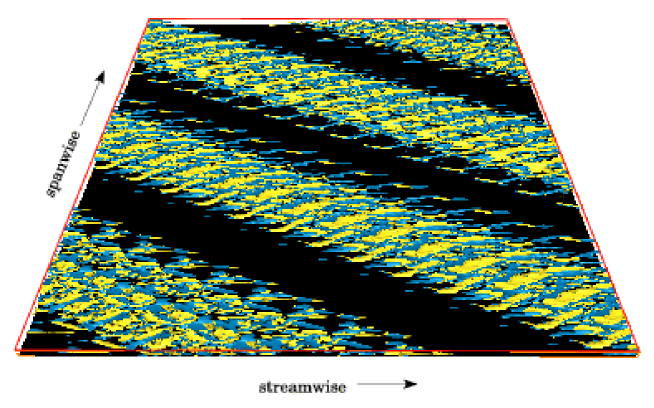
Figure 2: Turbulent-laminar pattern at Reynolds number 350. Isosurfaces of streamwise vorticity ($\omega=\pm 0.5$) are shown at one instant in time. For clarity the bottom plate is shown in black while the top plate is transparent. The streamwise and spanwise extent of the region shown are 60 times the plate separation $2h$.

Fluid flows exhibiting coexisting turbulent and laminar regions have a significant history in fluid dynamics. In the mid 1960s a state known as spiral turbulence was first discovered Coles (1965); van Atta (1966); Coles and van Atta (1966) in counter-rotating Taylor–Couette flow. This state consists of a turbulent and a laminar region, each with a spiral shape. The experiments of Prigent et al.  (2001,2002, 2003,2005) in a very large aspect-ratio Taylor–Couette system showed that in fact the turbulent and laminar regions form a periodic pattern, of which the original observations of Coles and van Atta comprised only one wavelength. Cros and Le Gal (2002) discovered large-scale turbulent spirals as well, in the shear flow between a stationary and a rotating disk. When converted to comparable quantities, the Reynolds-number thresholds, wavelengths, and angles are very similar for all of these turbulent patterned flows.

II METHODS

Our computational technique Barkley and Tuckerman (2005) extends the minimal flow unit methodology pioneered by Jiménez and Moin (1991) and by Hamilton et al. (1995) and so we begin by recalling this approach. Turbulence near transition in plane Couette and other channel flows is characterized by the cyclical generation and breakdown of streaks by streamwise-oriented vortices. The natural streak spacing in the spanwise direction is about 4–5$h$. In the minimal flow unit approach, the smallest laterally periodic domain is sought that can sustain this basic turbulent cycle. For plane Couette flow at $Re=400$, Hamilton et al. (1995) determined this to be approximately $(L_{x},L_{y},L_{z})=(4h,2h,6h)$. This domain is called the minimal flow unit (MFU). The fundamental role of the streaks and streamwise vortices is manifested by the fact that the spanwise length of the MFU is near the natural spanwise streak spacing. Figure 3(a) shows the MFU in streamwise-spanwise coordinates.

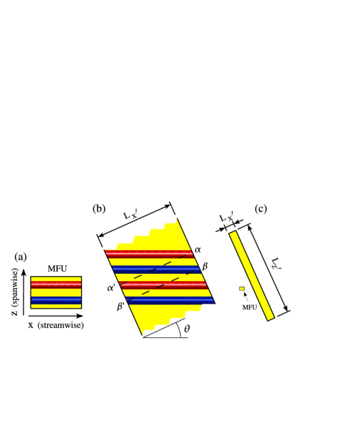
Figure 3: Simulation domains. The wall-normal direction $y$ is not seen; $L_{y}=2h$. The bars represent streamwise vortex pairs with a spanwise spacing of $4h$. (The vortices are schematic; these are dynamic features of the actual flow.) (a) MFU domain of size $6h\times 4h$. (b) Central portion of a domain [on the same scale as (a)] tilted to the streamwise direction. $\alpha$, $\alpha^{\prime}$ and $\beta$, $\beta^{\prime}$ are pairs of points identified under periodic boundary conditions in ${x^{\prime}}$. (c) Full tilted domain with $L_{x^{\prime}}=10h$, $L_{z^{\prime}}=120h$, $\theta=24^{\circ}$. On this scale the MFU domain, shown for comparison, is small.

We extend the MFU computations in two ways. First we tilt the simulation domain in the lateral plane at angle $\theta$ to the streamwise direction [Figure 3(b)]. We use ${x^{\prime}}$ and ${z^{\prime}}$ for the tilted coordinates. We impose periodic lateral boundary conditions on the tilted domain. To respect the spanwise streak spacing while imposing periodic boundary conditions in ${x^{\prime}}$, the domain satisfies $L_{x^{\prime}}\sin\theta\simeq 4h$ for $\theta>0$. (For $\theta=0$, we require $L_{x^{\prime}}\gtrsim 6h$.) Secondly, we greatly extend one of the dimensions, $L_{z^{\prime}}$, past the MFU requirement [Figure 3(c)], in practice between $30h$ and $220h$, usually $120h$.

This approach presents two important advantages, one numerical and the other physical. First, it greatly reduces the computational expense of simulating large length-scale turbulent-laminar flows. Our tilted domains need only be long perpendicular to the turbulent bands. In the direction in which the pattern is homogeneous, the domains are of minimal size, just large enough to capture the streamwise vortices typical of shear turbulence. Second, the approach allows us to impose or restrict the pattern orientation and wavelength. We can thereby investigate these features and establish minimal conditions necessary to produce these large-scale patterns.

We now present some further details of our simulations. We consider the incompressible Navier–Stokes equations written in the primed coordinate systems. After nondimensionalizing by the plate speed $U$ and the half gap $h$, these equations become

$$\frac{\partial{\bf u^{\prime}}}{\partial t}+({\bf u^{\prime}}\cdot\nabla^{\prime}){\bf u^{\prime}} = -\nabla^{\prime}p^{\prime}+\frac{1}{Re}\nabla^{\prime 2}{\bf u^{\prime}}\quad\hbox{in $\Omega$},$$ (1a)

$$\nabla^{\prime}\cdot{{\bf u^{\prime}}} = 0\quad\hbox{in $\Omega$},$$ (1b)

where ${\bf u^{\prime}}({\bf x^{\prime}},t)$ is the velocity field and $p^{\prime}({\bf x^{\prime}},t)$ is the static pressure in the primed coordinate system, and $\nabla^{\prime}$ is used to indicate that derivatives are taken with respect to primed coordinates. $\Omega$ is the computational domain. In these coordinates, the no-slip and periodic boundary conditions are

$${\bf u^{\prime}}(x^{\prime},y=\pm 1,z^{\prime}) = \pm(\cos\theta,0,\sin\theta)$$ (2a)

$${\bf u^{\prime}}(x^{\prime}+L_{x^{\prime}},y,z^{\prime}) = {\bf u^{\prime}}(x^{\prime},y,z^{\prime})$$ (2b)

$${\bf u^{\prime}}(x^{\prime},y,z^{\prime}+L_{z^{\prime}}) = {\bf u^{\prime}}(x^{\prime},y,z^{\prime})$$ (2c)

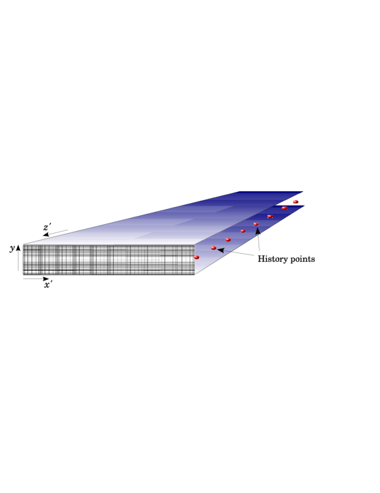
Figure 4: Simulation domain. The $({x^{\prime}},y)$ grid is the actual spectral-element mesh used for the case $L_{{x^{\prime}}}=10$. Only part of the ${z^{\prime}}$ direction is shown. In practice we use 32 history points in the ${z^{\prime}}$ direction.

The equations are simulated using the spectral-element (${x^{\prime}}$-$y$) – Fourier (${z^{\prime}}$) code Prism Henderson and Karniadakis (1995). We use a spatial resolution consistent with previous studies Hamilton et al. (1995); Waleffe (2003, 2005). Specifically, for a domain with dimensions $L_{x^{\prime}}$ and $L_{y}=2$, we use a computational grid with close to $L_{x^{\prime}}$ elements in the ${x^{\prime}}$ direction and 5 elements in the $y$ direction. Within each element, we usually use $6$th order polynomial expansions for the primitive variables. Figure 4 shows a spectral element mesh used for the case of $L_{x^{\prime}}=10$. In the ${z^{\prime}}$ direction, a Fourier representation is used and the code is parallelized over the Fourier modes. Our typical domain has $L_{z^{\prime}}=120$, which we discretize with 1024 Fourier modes or gridpoints. Thus the total spatial resolution we use for the $L_{x^{\prime}}\times L_{y}\times L_{z^{\prime}}=10\times 2\times 120$ domain can be expressed as $N_{x^{\prime}}\times N_{y}\times N_{z^{\prime}}=61\times 31\times 1024$.

We shall always use $(x,y,z)$ for the original streamwise, cross-channel, spanwise coordinates (Figure 1). We obtain usual streamwise, and spanwise components of velocity and vorticity using $u=u^{\prime}\cos\theta+w^{\prime}\sin\theta$ and $w=u^{\prime}\sin\theta-w^{\prime}\cos\theta$, and similarly for vorticity. The kinetic energy reported is the difference between the velocity ${\bf u}$ and simple Couette flow ${\bf u_{C}}$, i.e. $E=\frac{1}{2}((u-u_{C})^{2}+v^{2}+w^{2})$.

We have verified the accuracy of our simulations in small domains by comparing to prior simulations Hamilton et al. (1995). In large domains we have examined mean velocities, Reynolds stresses, and correlations in a turbulent-laminar flow at $Re=350$ and find that these reproduce experimental results from Taylor–Couette Coles and van Atta (1966) and plane Couette Hegseth (1996) flow. While neither experimental study corresponds exactly to our case, the agreement supports our claim that our simulations correctly capture turbulent-laminar states.

The procedure we use to initiate turbulence is inspired by previous investigations of plane Couette flow in a perturbed geometry. We recall that laminar plane Couette flow is linearly stable at all Reynolds numbers. It has been found, experimentally Bottin et al. (1998) and numerically Barkley and Tuckerman (1999); Tuckerman and Barkley (2002), that the presence of a wire Bottin et al. (1998) or a ribbon Barkley and Tuckerman (1999); Tuckerman and Barkley (2002) oriented along the spanwise direction causes the flow in the resulting geometry to become linearly unstable to either a steady or a turbulent state containing streamwise vortices. We simulate such a flow with a ribbon which is infinitesimal in the ${x^{\prime}}$ direction, occupies 30% of the cross-channel direction $y$ and spans the entire ${z^{\prime}}$ direction. At $Re=500$, the effect of such a ribbon is to produce a turbulent flow quickly without the need to try different initial conditions. Once the turbulent flow produced by the ribbon is simulated for a few hundred time units, the ribbon can be removed and the turbulence remains. This procedure is used to initialize turbulent states for the simulations to be described below.

III APPEARANCE OF TURBULENT-LAMINAR BANDS

III.1 Basic phenomenon

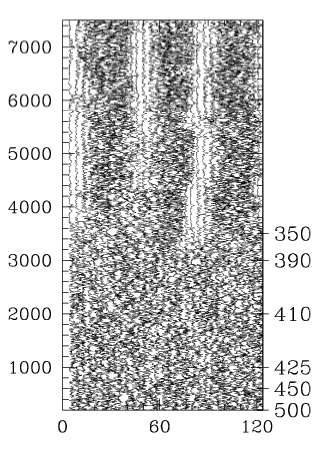
Figure 5: Space-time diagram. Kinetic energy $E({x^{\prime}}=0,y=0,{z^{\prime}})$ at 32 equally spaced points in ${z^{\prime}}$ in a domain with $L_{x^{\prime}}\times L_{y}\times L_{z^{\prime}}=10\times 2\times 120$ with tilt $\theta=24^{\circ}$. The Reynolds number is decremented in discrete steps (right). Three long-lasting and well-separated laminar regions emerge spontaneously from uniform turbulence as $Re$ is decreased.

We begin with one of our first simulations, in a domain tilted at angle $\theta=24^{\circ}$. This angle has been chosen to be close to that observed experimentally near pattern onset. The simulation shows the spontaneous formation of a turbulent-laminar pattern as the Reynolds number is decreased. We initiated a turbulent flow at $Re=500$ by perturbing laminar Couette flow with a ribbon as described in Section II. Time zero in Figure 5 corresponds to the removal of the ribbon. The flow is simulated for 500 time units at $Re=500$ and the kinetic energy $E$ is measured at 32 points equally spaced in ${z^{\prime}}$ along the line ${x^{\prime}}=y=0$ in the mid-channel shown in Figure 4. The corresponding 32 time series are plotted at the corresponding values of ${z^{\prime}}$. At $Re=500$, there is no persistent large-scale variation in the flow, a state which we describe as uniform turbulence. (This is not the homogeneous or fully developed turbulence that exists at higher Reynolds numbers or in domains without boundaries.) At the end of 500 time units, $Re$ is abruptly changed to $Re=450$ and the simulation continued for another 500 time units. Then $Re$ is abruptly lowered to $Re=425$ and the simulation is continued for 1000 time units, etc. as labeled on the right in Figure 5.

At $Re=350$ we clearly see the spontaneous formation of a pattern. Out of uniform turbulence emerge three regions of relatively laminar flow between three regions of turbulent flow. (We will later discuss the degree to which the flow is laminar.) While the individual time traces are irregular, the pattern is itself steady and has a clear wavelength of 40 in the ${z^{\prime}}$ direction. This Reynolds number and wavelength are very close to what is seen in the experiments.

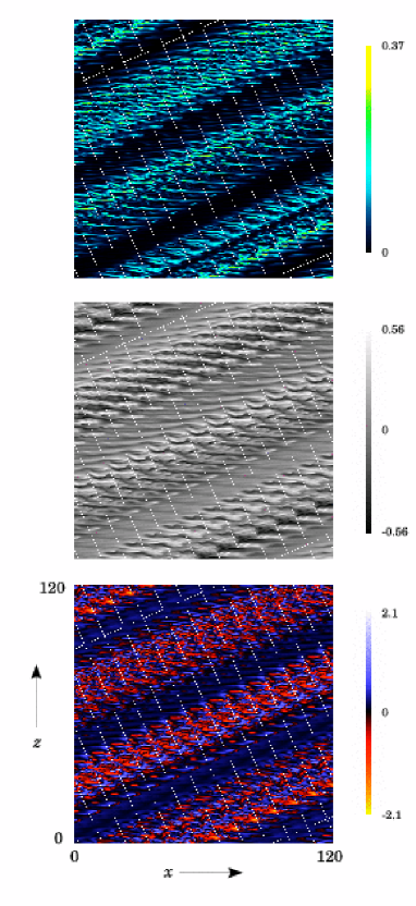
Figure 6: Turbulent-laminar pattern at $Re=350$. The kinetic energy, streamwise velocity, and streamwise vorticity are visualized in the $y=0$ plane, midway between and parallel to the moving plates. The computational domain (outlined in white, tilted at angle $\theta=24^{\circ}$) is repeated periodically to tile an extended region in $x$-$z$ coordinates. Streamwise streaks, with spanwise separation approximately $4h$, are visible at the edges of the turbulent regions.

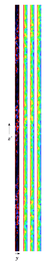
Figure 7: Turbulent-laminar pattern at $Re=350$ viewed between the moving plates (${x^{\prime}}=0$ plane). Left plot shows streamwise vorticity. The other three plots show contours of streamwise velocity at three times separated by 100 time units (time increasing left to right). The vorticity plot and the first velocity plot correspond to the field seen in Figure 7.

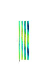
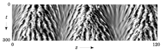
Figure 8: Mean and rms velocity fields for the turbulent-laminar pattern. From left to right: mean streamwise velocity, mean spanwise velocity, rms streamwise velocity and rms spanwise velocity. The rms velocities are maximal in the lightest regions. Only the central half ($30\leq{z^{\prime}}\leq 90$) of the computational domain is shown.

Figure 9: Space-time plot showing dynamics of the turbulent-laminar pattern. Streamwise velocity is sampled along a spanwise cut through the flow field (the line $x=y=0$ in the reconstructed flows in Figure 7). Time zero corresponds to the time of Figure 7. The streaks propagate away from the center of the turbulent regions toward the laminar regions.

III.2 Visualizations

Figure 7 shows visualizations of the flow at the final time in Figure 5. Shown are the kinetic energy, streamwise velocity, and streamwise vorticity in the midplane between the plates. The computational domain is repeated periodically to tile an extended region of the midplane. The angle of the pattern is dictated by the imposed tilt of the computational domain. The wavelength of the pattern is not imposed by the computations other than that it must be commensurate with $L_{z^{\prime}}120$. The vorticity isosurfaces of this flow field were shown in Figure 2. Spanwise and cross-channel velocity components show similar banded patterns.

Clearly visible in the center figure are streamwise streaks typical of shear flows. These streaks have a spanwise spacing on the scale of the plate separation but have quite long streamwise extent. We stress how these long streaks are realized in our computations. A streak seen in Figure 7 typically passes through several repetitions of the computational domain, as a consequence of the imposed periodic boundary conditions. In the single tilted rectangular computational domain, a single long streak is actually computed as several adjacent streaks connected via periodic boundary conditions.

Figure 7 shows the streamwise vorticity and velocity fields between the plates. The two leftmost images correspond to the same field as in Figure 7. The streamwise vorticity is well localized in the turbulent regions. Mushrooms of high- and low-speed fluid, corresponding to streamwise streaks, can be seen in the turbulent regions of flow. Dark velocity contours, corresponding to fluid velocity approximately equal to that of the lower and upper moving plates, are seen to reach into the center of the channel in the turbulent regions. In the center of the laminar regions, where the flow is relatively quiescent (Figure 5), there is very little streamwise vorticity and the streamwise velocity profile is not far from that of laminar Couette flow. In particular, no high- or low-speed fluid reaches into the center of the channel in these laminar regions.

In Figure 9 we show the mean and rms of the streamwise and spanwise velocity components obtained from averages over $T=2000$ time units. These results show that the mean flow is maximal at the boundaries separating the turbulent and laminar regions while the fluctuations are maximal in the middle of the turbulent bands. This agrees with the experimental observations of of Prigent et al.  (2001,2002, 2003,2005) Note further that the regions of high fluctuation have approximately the same rhombic shape as the turbulent regions shown by Coles and van Atta (1966) in experiments on Taylor–Couette flow. Finally, Figure 9 shows a space-time plot of streamwise velocity along the spanwise line $x=y=0$. Specifically, data is taken from reconstructed flows as in Figure 7. Time zero in Figure 9 corresponds to the field in Figure 7. Time is taken downward in this figure to allow for comparison with a similar figure from the experimental study by Hegseth (1996: figure 6) showing the propagation of streaks away from the center of turbulent regions. Our results agree quantitatively with those of Hegseth. We find propagation of streaks away from the center of the turbulent regions with an average spanwise propagation speed of approximately 0.054 in units of the plate speed $U$. Translating from the diffusive time units used by Hegseth, we estimate the average spanwise propagation speed of streaks in his data to be approximately 0.060 at Reynolds number $420$. This space-time plot again shows the extent to which there is some small activity in the regions we refer to as laminar.

III.3 Average spectral coefficients

Figure 10: Evolution of $\langle|\hat{w}_{m}|\rangle$, which is an average over time $T$ of the modulus of the Fourier transform in the ${z^{\prime}}$ direction of 32 spanwise velocity samples taken along the line $({x^{\prime}}=0,y=0)$. The components with wavenumber $m=3$ (solid curve), $m=2$ (long-dashed curve), $m=1$ (short-dashed curve) and $m=0$ (dotted curve) can be used as a quantitative diagnostic of a turbulent-laminar pattern. For example, the dominance of the $m=3$ component indicates a pattern containing three turbulent bands. From left to right, the average is taken over $T=10$, $T=30$, $T=100$, $T=300$, and $T=1000$.

We have determined a good quantitative diagnostic of the spatial periodicity of a turbulent-laminar pattern. We use the same data as that presented in Figure 5, i.e. velocities at 32 points along the line ${x^{\prime}}=y=0$ in the midplane along the long direction, at each interval of $100$ time steps: $100\Delta t=1$. We take a Fourier transform in ${z^{\prime}}$ of the spanwise velocity $w$, yielding $\hat{w}_{m}$. We take the modulus $|\hat{w}_{m}|$ to eliminate the spatial phase. Finally, we average over a time $T$ to obtain $\langle|\hat{w}_{m}|\rangle$. Figure 10 shows the evolution of $\langle|\hat{w}_{m}|\rangle$ for wavenumbers $m=3$, $m=2$, $m=1$, and $m=0$ during one of our simulations (shown below in Figure 11, which is a continuation of that shown in Figure 5). As before, the vertical axis corresponds to time, and also to Reynolds number, which was decreased in steps of $\Delta Re=10$. We average successively over $T=10$, $T=30$, $T=100$, $T=300$, and $T=1000$ and observe the short-term fluctuations gradually disappear, leaving the long-term features which will be discussed in the next section. We have chosen $T=500$ as the best compromise between smoothing and preserving the detailed evolution.

IV DEPENDENCE ON REYNOLDS NUMBER

We have investigated in detail the Reynolds-number dependence of the $\theta=24^{\circ}$ case. To this end, we have carried out two simulations, shown in Figure 11. In each the Reynolds number is lowered at discrete intervals in time, but following a different sequence in the two cases. For each case, we present a space-time diagram of $E({x^{\prime}}=0,y=0,{z^{\prime}},t)$ at 32 values of ${z^{\prime}}$. The Reynolds-number sequence is shown on the right of each diagram and the time (up to $T=59,000$) on the left. Each space-time diagram is accompanied by a plot showing the evolution of its average spectral coefficients, as defined above.

Figure 11: Two time series at $\theta=24^{\circ}$. The Reynolds number is lowered in steps, but at different instants to generate the two evolutions shown. For each case, we show $w$ at 32 points along the ${z^{\prime}}$ direction on the right and the spectral components $\langle|\hat{w}_{m}|\rangle$ on the left. Left: uniform turbulence is succeeded by the formation of three bands, then two, then a single band (a localized state) and finally by laminar Couette flow. Right: two bands disappear almost simultaneously at $Re=320$. The remaining band moves toward the left, periodically emitting turbulent spurs, of which one finally becomes a second turbulent band.

Careful observation of Figure 5 already shows a laminar patch beginning to emerge at $Re=390$, consistent with experimental observations: Prigent et al. (2001, 2002,2003,2005) observed a turbulent-laminar banded pattern with wavelength $46$ and angle $25^{\circ}$ when they decreased $Re$ below $Re=394$. The space-time diagram on the left of Figure 11 shows a continuation of this simulation. (Here, the Reynolds numbers intermediate between 500 and 350 are not shown to reduce crowding.) We see a sequence of different states: uniform turbulence and the three-banded turbulent-laminar pattern already seen are succeeded by a two-banded pattern (at $Re=310$), then a state containing a single localized turbulent band (at $Re=300$), and finally laminar Couette flow. These features are reflected in the average spectral coefficients. The flow evolves from uniform turbulence (all components of about the same amplitude) to intermittent turbulence, to a pattern containing three turbulent bands (dominant $m=3$ component) and then two turbulent bands (dominant $m=2$ component), then a single band (dominant $m=1$ and $m=2$ components), and finally becomes laminar (all components disappear).

In the simulation on the right, the Reynolds number is decreased more slowly. A state with three bands appears at $Re=390$. (Although a laminar patch already appears at $Re=400$, it is regained by turbulence when $Re$ is maintained longer at 400; this is not shown in the figure.) Based on the previous simulation shown on the left, we had expected the three turbulent bands to persist through $Re=320$. However here, instead, we see a rapid loss of two bands, leaving only a single turbulent band. This band moves to the left with a well-defined velocity, emitting turbulent spurs toward the right periodically in time. Finally, after a time of $T=36000$, one of these spurs succeeds in becoming a second turbulent band and the two bands persist without much net motion. It would seem that the loss of the second band was premature, and that at $Re=320$ one band is insufficient. We then resumed the simulation on the left, maintaining $Re=320$ for a longer time, and found that two bands resulted in this case as well. Both simulations show two bands at $Re=310$, one band at $Re=300$, and laminar Couette flow at $Re=290$.

IV.1 Three states

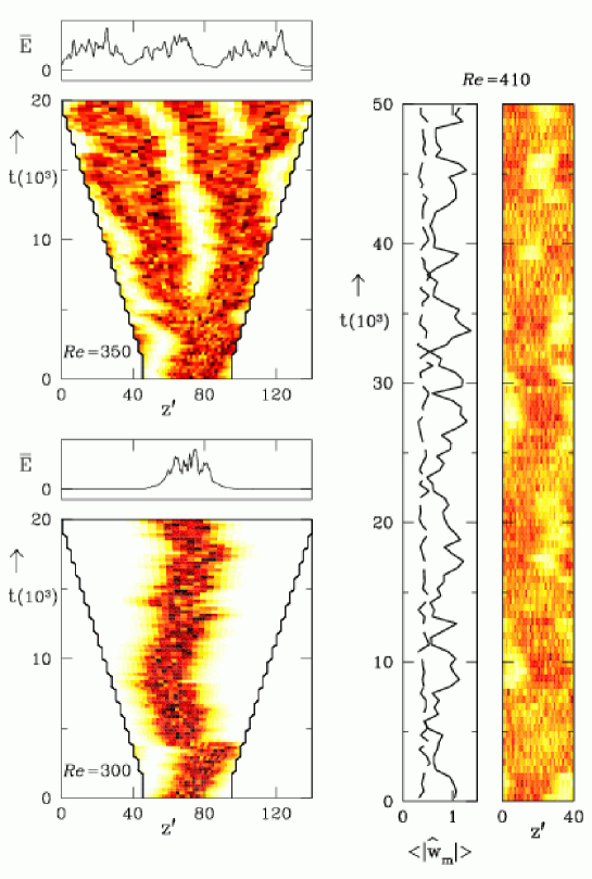
Figure 12: Simulations at $Re=350$, $Re=300$, and $Re=410$ illustrating three qualitatively different regimes. For the simulations at $Re=350$ and $Re=300$, $L_{z^{\prime}}$ is increased from 50 to 140. The state at $Re=350$ is periodic: the turbulent band divides as $L_{z^{\prime}}$ is increased to retain a wavelength near 40. The final kinetic energy profile $\bar{E}({z^{\prime}})$ is bounded away from zero. The state at $Re=300$ is localized: a single turbulent band persists, regardless of domain size and $\bar{E}({z^{\prime}})$ decays exponentially to zero away from the band. The simulation at $Re=410$ is carried out at $L_{z^{\prime}}=40$. The state is intermittent: laminar regions appear and disappear and the average spectral coefficients corresponding to $m=1$ (solid) and $m=0$ (dashed) oscillate erratically.

The turbulent-laminar patterned states shown in Figure 11 are of three qualitatively different types Barkley and Tuckerman (2005). We demonstrate this by carrying out three long simulations, at three different Reynolds numbers, that are shown in Figure 12. In this figure, the energy along the line ${x^{\prime}}=y=0$ for the 32 points in ${z^{\prime}}$ has been averaged over windows of length $T=500$ to yield a value shown by the shading of each space-time rectangle.

The simulations at $Re=350$ and $Re=300$ are carried out by increasing the long direction of our domain, $L_{z^{\prime}}$, in regular discrete increments of 5 from $L_{z^{\prime}}=50$ to $L_{z^{\prime}}=140$. At $Re=350$, a single turbulent band is seen when $L_{z^{\prime}}=50$. This band divides into two when $L_{z^{\prime}}=65$ and a third band appears when $L_{z^{\prime}}=130$: the periodic pattern adjusts to keep the wavelength in the range 35–65. This is close to the wavelength range observed experimentally by Prigent et al., which is 46–60. When the same protocol is followed at $Re=300$, no additional turbulent bands appear as $L_{z^{\prime}}$ is increased. We call the state at $Re=300$ localized and note that turbulent spots are reported near these values of $Re$ in the experiments. The small $L_{x^{\prime}}$ of our computational domain does not permit localization in the ${x^{\prime}}$ direction; instead localized states must necessarily take the form of bands when visualized in the $x$-$z$ plane.

The instantaneous integrated kinetic energy profile

$$\bar{E}\equiv\int\,d{x^{\prime}}\,dy\>E({x^{\prime}},y,{z^{\prime}})$$

is plotted at the final time for both cases. For $Re=350$, $\bar{E}$ does not reach zero and the flow does not revert to the simple Couette solution between the turbulent bands, as could also be seen in the earlier visualizations (Figures 7, 9). In contrast, for $Re=300$, $\bar{E}$ decays to zero exponentially, showing that the flow approaches the simple Couette solution away from the turbulent band. In this case, there is truly coexistence between laminar and turbulent flow regions.

The simulation at $Re=410$ illustrates another type of behavior. In a domain of length $L_{z^{\prime}}=40$, laminar or, rather, weakly-fluctuating regions appear and disappear. The spectral coefficients corresponding to $m=1$ (wavelength 40) and $m=0$ oscillate erratically. Similar states at similar Reynolds numbers are reported experimentally by Prigent and coworkers (2001,2002,2003,2005), where they are interpreted as resulting from noise-driven competition between banded patterns at equal and opposite angles, a feature necessarily absent from our simulations.

V DEPENDENCE ON ANGLE

V.1 Angle survey

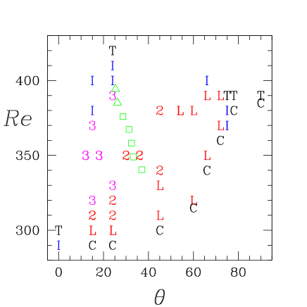
Figure 13: Patterns as a function of Reynolds number $Re$ and $\theta$, the angle between the $L_{x^{\prime}}$ direction of our rectangular computational domain and the streamwise direction. The domain is of size $L_{x^{\prime}}\times L_{y}\times L_{z^{\prime}}=(4/\sin\theta)\times 2\times 120$. For each angle, upper and lower limits in $Re$ are shown for each regime. T: uniform turbulence (lower limit in $Re$). I: intermittent turbulence. 3: pattern containing three turbulent-laminar bands, each of approximate wavelength 40. 2: pattern containing two bands of approximate wavelength 60. L: pattern containing one turbulent region, possibly localized. C: laminar Couette flow (no patterns observed below this $Re$). Open symbols show experimental observations of Prigent et al.  Triangles: patterns with wavelength between 46 and 50. Squares: patterns with wavelength between 50 and 60.

We have explored the angles with respect to the streamwise direction at which a turbulent-laminar pattern may exist. The results are plotted in Figure 13. We keep $L_{z\prime}=120$ and $L_{x^{\prime}}=4/\sin\theta$. The transition from uniform turbulence to laminar Couette flow occurs via intermediate states which occupy a decreasing range of $Re$ as $\theta$ is increased. The sequence of states seen for increasing $\theta$ at $Re=350$ is qualitatively the same as that for decreasing $Re$ at $\theta=24^{\circ}$: uniform turbulence at $\theta=0^{\circ}$, a turbulent-laminar pattern with three bands at $\theta=15^{\circ}$ to $\theta=24^{\circ}$, two bands for $\theta=30^{\circ}$ and $\theta=45^{\circ}$, a localized state for $\theta=66^{\circ}$, and laminar Couette flow for $\theta^{\circ}\geq 72$. Thus far we have obtained patterns for angles between $15^{\circ}$ and $66^{\circ}$ and the number of bands decreases with angle.

Experimental data from Prigent and coworkers (2001,2003,2005) is also shown in Figure 13. The wavelengths, angles, and Reynolds numbers reported ranged from $\lambda_{z^{\prime}}=46.3$ and $\theta=25.3^{\circ}$ at $Re=394$ to $\lambda_{z^{\prime}}=60.5$ and $\theta=37^{\circ}$ at $Re=340$. In these ranges of angle and Reynolds number, we observe a similar trend, since our wavelength (constrained here to be a divisor of $L_{z^{\prime}}=120$) increases from 40 to 60 as the number of bands decreases from 3 to 2. Between $Re=325$ and $Re=280$, experiments showed spots, which may correspond to some of the states we have labeled as localized in Figure 13. At present, we do not systematically distinguished localized states from others containing one turbulent region but which may not behave like Figure 12. The threshold for intermittency is also difficult to define and to determine.

The most striking difference between our computations and the experimental data is that the range of angles over which we find periodic turbulent-laminar patterns (from $\theta=15^{\circ}$ to at least $\theta=45^{\circ}$) is far greater than that seen in the experiment. Patterns with angles outside of the experimental range are likely to be unstable in a large domain in which the angle is unconstrained.

Our computational technique requires that the size of the domain be increased as $\theta$ decreases according to $L_{x^{\prime}}=4/\sin\theta$ in order to respect the spanwise vortex or streak spacing; see Figure 3. Hence the computational cost increases with decreasing $\theta$ and for this reason we have not as yet investigated $\theta$ between $15^{\circ}$ and $0^{\circ}$. For $\theta$ exactly $0^{\circ}$, this trigonometric constraint is lifted, since the streamwise vortices and streaks would not extend diagonally across the rectangular domain, but parallel to its boundaries. As $\theta$ increases, the domain size $L_{x^{\prime}}=4/\sin\theta$ decreases, as does the computation cost. For $\theta$ between $45^{\circ}$ and $90^{\circ}$, for which $L_{x^{\prime}}$ is between 5.7 and 4, we reduce the number of spectral elements in the ${x^{\prime}}$ direction from 10 to 4 (see Figure 4).

Figure 14: Evolution for $\theta=90^{\circ}$. Two simulations at $Re=400$ are shown, in domains with $L_{x^{\prime}}=L_{z}=4$. The domain shown on the right has $L_{z^{\prime}}=L_{x}=220$; that on the left has $L_{z^{\prime}}=L_{x}=6$, close to the minimal flow unit (the two are not shown to scale). The large domain supports a transient pattern as an intermediate state between uniform turbulence and laminar Couette flow, whereas the turbulence persists in the small domain.

V.2 Long streamwise direction

For $\theta=90^{\circ}$, the domain has a long streamwise direction $L_{z^{\prime}}=L_{x}$ and a short spanwise direction $L_{x^{\prime}}=L_{z}$. Figure 13 shows that, for $\theta=90^{\circ}$ and $L_{x}=120$, we obtain direct decay from uniform turbulence to laminar Couette flow at $Re=385$. We have varied $L_{x}$ and show the results in Figure 14. When $L_{x}=220$, the turbulence is extinguished at $Re=400$; a transient pattern of wavelength 110 can be seen. But when $L_{x}=6$, we find that the turbulence persists down to a value of $Re\approx 370$. We recall that the minimal flow unit was proposed by Hamilton et al. (1995) as the smallest which can support the streak and streamwise-vortex cycle and maintain turbulence; the flow becomes laminar when either of the dimensions are reduced below their MFU values. However, Figure 14 shows that turbulence can also sometimes be extinguished by increasing $L_{x}$. Simulations in domains with a long streamwise and a short spanwise dimension have also been carried out by Jiménez et al. Jiménez et al. (2005) with the goal of understanding the role of the streamwise dimension, e.g. streak length.

Figure 15: Evolution for $\theta=0^{\circ}$ with $L_{x^{\prime}}=L_{x}=10$ and $L_{z^{\prime}}=L_{z}=120$. $Re$ is lowered by steps of $\Delta Re=5$; not all intermediate values of $Re$ are shown. The flow continues to have turbulent regions far below $Re=300$. Left: evolution over the entire domain, showing the formation and disappearance of turbulent domains. Right: evolution of $w(x=0,y=0,z=60,t)$, showing irregular periodic cycles.

V.3 Long spanwise direction

In the case $\theta=0^{\circ}$, the domain has a long spanwise direction ($L_{z}=L_{z^{\prime}}=120$) and a short streamwise direction ($L_{x}=L_{x^{\prime}}=10$). In decreasing the Reynolds number by $\Delta Re=5$ after each interval of $T=1000$, we observe turbulent regions far below $Re=300$, terminating only at $Re=210$, as shown in Figure 15. At several times, the turbulence seems ready to disappear, only to spread out again. In order to confirm this surprising result, we have carried out longer simulations at each of these low values of $Re$. Turbulence persisted over $T=4200$ (in the usual advective time units) at $Re=220$, over $T=3000$ at $Re=225$, and even over $T=15000$ for $Re=230$.

Experiments Dauchot and Daviaud (1995) and numerical simulations in large domains ($L_{x}\times L_{y}\times L_{z}=128\times 2\times 64$) Lundbladh and Johansson (1991) and numerical simulations in periodic minimal flow units ($L_{x}\times L_{y}\times L_{z}=4\times 2\times 6$) Hamilton et al. (1995) have produced long-lived turbulence only for $Re>300$. A number of studies Schmiegel and Eckhardt (1997, 2000); Faisst and Eckhardt (2004); Eckhardt and Faisst (2005) have examined turbulent lifetimes as a function of initial perturbation amplitude, Reynolds number, and quenching rate (rate of Reynolds number decrease) in minimal flow units. In these studies, turbulence with a lifetime greater than $T=2000$ was counted as sustained; experiments Dauchot and Daviaud (1995), however, are carried out on timescales several orders of magnitude longer than this. Schmiegel and Eckhardt (2000) studied the effect of quenching rate on turbulent lifetimes. For rates of Reynolds number decrease comparable to ours, they found that turbulence could in some cases subsist to $Re=280$ or 290 for times on the order of $T=1000$ to 10000; for quenching rates ten times faster than ours, turbulence was occasionally sustained to $Re=240$.

If we compare our results to the previous simulations, then the conclusion would be that turbulence is favored by a short streamwise direction $L_{x}=10$ and a long spanwise direction $L_{z}=120$. When either of these two conditions are lifted, the turbulence disappears. We note, however, that our simulations do not systematically vary the initial conditions and thus do not determine the probability of long-lived turbulence at these low Reynolds numbers near $220$.

We also note that Toh and colleagues Toh and Itano (2005); Toh et al. (2005) have recently reported results from simulations of Couette flow in domains with long spanwise extent compared with the MFU geometry. These simulations are for higher values of $Re$ than those considered here.

We observe an approximately periodic oscillation in time, shown on the right of Figure 15. The oscillation period of about 200 time units has the same order of magnitude as the minimum turbulent cycle Hamilton et al. (1995), but further analysis of our results is required before we can identify the streak and streamwise-vortex cycle in our flow.

VI SUMMARY

We have used an extension of the minimal-flow-unit methodology to study large-scale turbulent-laminar patterns formed in plane Couette flow. Turbulent-laminar patterns are obtained as solutions to the Navier–Stokes equations in domains with a single long direction. The other dimensions are just large enough to resolve the inter-plate distance and to contain an integer number of longitudinal vortex pairs or streaks. We have presented various visualizations of the computed turbulent-laminar patterns as well as space-time plots illustrating the formation and dynamics of these patterns. The time-averaged modulus of the spatial Fourier spectrum is shown to provide a quantitative diagnosis of the patterns. Periodic, localized, and intermittent states occur in our simulations where similar states are observed experimentally.

We have explored the patterns’ dependence on Reynolds number, domain length and tilt angle. The patterned states do not appear to depend sensitively on how the turbulence is initialized nor on the route taken to a particular point in parameter space. It is, however, possible that some parameter combinations may support different numbers of turbulent bands (although we have not yet observed this). All states are bistable with respect to laminar Couette flow and if parameters are changed too abruptly, then reversion to laminar Couette flow occurs.

It appears that large-scale patterns are inevitable intermediate states on the route from turbulent to laminar flow in large aspect-ratio Couette flow. A key open question is what mechanism causes laminar-turbulent patterns. These patterns are not only interesting in and of themselves, but may provide clues to the transition to turbulence in plane Couette flow.

References

- Barkley and Tuckerman (1999) Barkley, D. and Tuckerman, L.S. (1999). Stability analysis of perturbed plane Couette flow. Phys. Fluids 11, 1187–1195.
- Barkley and Tuckerman (2005) Barkley, D. and Tuckerman, L.S. (2005). Computational study of turbulent laminar patterns in Couette flow. Phys. Rev. Lett. 94, 014502.
- Bottin et al. (1998) Bottin, S., Dauchot, O., Daviaud, F. and Manneville, P. (1998). Experimental evidence of streamwise vortices as finite amplitude solutions in transitional plane Couette flow. Phys. Fluids 10, 2597–2607.
- Coles (1965) Coles, D. (1965). Transition in circular Couette flow. J. Fluid Mech. 21, 385–425.
- Coles and van Atta (1966) Coles, D. and van Atta, C.W. (1966). Progress report on a digital experiment in spiral turbulence. AIAA J. 4, 1969–1971.
- Cros and Le Gal (2002) Cros, A. and Le Gal, P. (2002). Spatiotemporal intermittency in the torsional Couette flow between a rotating and a stationary disk. Phys. Fluids 14, 3755–3765.
- Dauchot and Daviaud (1995) Dauchot, O. and Daviaud, F. (1995). Finite-amplitude perturbation and spots growth-mechanism in plane Couette flow. Phys. Fluids 7, 335–343.
- Eckhardt and Faisst (2005) Eckhardt, B. and Faisst, H. (2005). Dynamical systems and the transition to turbulence. In Proceedings of the IUTAM Symposium on Non-Uniqueness of Solutions to the Navier–Stokes Equations and Their Connection with Laminar-Turbulent Transition, T. Mullin and R. Kerswell (eds), Springer, Dordrecht, pp. 35–50.
- Faisst and Eckhardt (2004) Faisst, H. and Eckhardt, B. (2004). Sensitive dependence on initial conditions in transition to turbulence in pipe flow. J. Fluid Mech. 504, 343–352.
- Hamilton et al. (1995) Hamilton, J.M., Kim, J. and Waleffe, F. (1995). Regeneration mechanisms of near-wall turbulence structures. J. Fluid Mech. 287, 317–348.
- Hegseth (1996) Hegseth, J.J. (1996). Turbulent spots in plane Couette flow. Phys. Rev. E 54, 4915–4923.
- Henderson and Karniadakis (1995) Henderson, R.D. and Karniadakis, G.E. (1995). Unstructured spectral element methods for simulation of turbulent flows. J. Comput. Phys. 122, 191–217.
- Hof et al. (2003) Hof, B., Juel, A. and Mullin, T. (2003). Scaling of the turbulence transition threshold in a pipe. Phys. Rev. Lett. 91, 244502.
- Jiménez et al. (2005) Jiménez, J., Kawahara, G., Simens, M.P. and del Alamo, J.C. (2005). The near-wall structures of turbulent wall flows. In Proceedings of the IUTAM Conference on Elementary Vortices and Coherent Structures, S. Kida (ed.), Springer, Dordrecht.
- Jiménez and Moin (1991) Jiménez, J. and Moin, P. (1991). The minimal flow unit in near-wall turbulence. J. Fluid Mech. 225, 213–240.
- Lundbladh and Johansson (1991) Lundbladh, A. and Johansson, A.V. (1991). Direct simulation of turbulent spots in plane Couette flow. J. Fluid Mech. 229, 499–516.
- Prigent (2001) Prigent, A. (2001). La spirale turbulente: Motif de grande longueur d’onde dans les écoulements cisallés turbulents. PhD Thesis, University Paris-Sud.
- Prigent et al. (2002) Prigent, A., Grégoire, G., Chaté, H., Dauchot, O. and van Saarloos, W. (2002). Large-scale finite-wavelength modulation within turbulent shear flows. Phys. Rev. Lett. 89, 014501.
- Prigent et al. (2003) Prigent, A., Grégoire, G., Chaté, H. and Dauchot, O. (2003). Long-wavelength modulation of turbulent shear flows. Physica D 174, 100–113.
- Prigent and Dauchot (2005) Prigent, A. and Dauchot, O. (2005). Transition versus front turbulence in subcritical Couette flows. In Proceedings of the IUTAM Symposium on Non-Uniqueness of Solutions to the Navier–Stokes Equations and Their Connection with Laminar-Turbulent Transition, T. Mullin and R. Kerswell (eds), Springer, Dordrecht, pp. 193–217.
- Schmiegel and Eckhardt (1997) Schmiegel, A. and Eckhardt, B. (1997). Fractal stability border in plane Couette flow. Phys. Rev. Lett. 79, 5250–5253.
- Schmiegel and Eckhardt (2000) Schmiegel, A. and Eckhardt, B. (2000). Persistent turbulence in annealed plane Couette flow. Europhys. Lett. 51, 395–400.
- Toh and Itano (2005) Toh, S. and Itano, T. (2005). Interaction between a large-scale structure and near-wall structure in channel flow. J. Fluid Mech. 524, 249–262.
- Toh et al. (2005) Toh, S., Itano, T. and Satoh, K. (2005). Co-supporting cycle: Sustaining mechanism of large-scale structures and near-wall structures in channel flow turbulence. In Proceedings of the IUTAM Symposium on Non-Uniqueness of Solutions to the Navier–Stokes Equations and Their Connection with Laminar-Turbulent Transition, T. Mullin and R. Kerswell (eds), Springer, Dordrecht, pp. 71–83.
- Tuckerman and Barkley (2002) Tuckerman, L.S. and Barkley, D. (2002). Symmetry breaking and turbulence in perturbed plane Couette flow. Theoret. Comput. Fluid Dynam. 16, 43–48.
- van Atta (1966) van Atta, C.W. (1966). Exploratory measurements in spiral turbulence. J. Fluid Mech. 25, 495–512.
- Waleffe (2003) Waleffe, F. (2003). Homotopy of exact coherent structures in plane shear flows. Phys. Fluids 15, 1517–1534.
- Waleffe (2005) Waleffe, F. and Wang, J.(2005). In Proceedings of the IUTAM Symposium on Non-Uniqueness of Solutions to the Navier–Stokes Equations and Their Connection with Laminar-Turbulent Transition, T. Mullin and R. Kerswell (eds), Springer, Dordrecht, pp. 85–106.